LOFAR observations of fine spectral structure dynamics in type IIIb radio bursts

1 Introduction

During solar flares beams of accelerated electrons propagating along the open magnetic field lines can produce the so-called type III radio bursts (Benz, 2008; Holman et al., 2011). They are observed as fast drifting structures in radio dynamic spectra with high brightness temperature (see Suzuki and Dulk, 1985; Pick and Vilmer, 2008; Benz, 2008, as recent reviews). The type III radio bursts can be traced from the solar corona into the interplanetary space (e.g. Lin, 1974; Klassen, Gómez-Herrero, and Heber, 2011; Krupar et al., 2014; Alissandrakis et al., 2015), where the corresponding electron beams and the beam-driven Langmuir waves near the electron plasma frequency $f_{\mathrm{pe}}$ can be observed in-situ (Lin, 1985; Krucker et al., 2007). In the dynamic spectra of type III bursts,the fundamental ($\approx f_{\mathrm{pe}}$) and harmonic ($\approx 2f_{\mathrm{pe}}$) parallel drifting components are usually identified (McLean and Labrum, 1985).

A large fraction of metric and decametric type III radio bursts reveal fine spectral structuring. In particular, the so-called type IIIb radio bursts (de La Noe and Boischot, 1972; Abranin et al., 1979; Mugundhan, Hariharan, and Ramesh, 2017) are characterized by multiple narrowband bursts with slow frequency drift, known as stria bursts. They compose the fast drifting spectral structure similar to usual type III radio bursts (Ellis and McCulloch, 1967; Ellis, 1969; de La Noe and Boischot, 1972; Stewart, 1975; Takakura and Yousef, 1975; Baselian et al., 1974). Striae can be observed in both the fundamental and harmonic emission components, although the harmonic striae are more diffusive (Baselyan et al., 1974); if present, they can form the so called IIIb–IIIb pairs (Abranin et al., 1979; Brazhenko et al., 2015). A typical stria frequency bandwidth is of about $\sim 30-300$ kHz with the frequency drift rate of $0-150$ kHz $\textrm{s}^{-1}$ (Bhonsle, Sawant, and Degaonkar, 1979; Krüger, 1984). Duration of an individual stria depends on its frequency and is of about $\sim 1$ second for the fundamental component and can be several time longer for the harmonic emission (Bhonsle, Sawant, and Degaonkar, 1979; Krüger, 1984).

The basic explanation of striae origin is the existence of density variations along the electron beam path; this idea was firstly proposed by Takakura and Yousef (1975). Numerical modelling of Kontar (2001) demonstrated that the spatial distribution of Langmuir waves is strongly modulated by small-amplitude density fluctuations creating “Langmuir wave clumps” that could be responsible for individual striae. Estimations in that work showed that even relatively weak density perturbations ($\Delta n/n\sim 10^{-3}$, where $n$ is the thermal electron density) are sufficient to form the observed fine spectral structures. However, it is still not clear which magnetohydrodynamic (MHD) waves cause these density fluctuations; there is a long list of possible mechanisms responsible for the emission modulation (Melrose, 1982). Furthemore, until now the number of studies devoted to investigation of striae spectral properties at different frequencies was limited, while a successful theory should be able to explain both the observed striae drift rates and bandwidths as well as their frequency dependencies.

In this paper, we analyze two IIIb bursts observed with the LOw Frequency ARray (LOFAR, van Haarlem et al., 2013) on 16 April 2015. The frequency resolution of LOFAR is sufficient to resolve striae; it allows also studying the spatial characteristics of the emission sources. While the spatial dynamics of the striae sources in the mentioned event was analyzed in detail in the paper of Kontar et al. (2017), the main aim of this paper is to investigate the spectral characteristics of the striae (i.e., bandwidth and frequency drift) and their dependencies on the emission frequency. Our particular interest is to verify applicability of the density fluctuations model to explaining the observed striae properties.

2 LOFAR observations

LOw Frequency ARray (LOFAR, van Haarlem et al., 2013) was designed by the Netherlands Institute for Radio Astronomy (ASTRON). It is working in the metric-decametric wavelengths range and is able to produce spatially resolved solar observations with high time cadence and excellent spectral resolution. In this work we analyse the low-band observations (in the 30-80 MHz range) made with the LOFAR core stations located near Exloo, Netherlands; all 24 core stations (scattered over the area of $\sim 3\times 2$ $\textrm{km}^{2}$) were used for the observations.

Instead of a classical interferometric approach, the spatially-resolved spectroscopic observations were performed using the LOFAR beam-formed mode (Stappers et al., 2011; van Haarlem et al., 2013), when the data from the LOFAR core stations are combined to form a number of “tied-array beams” covering an area of the sky; the beam size is of about $\lambda/D\sim 10^{\prime}$ at 32 MHz, where $\lambda$ is the wavelength and $D$ is the maximum baseline. The advantage of using the tied-array beams is that it allows producing images with very high time resolution, which is not possible in the LOFAR interferometric mode (see Stappers et al., 2011; Morosan et al., 2014, 2015; Reid and Kontar, 2017; Chen et al., 2018, for details).

In this work the LOFAR configuration included 127 beams covering the solar disk and adjacent areas with the separation between the beam centers of about $356^{\prime\prime}$ (see Figure ims). The fluxes corresponding to each beam were recorded with high frequency and time resolution ($12.2$ kHz and 10 ms, respectively). Flux calibration was made using observations of the Crab nebula (Tau A) as it was demonstrated by Kontar et al. (2017); Chen et al. (2018). In the below light curves and dynamic spectra, the pre-event (pre-burst) background is subtracted.

3 Main properties of the selected events

3.1 LOFAR dynamic spectra of the selected type IIIb radio bursts

DSp The observations were made on 16 April 2015, around the local noon; a number of type III bursts were detected. Among them, we selected two bursts shown in Figure dyn_spec; these bursts were chosen because they are isolated, i.e., do not overlap with other bursts. The bursts occurred at $\sim$11:56:20 and $\sim$11:56:55 UT; below, they are referred to as burst 1 and burst 2, respectively. We note that there were no flares or coronal mass ejections during the considered time interval; the nearest flare (of C2 GOES class) was at $\sim$10:45:00 UT. Both bursts reveal the typical two-component (fundamental-harmonic) structure of dynamic spectra; the fine spectral structures (striae) are well visible in both of them. Below we demonstrate in detail the analysis technique and results for burst 2 (the brighter one); the other one is analyzed in the same way. The statistical results are shown for both bursts.

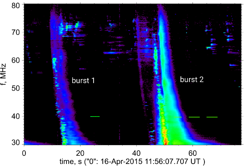
Figure 1.: Spatially-integrated background-subtracted calibrated LOFAR dynamic spectrum of two subsequent type IIIb radio bursts.dyn˙spec

In Figure zoom we show zoomed dynamic spectra of burst 2 for the chosen frequency and time ranges. These ranges are marked by rectangular boxes in top left panel of the figure. As said above, the burst is composed of two distinct components: a bright (fundamental) component with well-pronounced striae is followed by a more diffusive drifting structure (harmonic); hence the analyzed bursts can be identified as type IIIb–III pairs. The drift rates of both components are comparable and are of about 10 MHz $\textrm{s}^{-1}$ that corresponds to the electron beam speed of $\sim 0.3c$ assuming the one-fold Newkirk coronal density model (Newkirk, 1961). The dynamic spectra of the diffusive component (harmonic) reveal fine spectral structures, too (see box 3 in Figure zoom); these structures look like smoothed striae. Below, we analyze in detail the striae detected in the first bright (fundamental) component since they are more distinctive (see boxes 1 and 2 in Figure zoom).

As an example, we show in the right-bottom panel of Figure zoom the time profiles of the total (spatially-integrated) radio flux at two frequencies: $f_{1}=34.54$ MHz and $f_{2}=56.33$ MHz; the frequencies were chosen to ensure that the corresponding radio fluxes (i.e., the fundamental and harmonic components) peak at the same time. Therefore the harmonic-fundamental ratio at this particular time can be estimated as $f_{2}/f_{1}\approx 1.63$, which is relatively low but not unprecedented for type III bursts (Suzuki and Dulk, 1985).

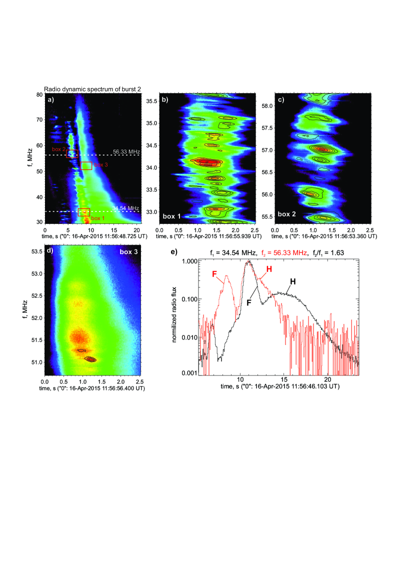
Figure 2.: a) Dynamic spectrum of burst 2; three rectangular boxes show the regions of dynamic spectrum presented in other panels. b-d) Zoomed regions of the dynamic spectrum corresponding to the fundamental (b-c) and harmonic (d) components; the contours mark striae. e) Light curves at two selected frequencies demonstrating the fundamental-harmonic relation.zoom

In panels (b-d) of Figure zoom, individual striae with high contrast are highlighted by contours; the contour levels are chosen to ensure that the contours are not too long (with the length below a threshold of 250 pixels of dynamic spectrum) and hence they, as a rule, enclose separate striae rather than groups of striae. The stria durations vary in the range of $0.5-1$ s. One can notice that the striae have frequency dependent drift rate: the stria drift rate is larger at higher frequencies; this behaviour is typical of the type III radio bursts in general. Also, the high-frequency striae have a slightly larger bandwidth than the low-frequency ones. In Section stat_spec, these frequency variations of the stria parameters are analyzed quantitatively.

3.2 Dynamics of the radio emission source

Figure ims shows two examples of the LOFAR radio images (at different times and frequencies) obtained by interpolation of the fluxes corresponding to different beams using the radial basis function method. At low frequencies, we can see a single well-defined radio emission source located on the solar disk; the signal-to-noise ratio is remarkably high. At higher frequencies (see, e.g., right panel in Figure ims), additional weaker and smaller sources appear that are likely caused by the instrument sidelobes. For these reasons, we analyze the spatial characteristics of the emission source up to the frequency of $\approx 50$ MHz only; on the other hand, the spectral characteristics of the striae are analyzed up to 70 MHz. From Figure ims, one can notice that with an increase of the emission frequency the emission source shifts eastward, and its size decreases. The raw images do not allow us to inspect dynamics of the source position with a sufficient accuracy; therefore, to describe the source parameters quantitatively and to study temporal dynamics, we fitted it by an elliptical Gaussian defined by seven free parameters: normalization coefficient, center position ($x_{0}$ and $y_{0}$), size ($\sigma_{x}$ and $\sigma_{y}$), and tilt angle. Both the parameters and their confidence limits (errors) were estimated using the least-squares procedure. Only the LOFAR beams located within $1000^{\prime\prime}$ from the solar disk center were used in the fitting procedure.

We should note that the observed radio map is a convolution of the real brightness distribution with the LOFAR beam. In a simple case when both the emission source and the LOFAR beam have approximately Gaussian shapes, the real source area $A_{\mathrm{real}}$ is determined as $A_{\mathrm{real}}\approx A_{\mathrm{obs}}-A_{\mathrm{beam}}$ where $A_{\mathrm{obs}}$ and $A_{\mathrm{beam}}$ are the areas of the observed emission source and the LOFAR beam, respectively. Thus, firstly, the apparent increase of emission source size with decreasing frequency seems to be caused mainly by the LOFAR beam broadening with decreasing frequency. Kontar et al. (2017) estimated the real source size for the considered event as $17-22$ arcmin around 32 MHz, which is approximately twice larger than the LOFAR beam at that frequency. Secondly, the expansion/shrinking rate of the emission source at a fixed frequency (which is applicable to a narrowband stria) satisfies the relation $\mathrm{d}A_{\mathrm{real}}/\mathrm{d}t=\mathrm{d}A_{\mathrm{obs}}/\mathrm{d}t$ (because the LOFAR beam size at a fixed frequency is constant). That is why the expansion rates of individual striae (considered below) are not affected by the mentioned convolution effect.

In addition, in the observed frequency range the ionospheric refraction can result in displacement of the apparent radio emission source. LOFAR monitoring of the point-like source Tau A revealed absence of significant intensity scintillations on the subsecond time scales; the level of ionospheric turbulence at the time of observations was low. To minimize the (possible) ionospheric effects, we focus on relative motions in the plane of sky at single frequency at the timescales shorter than the ionospheric scintilations observed.

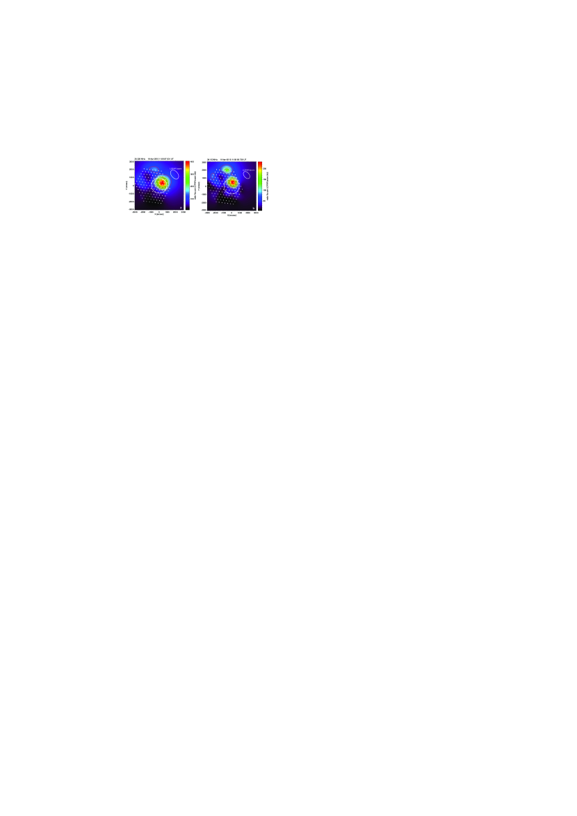
Figure 3.: LOFAR radio images at two time-frequency points within burst 2. Centers of 127 LOFAR beams are shown by small white squares. The solar limb is shown by white thick circle. The LOFAR beams sizes (at $1/2$ level) at the considered frequencies are shown by white ellipses.ims

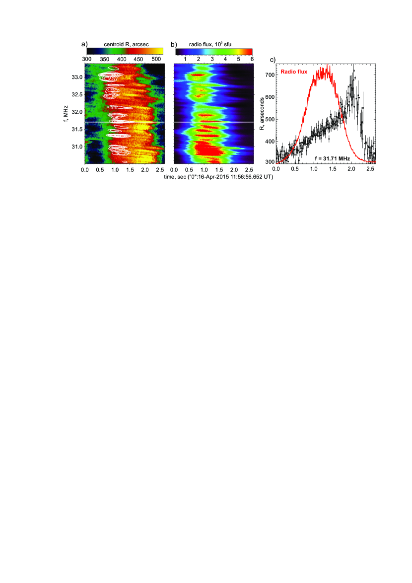
Figure 4.: Dynamics of the emission source position on the solar disk (for a sub-region of burst 2, fundamental component). a) Radial distance from the solar disk center shown by colored background as function of time and frequency; the emission intensity contours (white) are overplotted to mark striae. b) The corresponding dynamic spectrum. c) Time profile of the mentioned radial distance at a fixed frequency (31.71 MHz); the intensity lightcurve (in relative units) is overplotted.RST

Figure RST presents comparison of fine structures seen in dynamic spectra with the radial shift of the emission source position, for a region of the dynamic spectrum corresponding to the fundamental component of burst 2; the time resolution is 12.5 ms. The radial position of the source is calculated as offset of Gaussian centroid from the solar disk center; in panel a of Figure RST, the source position is shown in a dynamic-spectrum style (by colored background). Panel b presents corresponding region of the dynamic spectrum. In the panel c the dynamics of the radial distance at a chosen single frequency (31.71 MHz) is shown. The emission intensity is overplotted by white contours (in panel a) or red lightcurve (in panel c). Both the time-frequency plots (for all striae) and single-frequency time profiles demonstrate a complicated pattern reported earlier by Kontar et al. (2017): the emission source position is characterized by a gradually increasing radial distance (i.e., motion towards the limb) with a subsequent fast return motion. The evolution of the source position is delayed with respect to the intensity enhancement; the maximum radial distance is achieved $\sim 1$ s after the intensity peak, consistent with the conclusion by Kontar et al. (2017) that this behaviour most likely reflects the radio emission propagation effects.

3.3 Parameters of individual striae

case_study Figures stria1_b1–stria2_b1 present examples of individual striae. We have selected two striae within burst 1, with the frequencies around 30.11 MHz (Figure stria1_b1) and 41.77 MHz (Figure stria2_b1); below in this Section, we refer to them as to the “low-frequency” (LF) and “high-frequency” (HF) striae, respectively. To determine the stria parameters, we fitted the emission spectrum (containing several spectral channels which were selected manually for each stria burst) in each time bin by a Gaussian with a linear background. This provides us with the time-dependent values of the stria central frequency and bandwidth (determined at one-sigma level); the radio flux and emission source size and position shown in Figures stria1_b1–stria2_b1 correspond to the mentioned (variable) central frequency.

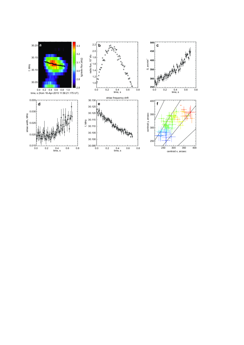
Figure 5.: An example of “low-frequency” stria. a) Dynamic spectrum. Black dots mark the central frequency of the stria (obtained by Gaussian fitting) in each time bin. b) Emission intensity (at the central frequencies) vs. time. c) Area of the radio emission source (at the central frequencies) vs. time. d) Spectral bandwidth of the stria vs. time. e) Central frequency of the stria vs. time. f) Source position on the solar disk at different times (color-coded, with the time increasing from violet to red); black lines show radial directions from the disk center.stria1˙b1

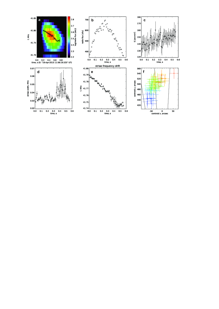
Figure 6.: Same as in Figure stria1_b1, for a “high-frequency” stria.stria2˙b1

One can see that the emission source experiences gradual expansion with time: from 270 to 450 $\textrm{arcmin}^{2}$ for the LF stria and from 135 to 155 $\textrm{arcmin}^{2}$ for the HF stria. Also, both considered striae demonstrate motion of the emission sources in a mostly radial direction, similar to the behaviour observed at a fixed frequency (see Figure RST).

The real emission source size can be estimated using the above-mentioned relation $A_{\mathrm{real}}\approx A_{\mathrm{obs}}-A_{\mathrm{beam}}$, from which we estimate the linear source size (FWHM) in the plane of sky as $l_{\mathrm{real}}\approx 2\sigma_{\mathrm{real}}\sqrt{2\ln 2}\approx(2\sqrt{2\ln 2}/\pi)\sqrt{A_{\mathrm{obs}}-A_{\mathrm{real}}}\approx 0.75\sqrt{A_{\mathrm{obs}}-A_{\mathrm{real}}}$. For the LF stria peak, considering $A_{\mathrm{real}}\approx 320$ arcmin² and $A_{\mathrm{beam}}\approx 110$ arcmin², we obtain $l_{\mathrm{real}}\approx 11$ arcmin; for the HF stria peak, we have $A_{\mathrm{real}}\approx 145$ arcmin², $A_{\mathrm{beam}}\approx 60$ arcmin², and $l_{\mathrm{real}}\approx 7$ arcmin.

Spatial extent of the source along the line-of-sight (including the effects of scattering) can be estimated from FWHM of temporal stria intensity profile in the same way as in the work of Kontar et al. (2017). For the both LF and HF striae, the duration at a fixed frequency $\Delta t$ is about 0.6 seconds; thus the upper limit of the spatial extent is $(l_{\mathrm{LOS}})_{\max}=c\Delta t\approx 180~{}\textrm{Mm}\approx 4$ arcmin. The size of the stria emission source along the line-of-sight $l_{\mathrm{LOS}}$ is smaller than the size measured across the line-of-sight; thus, studying separate striae we confirmed the conclusion of Kontar et al. (2017) that the radio wave scattering in the corona is highly anisotropic.

The LF stria bandwidth increases with time from 38 to 54 kHz, while the HF stria reveals no trend in bandwidth evolution. To estimate a characteristic (mean) stria bandwidth, we calculated a cumulative stria spectrum by summation of the spectra in all relevant time bins (shifted to provide the same central frequency). Then the bandwidth of the resulting spectrum (at one-sigma level) is considered to be a characteristic stria bandwidth; it is of about 44 kHz for the LF stria and 68 kHz for the HF stria (the HF stria is wider). Also, the HF stria reveals faster frequency drift compared with the LF stria: the drift rate can be estimated as $-27$ kHz $\textrm{s}^{-1}$ for the LF stria and $-98$ kHz $\textrm{s}^{-1}$ for the HF stria.

A similar analysis was performed for all identified striae in the bursts 1 and 2, with the results presented and summarized in the next Section.

4 Statistics of the striae parameters

4.1 Dynamics of the emission sources

stat_sourc We have selected for quantitative analysis 43 striae in burst 1 and 40 striae in burst 2. Top panels in Figure stat_source show central positions of the radio emission sources for different times and frequencies; the average positions and the characteristic (average) velocities of the emission sources for the selected striae are shown as well. To determine an average vector of the emission source velocity in the plane of the sky, we used linear fits of $x_{0}(t)$ and $y_{0}(t)$ dependencies, where $(x_{0},y_{0})$ are the central coordinates of the emission source; the corresponding average speeds (absolute magnitudes) are shown in the bottom panel (a) of Figure stat_source. A similar procedure (linear fitting) was used to determine a characteristic expansion rate of the emission source $\mathrm{d}S/\mathrm{d}t$, see bottom panel (b) of Figure stat_source. We do not show the error bars for $x_{0}$ and $y_{0}$ in top panels of Figure stat_source because this would make the figure unreadable due to the large number of data points; the typical error bars at two representative frequencies are shown in Figures stria1_b1f and stria2_b1f.

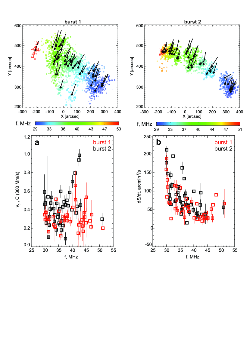
Figure 7.: Upper panels: central positions of the radio emission sources; color marks the emission frequency and black dots show the average positions of the radio emission sources for different striae. Black lines show the average velocities (direction and relative magnitude) of the striae radio emission sources. Bottom panels: speeds (a) and area expansion rates (b) of the radio emission sources for different striae vs. the striae central frequencies; red and black colors mark bursts 1 and 2, respectively.stat˙source

One can see that the obtained speeds of the striae radio emission sources $v_{\mathrm{c}}$ are mostly in the range of $(0.1-0.6)c$ and only a few points are outside this range. The area expansion rate of the emission source can be as high as $\sim 200$ $\textrm{arcmin}^{2}$ $\textrm{s}^{-1}$. Assuming that the emission source has a roughly circular shape, we can estimate the corresponding linear expansion rate as $\mathrm{d}r_{\bot}/\mathrm{d}t\approx(\mathrm{d}S/\mathrm{d}t)/(2\pi\sqrt{S})$; this value is also comparable with the speed of light and can be as high as $0.2c$. The expansion rate of the emission source tends to decrease with an increase of the emission frequency.

4.2 Statistics of the striae bandwidths and frequency drift rates

stat_spec The left panel of Figure stat_wdfdt shows the striae bandwidths calculated according to the technique described in Section case_study. The resulting data points are fitted by linear functions (separately for the bursts 1 and 2) with the equations written within the plot. The striae bandwidth increases with an increase of frequency for both bursts; typical striae widths at 30 and 60 MHz are of about 40 and 60 kHz, respectively (i.e., just a few LOFAR frequency channels). The relative bandwidth $\Delta f/f$ is weakly variable being of about 0.13% and 0.10% at the mentioned frequencies. We can conclude that the linear fits for both type IIIb bursts are similar to each other, and an average stria bandwidth increases with frequency by $\sim 0.6$ kHz per MHz.

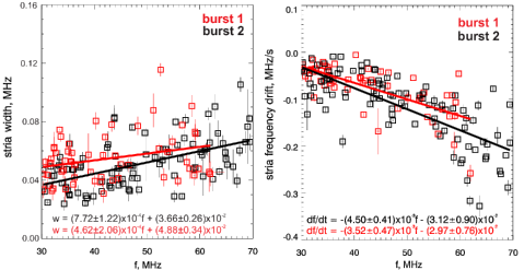
Figure 8.: Statistics of the striae bandwidths (left) and frequency drift rates (right). Solid lines represent linear fits to the data points. Red and black colors show the results for burst 1 and 2, respectively.stat˙wdfdt

The frequency drift rate of the striae increases with an increase of the emission frequency, too (see the right panel of Figure stat_wdfdt); it varies from $\sim 30$ kHz $\textrm{s}^{-1}$ at 30 MHz up to $\sim 150$ kHz $\textrm{s}^{-1}$ at 60 MHz. The obtained linear fits (stria drift rate vs. frequency) for both considered type IIIb bursts are similar to each other: $\mathrm{d}f/\mathrm{d}t\simeq 0.004f$. Note that the striae drift rates are much smaller than the typical drift rate of usual type III bursts, which normally decreases with frequency as $\mathrm{d}f/\mathrm{d}t\simeq 0.01f^{1.84}$ (Alvarez and Haddock, 1973).

5 Discussion

The most straightforward scenario for the striae formation in the type III bursts is an existence of plasma density fluctuations along the electron beam path (Takakura and Yousef, 1975). These small-amplitude density perturbations can modulate the Langmuir waves generation substantially (Kontar, 2001) and hence produce fine structures like striae in the dynamic radio spectra.

Results obtained in this work (see Section stat_spec) can be used to estimate the properties of the density irregularities that are responsible for striation. Assuming that the emission is produced at the local plasma frequency, we estimate the relative density variations corresponding to the stria bursts as $\Delta n/n\simeq 2\Delta f/f$, where $\Delta f$ is bandwidth of a stria and $f$ is its central frequency. From the linear fits in the right panel of Figure stat_wdfdt, we determined $\Delta n/n$ at different frequencies (see Figure estia) for both type IIIb bursts. The amplitude of the density fluctuations varies from $\sim 2.0\times 10^{-3}$ at 70 MHz to $\sim 3.2\times 10^{-3}$ at 30 MHz; the error bars show possible ranges of $\Delta n/n$ considering errors of linear fitting presented in Figure stat_wdfdt.

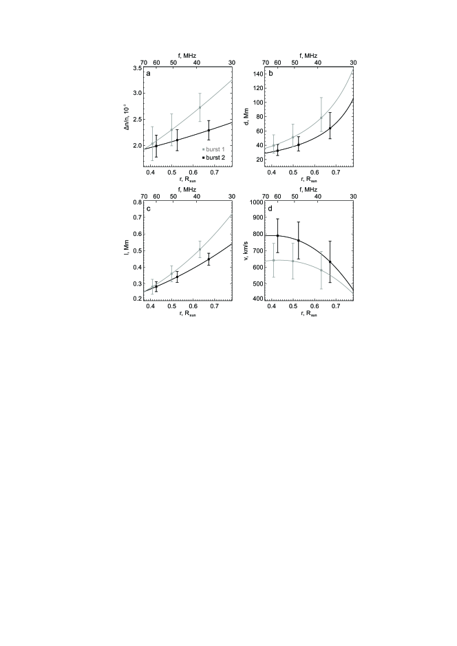
Figure 9.: Various parameters inferred from the striae bandwidths, durations, and drift rates: a) amplitude of the plasma density perturbations $\Delta n/n$; b) characteristic electron beam length $d$; c) characteristic length scale of the plasma inhomogeneities $l$; d) propagation speed of the plasma density perturbations. The respective heights are calculated according to the Newkirk coronal density model.esti

Longitudinal (i.e., along the magnetic field) size of the electron cloud generating the radio emission can be estimated as $d\sim v_{\mathrm{b}}\tau$, where $v_{\mathrm{b}}$ is the electron beam speed and $\tau$ is the characteristic time of interaction between the electron cloud and a particular density inhomogeneity. We assume that the electron beam speed is $v_{\mathrm{b}}=0.3c$ which is consistent with the estimations obtained in Section DSp; the time $\tau$ can be estimated as $\tau\sim\Delta f(\mathrm{d}f/\mathrm{d}t)^{-1}$, where $\Delta f$ is a stria bandwidth and $\mathrm{d}f/\mathrm{d}t$ is its frequency drift rate. Note that we do not consider the stria duration as $\tau$, because the stria duration can be affected by propagation effects (Kontar et al., 2017) resulting in a radio echo and extending the radio pulses; therefore the above expression characterizes the intrinsic properties of the radio emission source more accurately. The obtained values of the electron beam size vary from $\sim 20$ Mm to $\sim 150$ Mm and increase with a decrease of the stria frequency (see Figure estib). We interpret this as an expansion of the electron beam during its propagation in the solar corona, which is likely determined by geometry of open magnetic flux tube where the electrons propagate.

The characteristic length scale $l$ of the plasma inhomogeneities producing the striae bursts is related to the striae bandwidth as

$$l\approx 2n\left(\frac{\mathrm{d}n}{\mathrm{d}r}\right)^{-1}\frac{\Delta f}{f}\approx 653\left[\log_{10}\left(\frac{f}{f_{0}}\right)\right]^{-2}\frac{\Delta f}{f},$$ (1)

where $n$ is the plasma density and $r$ is the distance along the electron beam path. The second expression in the above formula was obtained by assuming radial propagation of the energetic electrons and the Newkirk coronal density model (Newkirk, 1961), with $f_{0}=1.84$ MHz and the resulting value of $l$ in Mm units. The estimated values of $l$ vary in the range of $\sim(0.2-0.8)$ Mm; they increase with a decrease of the stria frequency (see Figure estic). These inhomogeneities are much smaller than the electron beam: $l/d\sim(0.2-2.6)$%.

Similarly, the characteristic propagation speed $v_{\mathrm{p}}$ of the plasma inhomogeneities is related to the striae frequency drift rate as

$$v_{\mathrm{p}}\approx 2n\left(\frac{\mathrm{d}n}{\mathrm{d}r}\right)^{-1}\frac{1}{f}\frac{\mathrm{d}f}{\mathrm{d}t}\approx 6.53\times 10^{5}\left[\log_{10}\left(\frac{f}{f_{0}}\right)\right]^{-2}\frac{1}{f}\frac{\mathrm{d}f}{\mathrm{d}t},$$ (2)

with the resulting value of $v_{\mathrm{p}}$ in the second expression in km $\textrm{s}^{-1}$ units. The estimated values of the propagation speed vary in the range of $400-800$ $\textrm{km~{}s}^{-1}$ (see Figure estid) that corresponds to typical speeds of MHD waves (Roberts, 2000); thus, the striae frequency drift can be caused by the motion of the plasma density perturbations due to MHD waves (e.g. Kolotkov, Nakariakov, and Kontar, 2018, for details). These perturbations appear supersonic with the speeds which are $2-4$ times larger than a typical sound speed of $c_{\mathrm{s}}\approx 147\sqrt{T/[1~{}\mathrm{MK}]}\approx 200$ km $\textrm{s}^{-1}$ for a typical coronal plasma temperature of $T\approx 2$ MK (Aschwanden, 2005).

6 Conclusion

We presented detailed analysis of spatially-resolved multi-frequency LOFAR observations of two type IIIb radio bursts. The results obtained provide statistically significant properties of individual striae and hence essential constraints for the theories describing the fine spectral structure of type IIIb bursts. The main results can be summarized as follows:

• Spatial position of the radio emission sources is characterized by radial motion from the Sun centre in the sky plane. The motion is particularly well pronounced during the decay phase of a striae.

• Evolution of the spatial source position is delayed by $\sim 1$ s with respect to the radio intensity time profiles.

• The apparent speed of the radio emission sources in the plane of sky is $(0.1-0.6)c$; the expansion speed of the sources is up to $\sim 0.2c$.

• Instantaneous bandwidth of the striae increases with an increase of the central frequency; the bandwidths lie in the range of $20-100$ kHz that corresponds to the relative bandwidth $\Delta f/f$ of about $0.06-0.12$%.

• Frequency drift rate of the striae increases with an increase of the central frequency; the drift rates lie in the range of $0-0.3$ MHz $\textrm{s}^{-1}$.

• The relative amplitudes of the plasma density fluctuations that may be responsible for the formation of the striae should be of about $(2-3)\times 10^{-3}$.

• The characteristic sizes and propagation speeds of the mentioned density fluctuations are expected to be of about $200-800$ km and $400-800$ km $\textrm{s}^{-1}$, respectively. The propagation speeds are substantially larger than the typical sound speed of 200 km $\textrm{s}^{-1}$ in the corona and closer to the typical Alfvén speed (Régnier, Priest, and Hood, 2008).

• Estimations of the apparent radio source size (with account for the scattering effects) indicate that the source size across the line-of-sight exceeds considerably the size along the line-of-sight; this implies that scattering of the radio waves must be anisotropic.

The results obtained from analysis of two type IIIb bursts with striae support the conclusion of Kontar et al. (2017) that the sizes of the radio emission sources and their dynamics are determined by the radio wave propagation effects. At the same time, dynamics of the source motions does not support a simple scenario of an isotropic radio source and isotropic radio wave scattering (e.g., Steinberg et al., 1971; Arzner and Magun, 1999); reproducing the observed source dynamics and diagnosing the scattering regime require more complicated scattering simulations. The narrowband “striae” bursts are produced, most likely, by small-scale small-amplitude plasma density perturbations in the solar corona connected with propagating MHD waves. These MHD perturbations propagate with the speed larger than the sound speed and closer to Alfvén (fast magnetoacoustic) speed in the corona.

Acknowledgments

The work has benefited from a Marie Curie International Research Staff Exchange Scheme “Radiosun” (PEOPLE-2011-IRSES-295272), an international team grant (http://www.issibern.ch/teams/lofar/) from ISSI Bern, Switzerland, the Program No. 28 of the RAS Presidium, and budgetary funding of Basic Research program II.16. E.P.K. was supported by Science and Technology Facilities Council Grant (STFC) No. ST/P000533/1. This paper is based (in part) on data obtained from facilities of the International LOFAR Telescope (ILT) under project code LC3-012. LOFAR (van Haarlem et al., 2013) is the Low Frequency Array designed and constructed by ASTRON. It has observing, data processing, and data storage facilities in several countries, that are owned by various parties (each with their own funding sources), and that are collectively operated by the ILT foundation under a joint scientific policy. The ILT resources have benefitted from the following recent major funding sources: CNRS-INSU, Observatoire de Paris and Université d’Orléans, France; BMBF, MIWF-NRW, MPG, Germany; Science Foundation Ireland (SFI), Department of Business, Enterprise and Innovation (DBEI), Ireland; NWO, The Netherlands; The Science and Technology Facilities Council, UK.

References

- Abranin et al. (1979) Abranin, E.P., Baselian, L.L., Goncharov, N.I., Zinichev, V.A., Rapoport, V.O., Tsybko, I.G.: 1979, Harmonic structure of type IIIb and III bursts. Sol. Phys. 62, 145. DOI. ADS.
- Alissandrakis et al. (2015) Alissandrakis, C.E., Nindos, A., Patsourakos, S., Kontogeorgos, A., Tsitsipis, P.: 2015, A tiny event producing an interplanetary type III burst. A&A 582, A52. DOI. ADS.
- Alvarez and Haddock (1973) Alvarez, H., Haddock, F.T.: 1973, Solar Wind Density Model from km-Wave Type III Bursts. Sol. Phys. 29, 197. DOI. ADS.
- Arzner and Magun (1999) Arzner, K., Magun, A.: 1999, Radiowave propagation in a statistically inhomogeneous plasma. A&A 351, 1165. ADS.
- Aschwanden (2005) Aschwanden, M.J.: 2005, Physics of the Solar Corona. An Introduction with Problems and Solutions (2nd edition). ADS.
- Baselian et al. (1974) Baselian, L.L., Goncharov, N.I., Zaitsev, V.V., Zinichev, V.A., Rapoport, V.O., Tsybko, I.G.: 1974, Frequency and time splitting of decameter solar radio bursts. I - Elementary events. Sol. Phys. 39, 213. DOI. ADS.
- Baselyan et al. (1974) Baselyan, L.L., Goncharov, N.Y., Zaitsev, V.V., Zinichev, V.A., Rapoport, V.O., Tsybko, Y.G.: 1974, Frequency and Time Splitting of Decameter Solar Radio Bursts. II: Chains. Sol. Phys. 39, 223. DOI. ADS.
- Benz (2008) Benz, A.O.: 2008, Flare Observations. Living Reviews in Solar Physics 5, 1. DOI. ADS.
- Bhonsle, Sawant, and Degaonkar (1979) Bhonsle, R.V., Sawant, H.S., Degaonkar, S.S.: 1979, Exploration of the solar corona by high resolution solar decametric observations. Space Sci. Rev. 24, 259. DOI. ADS.
- Brazhenko et al. (2015) Brazhenko, A.I., Melnik, V.N., Frantsuzenko, A.V., Dorovskyy, V.V., Rucker, H.O., Panchenko, M.: 2015, On the Harmonic Coupling of Components in Pairs of IIIb-III Bursts at Decameter Wavelengths. Russian Radio Physics and Radio Astronomy 20, 99. DOI. ADS.
- Chen et al. (2018) Chen, X., Kontar, E.P., Yu, S., Yan, Y., Huang, J., Tan, B.: 2018, Fine Structures of Solar Radio Type III Bursts and Their Possible Relationship with Coronal Density Turbulence. ApJ 856, 73. DOI. ADS.
- de La Noe and Boischot (1972) de La Noe, J., Boischot, A.: 1972, The type iii b burst. A&A 20, 55. ADS.
- Ellis (1969) Ellis, G.R.A.: 1969, Fine structure in the spectra of solar radio bursts. Australian Journal of Physics 22, 177. DOI. ADS.
- Ellis and McCulloch (1967) Ellis, G.R.A., McCulloch, P.M.: 1967, Frequency splitting of solar radio bursts. Australian Journal of Physics 20, 583. ADS.
- Holman et al. (2011) Holman, G.D., Aschwanden, M.J., Aurass, H., Battaglia, M., Grigis, P.C., Kontar, E.P., Liu, W., Saint-Hilaire, P., Zharkova, V.V.: 2011, Implications of x-ray observations for electron acceleration and propagation in solar flares. Space Sci. Rev. 159, 107. DOI. ADS.
- Klassen, Gómez-Herrero, and Heber (2011) Klassen, A., Gómez-Herrero, R., Heber, B.: 2011, Electron Spikes, Type III Radio Bursts and EUV Jets on 22 February 2010. Sol. Phys. 273, 413. DOI. ADS.
- Kolotkov, Nakariakov, and Kontar (2018) Kolotkov, D.Y., Nakariakov, V.M., Kontar, E.P.: 2018, The origin of the modulation of the radio emission from the solar corona by a fast magnetoacoustic wave. ArXiv e-prints. ADS.
- Kontar (2001) Kontar, E.P.: 2001, Dynamics of electron beams in the solar corona plasma with density fluctuations. A&A 375, 629. DOI. ADS.
- Kontar et al. (2017) Kontar, E.P., Yu, S., Kuznetsov, A.A., Emslie, A.G., Alcock, B., Jeffrey, N.L.S., Melnik, V.N., Bian, N.H., Subramanian, P.: 2017, Imaging spectroscopy of solar radio burst fine structures. Nature Communications 8, 1515. DOI. ADS.
- Krucker et al. (2007) Krucker, S., Kontar, E.P., Christe, S., Lin, R.P.: 2007, Solar flare electron spectra at the sun and near the earth. ApJ 663, L109. DOI. ADS.
- Krüger (1984) Krüger, A.: 1984, Introduction to solar radio astronomy and radio physics. ADS.
- Krupar et al. (2014) Krupar, V., Maksimovic, M., Santolik, O., Kontar, E.P., Cecconi, B., Hoang, S., Kruparova, O., Soucek, J., Reid, H., Zaslavsky, A.: 2014, Statistical Survey of Type III Radio Bursts at Long Wavelengths Observed by the Solar TErrestrial RElations Observatory (STEREO)/ Waves Instruments: Radio Flux Density Variations with Frequency. Sol. Phys. 289, 3121. DOI. ADS.
- Lin (1974) Lin, R.P.: 1974, Non-relativistic Solar Electrons. Space Sci. Rev. 16, 189. DOI. ADS.
- Lin (1985) Lin, R.P.: 1985, Energetic solar electrons in the interplanetary medium. Sol. Phys. 100, 537. DOI. ADS.
- McLean and Labrum (1985) McLean, D.J., Labrum, N.R.: 1985, Solar radiophysics: Studies of emission from the sun at metre wavelengths. ADS.
- Melrose (1982) Melrose, D.B.: 1982, Fine structures in Decametric noise storms : possible mechanisms. In: Benz, A.O., Zlobec, P. (eds.) Solar Radio Storms, CESRA Workshop #4, 182. ADS.
- Morosan et al. (2014) Morosan, D.E., Gallagher, P.T., Zucca, P., Fallows, R., Carley, E.P., Mann, G., Bisi, M.M., Kerdraon, A., Konovalenko, A.A., MacKinnon, A.L., Rucker, H.O., Thidé, B., Magdalenić, J., Vocks, C., Reid, H., Anderson, J., Asgekar, A., Avruch, I.M., Bentum, M.J., Bernardi, G., Best, P., Bonafede, A., Bregman, J., Breitling, F., Broderick, J., Brüggen, M., Butcher, H.R., Ciardi, B., Conway, J.E., de Gasperin, F., de Geus, E., Deller, A., Duscha, S., Eislöffel, J., Engels, D., Falcke, H., Ferrari, C., Frieswijk, W., Garrett, M.A., Grießmeier, J., Gunst, A.W., Hassall, T.E., Hessels, J.W.T., Hoeft, M., Hörandel, J., Horneffer, A., Iacobelli, M., Juette, E., Karastergiou, A., Kondratiev, V.I., Kramer, M., Kuniyoshi, M., Kuper, G., Maat, P., Markoff, S., McKean, J.P., Mulcahy, D.D., Munk, H., Nelles, A., Norden, M.J., Orru, E., Paas, H., Pandey-Pommier, M., Pandey, V.N., Pietka, G., Pizzo, R., Polatidis, A.G., Reich, W., Röttgering, H., Scaife, A.M.M., Schwarz, D., Serylak, M., Smirnov, O., Stappers, B.W., Stewart, A., Tagger, M., Tang, Y., Tasse, C., Thoudam, S., Toribio, C., Vermeulen, R., van Weeren, R.J., Wucknitz, O., Yatawatta, S., Zarka, P.: 2014, LOFAR tied-array imaging of Type III solar radio bursts. A&A 568, A67. DOI. ADS.
- Morosan et al. (2015) Morosan, D.E., Gallagher, P.T., Zucca, P., O’Flannagain, A., Fallows, R., Reid, H., Magdalenić, J., Mann, G., Bisi, M.M., Kerdraon, A., Konovalenko, A.A., MacKinnon, A.L., Rucker, H.O., Thidé, B., Vocks, C., Alexov, A., Anderson, J., Asgekar, A., Avruch, I.M., Bentum, M.J., Bernardi, G., Bonafede, A., Breitling, F., Broderick, J.W., Brouw, W.N., Butcher, H.R., Ciardi, B., de Geus, E., Eislöffel, J., Falcke, H., Frieswijk, W., Garrett, M.A., Grießmeier, J., Gunst, A.W., Hessels, J.W.T., Hoeft, M., Karastergiou, A., Kondratiev, V.I., Kuper, G., van Leeuwen, J., McKay-Bukowski, D., McKean, J.P., Munk, H., Orru, E., Paas, H., Pizzo, R., Polatidis, A.G., Scaife, A.M.M., Sluman, J., Tasse, C., Toribio, M.C., Vermeulen, R., Zarka, P.: 2015, LOFAR tied-array imaging and spectroscopy of solar S bursts. A&A 580, A65. DOI. ADS.
- Mugundhan, Hariharan, and Ramesh (2017) Mugundhan, V., Hariharan, K., Ramesh, R.: 2017, Solar Type IIIb Radio Bursts as Tracers for Electron Density Fluctuations in the Corona. Sol. Phys. 292, 155. DOI. ADS.
- Newkirk (1961) Newkirk, G. Jr.: 1961, The Solar Corona in Active Regions and the Thermal Origin of the Slowly Varying Component of Solar Radio Radiation. ApJ 133, 983. DOI. ADS.
- Pick and Vilmer (2008) Pick, M., Vilmer, N.: 2008, Sixty-five years of solar radioastronomy: flares, coronal mass ejections and sun earth connection. A&A Rev. 16, 1. DOI. ADS.
- Régnier, Priest, and Hood (2008) Régnier, S., Priest, E.R., Hood, A.W.: 2008, Coronal Alfvén speeds in an isothermal atmosphere. I. Global properties. A&A 491, 297. DOI. ADS.
- Reid and Kontar (2017) Reid, H.A.S., Kontar, E.P.: 2017, Imaging spectroscopy of type U and J solar radio bursts with LOFAR. A&A 606, A141. DOI. ADS.
- Roberts (2000) Roberts, B.: 2000, Waves and Oscillations in the Corona - (Invited Review). Sol. Phys. 193, 139. DOI. ADS.
- Stappers et al. (2011) Stappers, B.W., Hessels, J.W.T., Alexov, A., Anderson, K., Coenen, T., Hassall, T., Karastergiou, A., Kondratiev, V.I., Kramer, M., van Leeuwen, J., Mol, J.D., Noutsos, A., Romein, J.W., Weltevrede, P., Fender, R., Wijers, R.A.M.J., Bähren, L., Bell, M.E., Broderick, J., Daw, E.J., Dhillon, V.S., Eislöffel, J., Falcke, H., Griessmeier, J., Law, C., Markoff, S., Miller-Jones, J.C.A., Scheers, B., Spreeuw, H., Swinbank, J., Ter Veen, S., Wise, M.W., Wucknitz, O., Zarka, P., Anderson, J., Asgekar, A., Avruch, I.M., Beck, R., Bennema, P., Bentum, M.J., Best, P., Bregman, J., Brentjens, M., van de Brink, R.H., Broekema, P.C., Brouw, W.N., Brüggen, M., de Bruyn, A.G., Butcher, H.R., Ciardi, B., Conway, J., Dettmar, R.-J., van Duin, A., van Enst, J., Garrett, M., Gerbers, M., Grit, T., Gunst, A., van Haarlem, M.P., Hamaker, J.P., Heald, G., Hoeft, M., Holties, H., Horneffer, A., Koopmans, L.V.E., Kuper, G., Loose, M., Maat, P., McKay-Bukowski, D., McKean, J.P., Miley, G., Morganti, R., Nijboer, R., Noordam, J.E., Norden, M., Olofsson, H., Pandey-Pommier, M., Polatidis, A., Reich, W., Röttgering, H., Schoenmakers, A., Sluman, J., Smirnov, O., Steinmetz, M., Sterks, C.G.M., Tagger, M., Tang, Y., Vermeulen, R., Vermaas, N., Vogt, C., de Vos, M., Wijnholds, S.J., Yatawatta, S., Zensus, A.: 2011, Observing pulsars and fast transients with LOFAR. A&A 530, A80. DOI. ADS.
- Steinberg et al. (1971) Steinberg, J.L., Aubier-Giraud, M., Leblanc, Y., Boischot, A.: 1971, Coronal Scattering, Absorption and Refraction of Solar Radiobursts. A&A 10, 362. ADS.
- Stewart (1975) Stewart, R.T.: 1975, An example of a fundamental type IIIb radio burst. Sol. Phys. 40, 417. DOI. ADS.
- Suzuki and Dulk (1985) Suzuki, S., Dulk, G.A.: 1985, In: McLean, D.J., Labrum, N.R. (eds.) Bursts of Type III and Type V, Cambridge University Press, Cambridge and New York, 289. ADS.
- Takakura and Yousef (1975) Takakura, T., Yousef, S.: 1975, Type IIIb radio bursts - 80 MHz source position and theoretical model. Sol. Phys. 40, 421. DOI. ADS.
- van Haarlem et al. (2013) van Haarlem, M.P., Wise, M.W., Gunst, A.W., Heald, G., McKean, J.P., Hessels, J.W.T., de Bruyn, A.G., Nijboer, R., Swinbank, J., Fallows, R., Brentjens, M., Nelles, A., Beck, R., Falcke, H., Fender, R., Hörandel, J., Koopmans, L.V.E., Mann, G., Miley, G., Röttgering, H., Stappers, B.W., Wijers, R.A.M.J., Zaroubi, S., van den Akker, M., Alexov, A., Anderson, J., Anderson, K., van Ardenne, A., Arts, M., Asgekar, A., Avruch, I.M., Batejat, F., Bähren, L., Bell, M.E., Bell, M.R., van Bemmel, I., Bennema, P., Bentum, M.J., Bernardi, G., Best, P., Bîrzan, L., Bonafede, A., Boonstra, A.-J., Braun, R., Bregman, J., Breitling, F., van de Brink, R.H., Broderick, J., Broekema, P.C., Brouw, W.N., Brüggen, M., Butcher, H.R., van Cappellen, W., Ciardi, B., Coenen, T., Conway, J., Coolen, A., Corstanje, A., Damstra, S., Davies, O., Deller, A.T., Dettmar, R.-J., van Diepen, G., Dijkstra, K., Donker, P., Doorduin, A., Dromer, J., Drost, M., van Duin, A., Eislöffel, J., van Enst, J., Ferrari, C., Frieswijk, W., Gankema, H., Garrett, M.A., de Gasperin, F., Gerbers, M., de Geus, E., Grießmeier, J.-M., Grit, T., Gruppen, P., Hamaker, J.P., Hassall, T., Hoeft, M., Holties, H.A., Horneffer, A., van der Horst, A., van Houwelingen, A., Huijgen, A., Iacobelli, M., Intema, H., Jackson, N., Jelic, V., de Jong, A., Juette, E., Kant, D., Karastergiou, A., Koers, A., Kollen, H., Kondratiev, V.I., Kooistra, E., Koopman, Y., Koster, A., Kuniyoshi, M., Kramer, M., Kuper, G., Lambropoulos, P., Law, C., van Leeuwen, J., Lemaitre, J., Loose, M., Maat, P., Macario, G., Markoff, S., Masters, J., McFadden, R.A., McKay-Bukowski, D., Meijering, H., Meulman, H., Mevius, M., Middelberg, E., Millenaar, R., Miller-Jones, J.C.A., Mohan, R.N., Mol, J.D., Morawietz, J., Morganti, R., Mulcahy, D.D., Mulder, E., Munk, H., Nieuwenhuis, L., van Nieuwpoort, R., Noordam, J.E., Norden, M., Noutsos, A., Offringa, A.R., Olofsson, H., Omar, A., Orrú, E., Overeem, R., Paas, H., Pandey-Pommier, M., Pandey, V.N., Pizzo, R., Polatidis, A., Rafferty, D., Rawlings, S., Reich, W., de Reijer, J.-P., Reitsma, J., Renting, G.A., Riemers, P., Rol, E., Romein, J.W., Roosjen, J., Ruiter, M., Scaife, A., van der Schaaf, K., Scheers, B., Schellart, P., Schoenmakers, A., Schoonderbeek, G., Serylak, M., Shulevski, A., Sluman, J., Smirnov, O., Sobey, C., Spreeuw, H., Steinmetz, M., Sterks, C.G.M., Stiepel, H.-J., Stuurwold, K., Tagger, M., Tang, Y., Tasse, C., Thomas, I., Thoudam, S., Toribio, M.C., van der Tol, B., Usov, O., van Veelen, M., van der Veen, A.-J., ter Veen, S., Verbiest, J.P.W., Vermeulen, R., Vermaas, N., Vocks, C., Vogt, C., de Vos, M., van der Wal, E., van Weeren, R., Weggemans, H., Weltevrede, P., White, S., Wijnholds, S.J., Wilhelmsson, T., Wucknitz, O., Yatawatta, S., Zarka, P., Zensus, A., van Zwieten, J.: 2013, LOFAR: The LOw-Frequency ARray. A&A 556, A2. DOI. ADS.