IMPULSIVELY GENERATED WAVE TRAINS IN CORONAL STRUCTURES: II. EFFECTS OF TRANSVERSE STRUCTURING ON SAUSAGE WAVES IN PRESSURELESS SLABS

Abstract

Impulsively generated sausage wave trains in coronal structures are important for interpreting a substantial number of observations of quasi-periodic signals with quasi-periods of order seconds. We have previously shown that the Morlet spectra of these wave trains in coronal tubes depend crucially on the dispersive properties of trapped sausage waves, the existence of cutoff axial wavenumbers and the monotonicity of the dependence of the axial group speed on the axial wavenumber in particular. This study examines the difference a slab geometry may introduce, for which purpose we conduct a comprehensive eigenmode analysis, both analytically and numerically, on trapped sausage modes in coronal slabs with a considerable number of density profiles. For the profile descriptions examined, coronal slabs can trap sausage waves with longer axial wavelengths, and the group speed approaches the internal Alfvén speed more rapidly at large wavenumbers in the cylindrical case. However, common to both geometries, cutoff wavenumbers exist only when the density profile falls sufficiently rapidly at distances far from coronal structures. Likewise, the monotonicity of the group speed curves depends critically on the profile steepness right at the structure axis. Furthermore, the Morlet spectra of the wave trains are shaped by the group speed curves for coronal slabs and tubes alike. Consequently, we conclude that these spectra have the potential for telling the sub-resolution density structuring inside coronal structures, although their detection requires an instrumental cadence of better than $\sim 1$ second.

1 INTRODUCTION

Magnetohydrodynamic (MHD) waves and oscillations abound in the highly structured solar atmosphere (see e.g., Nakariakov & Verwichte 2005; Banerjee et al. 2007; De Moortel & Nakariakov 2012; Wang 2016; Nakariakov et al. 2016, for recent reviews). On the one hand, these waves may play an important role in atmospheric heating (see e.g., Klimchuk 2006; Parnell & De Moortel 2012; Arregui 2015; De Moortel & Browning 2015, for some recent reviews). On the other hand, when placed in the framework of MHD wave theory, the measurements of these waves and oscillations can help yield the atmospheric parameters that prove difficult to measure directly. This practice was originally proposed for coronal applications (e.g., Uchida 1970; Rosenberg 1970; Zajtsev & Stepanov 1975) and hence termed coronal seismology (Roberts et al. 1984; also see the reviews by, e.g., Roberts 2000, Roberts 2008). With the advent of advanced space-borne and ground-based instruments, MHD waves and oscillations have also been identified in jet-like structures such as spicules (e.g., De Pontieu et al. 2007, He et al. 2009, and the review by Zaqarashvili & Erdélyi 2009) and network jets (Tian et al. 2014), prominences (e.g., Arregui et al. 2012, and references therein), pores and sunspots (e.g., Dorotovič et al. 2008; Morton et al. 2011; Dorotovič et al. 2014; Grant et al. 2015; Freij et al. 2016), as well as various chromospheric structures (e.g., Jess et al. 2009; Morton et al. 2012). For this reason, the seismological practice is now commonly referred to as solar magneto-seismology (SMS). Furthermore, while traditionally applied to the inference of the physical parameters of localized structures, the ideas behind SMS have also been extended to the so-called “global coronal seismology” (Warmuth & Mann 2005; Ballai 2007), which capitalizes on the measurements of various large-scale waves to deduce the global magnetic field in the corona (see e.g., Liu & Ofman 2014; Warmuth 2015; Chen 2016, for recent reviews).

We restrict ourselves to the applications of SMS to the solar corona. Perhaps the magnetic field strength in coronal loops tops the list of the physical parameters that one would like SMS to offer. This is understandable because the magnetic field is known to play an essential role in shaping the corona but is notoriously difficult to directly measure (e.g., Cargill 2009). Indeed, standing kink modes have largely been exploited for this purpose since they were first imaged by the Transition Region and Coronal Explorer (TRACE, Aschwanden et al. 1999 and Nakariakov et al. 1999) and subsequently by Hinode (Ofman & Wang 2008; Erdélyi & Taroyan 2008), the Solar TErrestrial RElations Observatories (STEREO, Verwichte et al. 2009 ) and the Solar Dynamics Observatory/Atmospheric Imaging Assembly (SDO/AIA, e.g., Aschwanden & Schrijver 2011; White & Verwichte 2012). It is just that the longitudinal Alfvén time ($L/v_{\rm Ai}$ with $L$ being the loop length and $v_{\rm Ai}$ being the Alfvén speed at the loop axis) rather than the magnetic field strength itself is the direct outcome of the measured kink mode periods. However, inferring the information on density structuring transverse to coronal structures can be as important, because this structuring significantly affects the heating efficiencies of such wave-based mechanisms as phase-mixing (Heyvaerts & Priest 1983) and resonant absorption (e.g., Hollweg & Yang 1988; Ruderman & Roberts 2002; Goossens et al. 2002). To proceed, let $\rho_{\rm i}$ ($\rho_{\rm e}$) denote the density at the loop axis (in the ambient corona), $R$ denote the loop radius, and $l$ denote the transverse density length scale. If one attributes the damping of standing kink modes to resonant absorption, then their periods and damping rates can be combined to constrain $L/v_{\rm Ai}$ and the transverse density structuring as characterized by $\rho_{\rm i}/\rho_{\rm e}$ and $l/R$ (e.g., Arregui et al. 2007a; Goossens et al. 2008; Soler et al. 2014; Arregui & Asensio Ramos 2014).

Standing sausage modes in magnetized loops can also be exploited for inferring both the magnetic field strength and the transverse density structuring. To see this, consider the simplest case where the gas pressure is negligible and coronal structures are seen as straight, field-aligned cylinders with physical parameters transversely distributed in a top-hat manner. Furthermore, focus for now on the lowest-order modes. It is well-known that trapped modes arise when the axial wavenumber $k$ exceeds some cutoff value $k_{\rm c}$, and leaky modes arise when the opposite is true (e.g., Edwin & Roberts 1983; Cally 1986; Kopylova et al. 2007; Nakariakov et al. 2012; Chen et al. 2015a, 2016). It turns out that the period $P\approx 2.6R/v_{\rm Ai}$ and the damping-time-to-period ratio $\tau/P\approx(\rho_{\rm i}/\rho_{\rm e})/\pi^{2}$ for standing sausage modes in sufficiently long loops (e.g., Kopylova et al. 2007). This means that one can readily derive the transverse Alfvén time $R/v_{\rm Ai}$ from the measured periods and the density contrast $\rho_{\rm i}/\rho_{\rm e}$ from the measured damping-time-to-period ratios, provided that lateral leakage is the mechanism for the apparent wave damping. Things become more complicated if one considers that the transverse density distribution is more likely to be continuous. In this case, $P$ and $\tau/P$ turn out to depend on the transverse density length scale as well. This then enables one to constrain the combination $[R/v_{\rm Ai},\rho_{\rm i}/\rho_{\rm e},l/R]$, as illustrated in Chen et al. (2015b) where we adopted the widely accepted idea that a substantial fraction of quasi-periodic pulsations (QPPs) in solar flare emissions are attributable to standing sausage modes in flare loops (e.g., Nakariakov & Melnikov 2009; Van Doorsselaere et al. 2016). Let us note that the dimensionless transverse density length scale $l/R$ is the most difficult to constrain, an issue also associated with applications of standing kink modes in active region loops (e.g. Arregui et al. 2007a; Soler et al. 2014). However, we showed in Guo et al. (2016) that the parameter set $[R/v_{\rm Ai},\rho_{\rm i}/\rho_{\rm e},l/R]$ can be constrained to rather narrow ranges by using the measurements of co-existing standing kink and sausage modes in a flare loop that occurred on 14 May 2013 as imaged with the Nobeyama Radio Heliograph (NoRH, Kolotkov et al. 2015). The reason is simply that in this case we have more knowns than when only either a kink or sausage mode is measured.

Seismological applications can also be made of fast sausage wave trains in coronal structures. Theoretically predicted by Roberts et al. (1983) (see also Roberts et al. 1984 and Oliver et al. 2015) and numerically examined by a series of studies (e.g., Murawski & Roberts 1993, 1994; Selwa et al. 2004; Nakariakov et al. 2004; Shestov et al. 2015; Yu et al. 2016a), such modes can occur as the response of coronal structures to impulsive, internal, localized drivers such as flaring activities. When measured along the structure axis at a distance sufficiently far from the driver, the generated signals consist of three distinct phases. A nearly monochromatic “periodic phase” appears first, then a “quasi-periodic phase” arises where the signals are expected to be stronger with quasi-periods decreasing with time, and finally a monochromatic “decay or Airy phase” occurs. For coronal tubes with top-hat transverse density profiles as examined in Roberts et al. (1983) and Roberts et al. (1984), the quasi-periods in the first phase are also approximately $2.6R/v_{\rm Ai}$. On the one hand, this makes it no surprise that the candidates for impulsively generated sausage wave trains are mostly identified in high-cadence measurements in, say, optical passbands with ground-based instruments at total eclipses (e.g. Pasachoff & Landman 1984; Pasachoff & Ladd 1987; Williams et al. 2001, 2002; Katsiyannis et al. 2003; Samanta et al. 2016). On the other hand, the measured quasi-periods can then offer an estimate of the transverse Alfvén time $R/v_{\rm Ai}$ (e.g, Fu et al. 1990; Roberts 2008).

Something particularly noteworthy in the measurements of candidate sausage wave trains is the identification of tadpole-shaped Morlet spectra characterized by narrow tails preceding broad heads (e.g., Williams et al. 2001; Katsiyannis et al. 2003; Mészárosová et al. 2009; Samanta et al. 2016). The appearance of these “crazy tadpoles” largely relies on two aspects of the dependence on the axial wavenumber of the group speeds of trapped sausage modes (see Yu et al. 2017, hereafter paper I). One is the existence of cutoff wavenumbers, which guarantees that the lowest-order modes are primarily excited provided that the impulsive driver is not too localized (see also Oliver et al. 2015; Shestov et al. 2015). The other is that with $k$ increasing from the cutoff values, the group speed $v_{\rm gr}$ typically first decreases rapidly from the external Alfvén speed $v_{\rm Ae}$ to some local minimum $v_{\rm gr}^{\rm min}$ before increasing towards $v_{\rm Ai}$. The wave packets pertinent to the portion of the $v_{\rm gr}-k$ curves with $v_{\rm Ai}<v_{\rm gr}<v_{\rm Ae}$ account for the narrow tails in the “crazy tadpoles”, because the corresponding frequencies vary little. On the other hand, wave packets in the portion embedding $v_{\rm gr}^{\rm min}$ can have the same group speeds but different frequencies, meaning that they can arrive simultaneously at the point where the measurements are made. The superposition of multiple wavepackets makes the signals stronger, thereby accounting for the broad heads in the “crazy tadpoles”. However, these two features of the group speed curves are mostly found for coronal tubes with top-hat profiles. As shown by Lopin & Nagorny (2015b) and paper I, cutoff wavenumbers may not exist if the density profile far from the tubes does not fall off sufficiently rapidly with distance. Furthermore, both Yu et al. (2016a) and paper I indicated that the group speed curves can behave in a monotonical manner for coronal tubes with diffuse boundaries. It then follows that overall four different types of group speed curves arise, depending on the existence of cutoff wavenumbers and whether the curves behave in a monotonical fashion. Paper I demonstrated that the temporal evolution of impulsively generated wave trains in general, their Morlet spectra in particular, can be quite different for qualitatively different group speed curves. For instance, in the absence of wavenumber cutoffs, higher-order modes can be readily excited, resulting in the “fins” sitting atop the main bodies of the pertinent Morlet spectra. On the other hand, when the group speed curves are monotonical, the main bodies may look like obliquely directed carps rather than tadpoles. Given that the behavior of the group speed curves is determined by the transverse density distribution, paper I went on to suggest that this largely unknown distribution can be deduced by digging into the available data to look for those Morlet spectra that look drastically different from “crazy tadpoles”.

The present study is intended to continue our paper I by examining impulsively generated sausage waves in coronal slabs. The reason for doing this is threefold. First, in certain circumstances, a slab geometry is more appropriate for describing the measured waves in the solar atmosphere (e.g., Verwichte et al. 2005; Chen et al. 2010, 2011). In particular, impulsively generated sausage waves in a slab geometry have been invoked to account for a substantial number of radio emission features such as decimetric fiber bursts (e.g. Mészárosová et al. 2009, 2011; Karlický et al. 2013) and zebra-pattern structures in type IV radio bursts (Yu et al. 2016b). Second, sausage waves in a slab geometry are easier to handle mathematically. We will capitalize on this mathematical simplicity to offer a rather extensive analytical eigenmode analysis. The obtained results, together with the numerical computations, will enable us to quantify the difference a slab geometry introduces to the dispersive properties of trapped sausage waves. Third, we will explicitly show that whether the group speed curves are monotonical is almost entirely determined by the steepness of the density profile at the structure axis, which was implicated but not articulated in paper I.

This manuscript is organized as follows. Section 2 starts with a description of the equilibrium configuration, and then presents the governing equations together with their solution methods. Our methodology for studying impulsively generated wave trains is illustrated in Section 3 where the much-studied top-hat profiles are examined. A comparison for this simplest situation between the slab and cylindrical geometries shows that the results are qualitatively the same. This then inspired us to present in Section 4 our philosophy on how to examine the quantitative differences. Sections 5 to 7 then examine three families of density profiles in substantial detail. A combination of parameters that characterize sausage modes will be quantitatively compared with what we found in the cylindrical case. Finally, Sect. 8 closes this manuscript with our summary and some concluding remarks. To corroborate the results on the general behavior of the group speed curves found in the main text, we will offer a number of appendices to examine some additional density profiles that permit analytical treatments.

2 GENERAL DESCRIPTION OF METHODS FOR EXAMINING IMPULSIVELY GENERATED SAUSAGE WAVES

2.1 Description of the Equilibrium Slab

From the outset, let us restrict ourselves to typical coronal applications by working in the framework of cold MHD, in which case slow modes are absent. Adopting a Cartesian coordinate system $(x,y,z)$, we assume that the equilibrium magnetic field ${\bf B}$ is uniform and directed in the $z$-direction (${\bf B}=B\hat{z}$). To model a structured corona, we further assume that the equilibrium density $\rho$ is a function of $x$ only and symmetric about $x=0$. In the half-plane $x\geq 0$, it takes the form

$${\rho}(x)=\rho_{\rm e}+(\rho_{\rm i}-\rho_{\rm e})f(x),$$ (1)

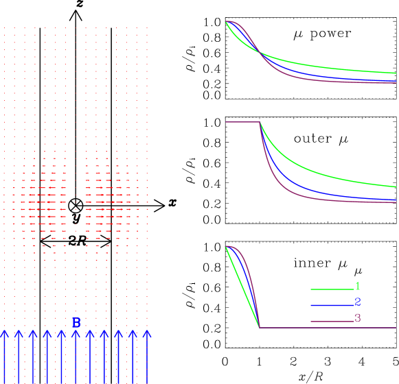
Figure 1: Description of the modeled structured corona. In the left column, in addition to an illustration of the coronal slabs, the initial perturbation to the transverse velocity is also shown by the red arrows (see Equation 15). Shown in the right column are the three families of transverse density profiles examined in this study. For illustration purposes, the density contrast $\rho_{\rm i}/\rho_{\rm e}$ is chosen to be $5$, while a number of different steepness parameters ($\mu$) are chosen as labeled.

where the function $f(x)$ decreases from unity at $x=0$ to zero when $x$ approaches infinity. Let $R$ be the spatial scale that characterizes the variation of $f(x)$. Equation (1) then mimics a density-enhanced slab with half-width $R$ embedded in an ambient corona, with the density at the slab axis being $\rho_{\rm i}$ and that far from the slab being $\rho_{\rm e}$. The Alfvén speed is given by $v_{\rm A}(x)=B/\sqrt{4\pi\rho(x)}$, which increases from $v_{\rm Ai}$ to $v_{\rm Ae}$ with $v_{\rm Ai,e}=B/\sqrt{4\pi\rho_{\rm i,e}}$. Evidently, $v_{\rm Ae}^{2}/v_{\rm Ai}^{2}=\rho_{\rm i}/\rho_{\rm e}$. The equilibrium configuration is illustrated in the left column of Fig. 1.

Following Paper I, we will focus on three families of profiles. The first one is called “$\mu$ power” and described by

$$f(x)=\displaystyle\frac{1}{1+\left(x/R\right)^{\mu}}~{}.$$ (2)

The next one, called “outer $\mu$”, is given by

$$f(x)=\left\{\begin{array}[]{ll}1,&0\leq x\leq R,\\ \left(x/R\right)^{-\mu},&x\geq R.\end{array}\right.$$ (3)

The third one is called “inner $\mu$” and in the form

$$f(x)=\left\{\begin{array}[]{ll}1-\left(\displaystyle\frac{x}{R}\right)^{\mu},&0\leq x\leq R,\\ 0,&x\geq R.\end{array}\right.$$ (4)

These profiles are illustrated in the right column of Fig. 1 where $\rho_{\rm i}/\rho_{\rm e}$ is arbitrarily chosen to be $5$. Evidently, $\mu$ is a measure of the profile steepness, and all profiles converge to a top-hat one when $\mu\rightarrow\infty$. We will consider only the cases $\mu\geq 1$, because otherwise the “$\mu$ power” and “inner $\mu$” profiles will become cusped around $x=0$. With typical EUV active region loops in mind, we will consider density contrasts in the range between $2$ and $10$ (e.g., Aschwanden et al. 2004). Note that this range is also typical of polar plumes (Wilhelm et al. 2011, Table 3). In fact, the results from this study apply to both magnetically open and closed structures.

All the profile prescriptions in Equations (2) to (4) have the following characteristics,

$$f(x)\approx\left\{\begin{array}[]{ll}1-\displaystyle\left(\frac{x}{R}\right)^{\mu_{0}},&0<x/R\ll 1,\\ \displaystyle\left(\frac{x}{R}\right)^{-\mu_{\infty}},&x/R\gg 1.\end{array}\right.$$ (7)

These characteristics, together with the specific values of $\mu_{0}$ and $\mu_{\infty}$, are summarized in the first four columns in Table 1. Evidently, with the exception of the “$\mu$ power” profile, the approximate sign in Equation (7) is actually exact. These three families of profile prescriptions are representative in the sense that one can distinguish between the steepness at the slab axis (characterized by $\mu_{0}$) and that at infinity ($\mu_{\infty}$). However, obviously they do not exhaust all possible ways for prescribing the transverse density distribution.

2.2 Governing Equations and Methods of Solution

To examine how the modeled equilibrium responds to small-amplitude initial disturbances, let $\delta\rho,\delta\mathbf{v}$ and $\delta\mathbf{b}$ represent the density, velocity, and magnetic field perturbations, respectively. Neglecting propagation out of the $x-z$ plane ($\partial/\partial y\equiv 0$) and focusing on compressible perturbations, one finds from linearized cold MHD equations that only $\delta\rho$, $\delta v_{x}$, $\delta b_{x}$ and $\delta b_{z}$ survive. A single equation can be readily derived for $\delta v_{x}(x,z;t)$, namely

$$\frac{\partial^{2}\delta v_{x}}{\partial t^{2}}=v_{\rm A}^{2}(x)\left(\displaystyle\frac{\partial^{2}}{\partial z^{2}}+\displaystyle\frac{\partial^{2}}{\partial x^{2}}\right)\delta v_{x}~{}.$$ (8)

The density perturbation $\delta\rho$ is governed by

$$\frac{\partial\delta\rho}{\partial t}=-\left(\delta v_{x}\frac{\partial\rho}{\partial x}+\rho\frac{\partial\delta v_{x}}{\partial x}\right)~{}.$$ (9)

For each profile with a given combination of $[\rho_{\rm i}/\rho_{\rm e},\mu]$, we will always start with an eigenmode analysis to establish the dispersive behavior of trapped sausage modes. Fourier-decomposing any perturbation $\delta g(x,z;t)$ as

$$\delta g(x,z;t)={\rm Re}\left\{\tilde{g}(x)\exp\left[-i\left(\omega t-kz\right)\right]\right\}~{},$$ (10)

one finds from Equation (8) that

$$\frac{{\rm d}^{2}\tilde{\xi}}{{\rm d}x^{2}}+\left(\frac{\omega^{2}}{v^{2}_{\rm A}}-k^{2}\right)\tilde{\xi}=0~{},$$ (11)

where $\tilde{\xi}=i\tilde{v}_{x}/\omega$ is the Fourier amplitude of the transverse Lagrangian displacement. With trapped sausage modes in mind, Equation (11) constitutes a standard eigenvalue problem (EVP) when supplemented with the following boundary conditions (BCs)

$$\tilde{\xi}(x=0)=0~{},\hskip 5.69046pt\tilde{\xi}(x\to\infty)\to 0~{}.$$ (12)

To solve this EVP, we employ a MATLAB boundary-value-problem solver BVPSuite in its eigen-value mode (see Kitzhofer et al. 2009 for a description of the code, and see Li et al. 2014 for an extensive validation study). What comes out is that the dimensionless angular frequency $\omega R/v_{\rm Ai}$ can be formally expressed as

$$\displaystyle\frac{\omega R}{v_{\rm Ai}}={\cal G}\left[kR;\frac{\rho_{\rm i}}{\rho_{\rm e}},f\left(\frac{x}{R}\right)\right].$$ (13)

Note that both $\omega$ and the axial wavenumber $k$ are real-valued. The axial phase and group speeds simply follow from the definitions $v_{\rm ph}=\omega/k$ and $v_{\rm gr}={\rm d}\omega/{\rm d}k$, respectively.

The dispersive properties of trapped sausage modes will provide the context for interpreting the numerical results that examine how coronal slabs respond to a localized initial perturbation. Instead of directly solving the time-dependent linear cold MHD equations, we choose to solve the equivalent version, Equation (8), which is simpler to handle. To this end, we discretize Equation (8) in a finite-difference (FD) manner on a computational domain extending from $0$ to $L_{x}$ ($-L_{z}/2$ to $L_{z}/2$) in the $x$-($z$-) direction. For simplicity, a uniform grid spacing with $\Delta z=0.08R$ is adopted in the $z$-direction. However, to speed up our computations, the grid points in the $x$-direction are chosen to be nonuniformly distributed. Let $\Delta x_{j}$ denote the spacing at grid index $j$ ($j=1,2,3,\cdots$). The spacing is fixed at $\Delta x_{1}=0.02R$ when $x\leq 3R$. We then allow $\Delta x_{j}$ to increase as $\Delta x_{j+1}=1.025\Delta x_{j}$ until it reaches $\sqrt{\rho_{\rm i}/\rho_{\rm e}}\Delta x_{1}$. From there on $\Delta x_{j}$ remains a constant again. Despite this complication, we ensure that the FD approximations to the spatial derivatives in Equation (8) are second order accurate in both the $x$- and $z$- directions. We adopt the leap-frog method for time integration, for which a uniform time step $\Delta t=0.6\Delta_{\rm min}/v_{\rm A,max}$ is chosen to comply with the Courant condition. Here $\Delta_{\rm min}$ ($v_{\rm A,max}$) represents the smallest (largest) value that the grid spacing (Alfvén speed) attains in the entire computational domain.

The boundary and initial conditions are specified as follows. At the left boundary $x=0$, we fix $\delta v_{x}$ at zero. We choose both $L_{x}$ and $L_{z}$ to be sufficiently large such that the perturbations reflected off the pertinent boundaries will not contaminate the numerical results to be analyzed. While in this regard the boundary conditions therein are irrelevant, we nonetheless fix $\delta v_{x}$ at zero in practice. To initiate our simulations, we choose to perturb only the transverse velocity, meaning that

$$\frac{\partial\delta v_{x}}{\partial t}(x,z;t=0)=0~{},$$ (14)

given the absence of $\delta b_{x}$ and $\delta b_{z}$ at $t=0$. Finally, $\delta v_{x}$ at $t=0$ is specified as

$$\displaystyle\frac{\delta v_{x}(x,z;t=0)}{v_{\rm Ai}}={\rm e}^{1/2}\left(\frac{x}{\sigma_{x}}\right)\exp\left(-\frac{x^{2}}{2\sigma_{x}^{2}}\right)\exp\left(-\frac{z^{2}}{2\sigma_{z}^{2}}\right),$$ (15)

which ensures the parity of the generated wave trains by not displacing the slab axis. Here a constant $\exp(1/2)$ is introduced such that the right hand side (RHS) of Equation (15) attains a maximum of unity. Furthermore, $\sigma_{x}$ ($\sigma_{z}$) determines the extent to which the initial perturbation spans in the transverse (axial) direction. Throughout this study, both $\sigma_{x}$ and $\sigma_{z}$ are chosen to be $R/\sqrt{2}$ such that the initial perturbation is neither too localized nor too extended. This perturbation is shown by the red arrows in the left column of Fig. 1.

Several points need to be made. First, the temporal signal we actually analyze with a wavelet analysis is the density variation $\delta\rho$. To find this, Equation (9) is advanced simultaneously with Equation (8) by assuming that $\delta\rho(x,z;t=0)=0$. Second, for each profile choice we will examine the dispersive properties of trapped sausage modes by solving the EVP (Equations 11 and 12) with BVPSuite. An analytical dispersion relation (DR) will be derived when mathematically tractable. The BVPSuite results are found to agree exactly with the numerical solutions to the pertinent DRs without exception, a point that we will not mention later. We will also derive the expressions for the cutoff wavenumbers as well as the behavior of the group speeds $v_{\rm gr}$ at large axial wavenumbers. The latter is necessary because the asymptotic behavior of $v_{\rm gr}$ largely determines whether the $v_{\rm gr}-k$ curves are monotonical. Third, it turns out that the eigenmode analysis always results in an infinite number of branches of solutions. We use the transverse harmonic number $l$ ($l=1,2,3,\cdots$) to label a branch, following the convention that $l=1$ refers to the fundamental transverse mode and $l\geq 2$ refers to its transverse harmonics.

3 CORONAL SLABS WITH TOP-HAT PROFILES

Let us start with the simplest case where the transverse density profiles are piece-wise constant. The reason for doing this exercise is to illustrate our methodology for examining impulsively generated wave trains. While the group speed behavior was traditionally invoked to interpret the temporal evolution (e.g., Murawski & Roberts 1993, 1994) and Morlet spectra (e.g., Nakariakov et al. 2004; Jelínek & Karlický 2012) of impulsively generated wave trains in coronal slabs, the Morlet spectra have not been directly placed in the context of the group speed curves.

3.1 Analytical Results from the Eigenmode Analysis

The following definitions are necessary throughout,

$$n^{2}\equiv\frac{\omega^{2}}{v_{\rm Ai}^{2}}-k^{2}~{},$$

$$m^{2}\equiv k^{2}-\frac{\omega^{2}}{v_{\rm Ae}^{2}}~{},$$ (16)

$$D\equiv n^{2}+m^{2}=\frac{\omega^{2}}{v_{\rm Ai}^{2}}-\frac{\omega^{2}}{v_{\rm Ae}^{2}}~{}.$$

Both $n^{2}$ and $m^{2}$ are non-negative for trapped modes. We further define the following dimensionless parameters,

$$\bar{n}\equiv nR=kR\sqrt{\frac{v_{\rm ph}^{2}}{v_{\rm Ai}^{2}}-1}~{},$$

$$\bar{m}\equiv mR=kR\sqrt{1-\frac{v_{\rm ph}^{2}}{v_{\rm Ae}^{2}}}~{},$$ (17)

$$\bar{D}\equiv\bar{n}^{2}+\bar{m}^{2}=DR^{2}=\frac{\omega^{2}R^{2}}{v_{\rm Ai}^{2}}\left(1-\frac{\rho_{\rm e}}{\rho_{\rm i}}\right)~{},$$

where the barred symbols are used to distinguish the dimensionless from dimensional values. These dimensionless parameters are used only when necessary. Without loss of generality, we assume that both $n$ and $m$ (hence $\bar{n}$ and $\bar{m}$) are non-negative.

For top-hat profiles, the solution to Equation (11) in the uniform interior (exterior) is proportional to $\sin(nx)$ (${\rm e}^{-mx}$). The dispersion relation (DR) reads (e.g., Edwin & Roberts 1982; Terradas et al. 2005; Li et al. 2013)

$$n\cot(nR)=-m~{}.$$ (18)

It is well-known that Equation (18) allows an infinite number of branches of sausage modes. For modes of any transverse harmonic number $l$, a cutoff wavenumber exists and is given by

$$k_{{\rm c},l}R=\frac{(l-1/2)\pi}{\sqrt{\rho_{\rm i}/\rho_{\rm e}-1}}~{},$$ (19)

which simply follows from the requirement that $m=0$ at the cutoff.

To capitalize on the simplicity of the DR, let us further examine what happens when $k$ is in the immediate vicinity of its cutoff values. For this purpose, let us define

$$k=k_{{\rm c},l}(1+\delta_{k})~{},~{}~{}~{}$$

$$\omega=\omega_{{\rm c},l}(1+\delta_{\omega})~{},$$ (20)

$$\bar{n}=\bar{n}_{{\rm c},l}(1+\delta_{n})~{},$$

where $0<\delta_{k},\delta_{\omega},\delta_{n}\ll 1$, and

$$\displaystyle\omega_{{\rm c},l}=k_{{\rm c},l}v_{\rm Ae}~{},~{}~{}~{}\bar{n}_{{\rm c},l}=k_{{\rm c},l}R\sqrt{\frac{\rho_{\rm i}}{\rho_{\rm e}}-1}~{}.$$ (21)

From the definitions of $n$ and $m$, it is readily shown that

$$\delta_{n}=\frac{(\rho_{\rm i}/\rho_{\rm e})\delta_{\omega}-\delta_{k}}{\rho_{\rm i}/\rho_{\rm e}-1}~{},~{}~{}~{}\bar{m}^{2}=2(k_{{\rm c},l}R)^{2}(\delta_{k}-\delta_{\omega})~{}.$$ (22)

Note that Equations (20) to (22) are valid for any choice of $f(x)$. Now specialize to top-hat profiles. The DR (18) is equivalent to $\bar{n}=l\pi-{\rm arccot}(\bar{m}/\bar{n})$, which is approximately $\bar{n}\approx(l-1/2)\pi+\bar{m}/\bar{n}$ given that the argument $\bar{m}/\bar{n}$ is small in the present situation. One then finds that $\bar{m}\approx\bar{n}_{{\rm c},l}^{2}\delta_{n}$. With the aid of Equation (22), one finds that

$$\displaystyle\delta_{\omega}\approx\delta_{k}-\frac{(\rho_{\rm i}/\rho_{\rm e}-1)\eta^{2}}{2}\delta_{k}^{2}~{},$$ (23)

where $\eta=(l-1/2)\pi$. The definitions of $v_{\rm ph}$ and $v_{\rm gr}$ yield that $v_{\rm ph}=v_{\rm Ae}(1+\delta_{\omega})/(1+\delta_{k})$ and $v_{\rm gr}=v_{\rm Ae}({\rm d}\delta_{\omega}/{\rm d}\delta_{k})$. One eventually arrives at

$$\displaystyle\frac{v_{\rm ph}}{v_{\rm Ae}}\approx 1-\frac{(\rho_{\rm i}/\rho_{\rm e}-1)\eta^{2}}{2}\left(\frac{k}{k_{{\rm c},l}}-1\right)^{2}~{},$$ (24)

and

$$\displaystyle\frac{v_{\rm gr}}{v_{\rm Ae}}\approx 1-\left(\rho_{\rm i}/\rho_{\rm e}-1\right)\eta^{2}\left(\frac{k}{k_{{\rm c},l}}-1\right)~{},$$ (25)

where $\delta_{k}$ is replaced with $k/k_{{\rm c},l}-1$ to make the equations more self-contained. This explicitly shows that $v_{\rm gr}$ decreases from $v_{\rm Ae}$ when $k$ increases from its cutoff values, even though this behavior is well-known in numerical solutions to the DR (e.g., Fig. 2 in Edwin & Roberts 1988, hereafter ER88). In fact, it is not straightforward to anticipate that both $v_{\rm ph}$ and $v_{\rm gr}$ attain the same value of $v_{\rm Ae}$ at the cutoff because they are defined differently. Apart from top-hat profiles, we find that the approximate behavior of $v_{\rm ph}$ and $v_{\rm gr}$ with $k$ in the neighborhood of its cutoff values can also be found for the exponential as well as symmetric Epstein profiles, both given in the appendix. They are also in the same form as Equations (24) and (25). While $\eta$ is different, it remains a function of $l$ only.

Now consider what happens when $kR\rightarrow\infty$. One finds that $m/n\rightarrow\infty$ in this case, meaning that $\tan(nR)\rightarrow 0$. Consequently, one finds that (e.g., Li et al. 2013)

$$\frac{v_{\rm ph}^{2}}{v_{\rm Ai}^{2}}\approx 1+\left(\frac{l\pi}{kR}\right)^{2}~{},$$ (26)

and

$$\displaystyle\frac{v_{\rm gr}^{2}}{v_{\rm Ai}^{2}}\approx 1-\left(\frac{l\pi}{kR}\right)^{2}~{}.$$ (27)

This means that $v_{\rm ph}$ ($v_{\rm gr}$) should eventually approach $v_{\rm Ai}$ from above (below) when $kR$ increases.

3.2 Group Speed Curves

Figure 2 shows the dependence on the axial wavenumber $k$ of the axial phase (the upper row) and group (lower) speeds for both a density contrast of $3$ (the left column) and $10$ (right). The solid and dashed curves correspond to the fundamental transverse mode (with $l=1$) and its first harmonic (with $l=2$), respectively. Furthermore, the horizontal dash-dotted lines represent the internal and external Alfvén speeds, namely $v_{\rm Ai}$ and $v_{\rm Ae}$. Regarding cutoff wavenumbers, one sees that they exist for both density contrasts and for both branches. In fact, Equation (19) suggests that this is true for arbitrary $l$ and $\rho_{\rm i}/\rho_{\rm e}$ as long as $\rho_{\rm i}/\rho_{\rm e}>1$. On top of that, $k_{{\rm c},l}$ increases with $l$ but decreases with $\rho_{\rm i}/\rho_{\rm e}$, which is also expected from Equation (19). Examining the lower row, one finds that the dependence of $v_{\rm gr}$ on $k$ in the starting portion of the $v_{\rm gr}-k$ curves is steeper when $l$ or $\rho_{\rm i}/\rho_{\rm e}$ increases. This is readily understandable given the approximate behavior of $v_{\rm gr}$ as described by Equation (25). In addition, all of the $v_{\rm gr}-k$ curves show a non-monotonical dependence on $k$ in that $v_{\rm gr}$ first sharps decreases with $k$ before eventually increasing towards $v_{\rm Ai}$. This behavior can be partly understood with Equation (27).

3.3 Temporal Evolution and Morlet Spectra of Density Perturbations

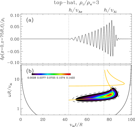
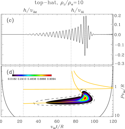
Figure 3: Density perturbations $\delta\rho$ at a distance $h=75R$ from the impulsive source along the axis of a coronal slab with top-hat profiles. The left and right columns pertain to a density contrast $\rho_{\rm i}/\rho_{\rm e}$ of $3$ and $10$, respectively. In addition to the temporal evolution (the upper row), the corresponding Morlet spectra are also shown (lower). The left and right vertical axes in the lower row represent the angular frequency $\omega$ and period $P$, respectively. Furthermore, the black solid curves represent the cone of influence, and the area inside the dashed contour indicates where the Morlet power exceeds the $95\%$ confidence level. The dotted vertical lines correspond to the arrival times of wavepackets traveling at the internal and external Alfvén speeds as labeled. The yellow curves represent $\omega-h/v_{\rm gr}$ as found from the eigenmode analysis, with the transverse order increasing from bottom to top.

Figure 3 displays the temporal evolution (the upper row) and the pertinent Morlet spectra (lower) of the density perturbations $\delta\rho$ sampled at a distance $h=75R$ along the slab axis for both a density contrast $\rho_{\rm i}/\rho_{\rm e}=3$ (the left column) and $10$ (right). In the lower row, the left (right) vertical axis represents the angular frequency $\omega$ (the period $P$). The Morlet spectra are created by using the standard wavelet toolkit devised by Torrence & Compo (1998), and the dashed contours represent the $95\%$ confidence level computed by assuming a white-noise process for the mean background spectrum. The dotted vertical lines correspond to the arrival times of wavepackets traveling at the internal and external Alfvén speeds, i.e., $v_{\rm Ai}$ and $v_{\rm Ae}$. The yellow curves represent $\omega$ as a function of $h/v_{\rm gr}$, replotted with the numerical results already given in the lower row of Fig. 2. For these $\omega-h/v_{\rm gr}$ curves, the corresponding transverse harmonic number increases from bottom to top.

Consider the lower row first. The first impression is that the Morlet spectra are well organized by the group speed curves. In particular, it is clear that with the present choice of the initial perturbation, wavepackets corresponding to the fundamental transverse mode (with $l=1$) dominate the signals. Figure 3d shows the typical shape of “crazy tadpoles”, for which the broad head corresponds to the portion of the $v_{\rm gr}-k$ curve where the local minimum is embedded. This indicates that wavepackets corresponding to that portion can receive a substantial fraction of the energy contained in the initial perturbation, and the subsequent superposition of multiple wavepackets with the same group speed but different frequencies can account for both the enhancement of the Morlet power and the broadening in frequency coverage. Note that this is in close agreement with the heuristic reasoning by Edwin & Roberts (1986). The Morlet spectrum in Fig. 3b, albeit also looking like a “crazy tadpole”, is somehow different in that the strongest power does not enclose the group speed minimum. The initial perturbation can still distribute a certain amount of energy to wavepackets beyond the group speed minimum, but this fraction is less significant and the superposition of wavepackets is not as clear as in Fig. 3d. Nonetheless, this fraction is still substantial enough to show up, resulting in the broadening in frequency coverage and the consequent appearance of a broad head. Given that a fixed initial perturbation is adopted in this present study, the difference between Figs. 3b and 3d indicates the importance of the density contrast in determining how the energy contained in the initial perturbation is distributed to different frequency ranges along the group speed curves.

The observational implications of Figs. 3b and 3d are as follows. First, the $\omega-h/v_{\rm gr}$ curves thread the narrow tails rather than bordering them from below. As a consequence, in principle the longest period $P_{\rm Max}$ that can be resolved in the crazy tadpoles cannot be attributed to $P_{\rm c}$, the longest period that trapped modes can theoretically attain. However, $P_{\rm Max}$ differs from $P_{\rm c}$ only marginally. Given the practical uncertainties in determining $P_{\rm Max}$ (the longest period), it should be fine if one equates $P_{\rm c}$ (the cutoff period in the trapped regime) to $P_{\rm Max}$ in the crazy tadpoles as found in, say, optical observations at total eclipses (e.g., Williams et al. 2001, 2002). Second, the timescales associated with the strongest power do not differ much from $P_{\rm c}$ and amount to a couple of the transverse Alfvén times. Note that the cutoff period $P_{\rm c}=2\pi/(k_{\rm c,1}v_{\rm Ae})=4(R/v_{\rm Ai})\sqrt{1-\rho_{\rm e}/\rho_{\rm i}}$ for top-hat profiles, as indicated by Equation (19). This means that the present crazy tadpoles can be most readily found in high-cadence measurements made in, say, radio passbands.

4 PHILOSOPHY FOR A COMPARATIVE STUDY BETWEEN THE SLAB AND CYLINDRICAL GEOMETRIES

Comparing Figure 3 with Figure 3 in paper I indicates that they are remarkably similar. In fact, repeating the computations presented in paper I for the slab geometry, we find that the same can be said for all the Morlet spectra that are obtained. Regardless of geometry, the Morlet spectra are all shaped by the $\omega-h/v_{\rm gr}$ curves, which in turn derive from the frequency dependence of the axial group speed of trapped sausage modes. In this regard, there is no point to present the Morlet spectra again: the slab results can be well anticipated with their cylindrical counterparts as long as we can quantify the difference that a slab geometry introduces to the group speed curves. Therefore, for the group speed curves and Morlet spectra pertinent to the slab geometry, we refer the readers to the relevant figures in paper I as listed in the last two columns in Table 1. In what follows we examine the differences between the two geometries of the parameters that characterize the group speed curves.

4.1 Comparison of Cutoff Wavenumbers

Common to both geometries, with the help of Kneser’s oscillation theorem, one can analytically establish that cutoff wavenumbers ($k_{{\rm c},l}$) exist only when the transverse density profile drops sufficiently rapidly at large distances. This was shown by Lopin & Nagorny (2015b) for the cylindrical case (also see paper I for numerical demonstrations), and by Lopin & Nagorny (2015a, hereafter LN15) for the slab geometry. If $f(x)$ tends to zero in the way described by Equation (7), then this translates into that $k_{{\rm c},l}$ exists only when $\mu_{\infty}\geq 2$. Our numerical results with BVPSuite agree with this analytical expectation. In fact, we can further demonstrate that when cutoff wavenumbers exist, they should be of the form

$$\displaystyle k_{{\rm c},l}R=\frac{d_{l}}{\sqrt{\rho_{\rm i}/\rho_{\rm e}-1}}~{},$$ (28)

where $d_{l}$ is a dimensionless parameter that measures how well a slab can trap sausage modes in terms of their axial wavelengths. It can be readily shown that $d_{l}$ possesses no dependence on the density contrast $\rho_{\rm i}/\rho_{\rm e}$. To see this, we note that the terms in the parentheses in Equation (11) can be reformulated as $k^{2}(v_{\rm ph}^{2}/v_{\rm A}^{2}-1)$, which reads $k_{{\rm c},l}^{2}(\rho/\rho_{\rm e}-1)$ at cutoffs given that $v_{\rm ph}=v_{\rm Ae}$. With $\rho(x)$ given by Equation (1), this then yields $k_{{\rm c},l}^{2}(\rho_{\rm i}/\rho_{\rm e}-1)f(x)$. As a result, $k_{{\rm c},l}\sqrt{\rho_{\rm i}/\rho_{\rm e}-1}$ does not depend on the density contrast any more but is solely determined by $f(x)$. Repeating the same practice for Equation (8) in paper I, one sees that Equation (28) also holds for the cylindrical geometry. Therefore, common to both geometries, Equation (28) suggests that $k_{{\rm c},l}$ always decreases with $\rho_{\rm i}/\rho_{\rm e}$ for a given $l$ for any profile describable by Equation (1).

The specific values of $d_{l}$, however, are geometry dependent. Take the top-hat profile, which is an exemplary realization for $\mu_{\infty}=\infty$. Equation (19) indicates that $d_{l}=(l-1/2)\pi$ for a slab geometry whereas $d_{l}=j_{0,l}$ for a cylindrical one (see, e.g., Equation 15 in paper I). Here $j_{0,l}$ is the $l$-th zero of $J_{0}$ ($l=1,2,3,\cdots$). Listed in the second row of Table 2 are some specific values of $d_{l}$ for the first several transverse harmonic numbers. One sees that $d_{l}$ is always larger for a given $l$ in the cylindrical case, which is understandable given that $j_{0,l}$ can be well approximated by $(l-1/4)\pi$ (see Equation 9.2.1 in Abramowitz & Stegun 1972, hereafter AS). Table 2 also compares another two profiles, for which $d_{l}$ can be analytically found in the slab geometry. These two profiles, examined in Appendices A and B, are not analytically tractable in the cylindrical geometry and were not examined in paper I. The pertinent values for $d_{l}$ are found with BVPSuite.

It is also possible to offer some rather generic analysis for the cutoff wavenumbers when $\mu_{\infty}=2$. In the cylindrical case, Lopin & Nagorny (2015b) showed that $d_{l}=1$. Closely following the approach therein, we now examine what happens in the slab geometry. By noting that $m=0$ at the cutoff wavenumber, one finds that Equation (11) at large distances is approximately

$$\frac{{\rm d}^{2}\tilde{\xi}}{{\rm d}x^{2}}+\frac{DR^{2}}{x^{2}}\tilde{\xi}=0~{}.$$ (29)

The solution to this equation is in the form

$$\displaystyle\tilde{\xi}\propto\left(x/R\right)^{1/2}\sin\left[\left(\ln\frac{x}{R}\right)\sqrt{DR^{2}-\frac{1}{4}}\right].$$ (30)

For waves to be trapped, $\tilde{\xi}$ should be non-oscillatory when $x/R\rightarrow\infty$, meaning that $DR^{2}-1/4=0$. Given that now $DR^{2}=k_{{\rm c},l}^{2}R^{2}(\rho_{\rm i}/\rho_{\rm e}-1)$, one finds

$$k_{{\rm c},l}R=\displaystyle\frac{1/2}{\sqrt{\rho_{\rm i}/\rho_{\rm e}-1}}~{}.$$ (31)

In other words, $d_{l}=1/2$, which does not depend on $l$. Furthermore, the derivation shown above indicates that $d_{l}$ does not depend on the details of $f(x)$ either. It always reads $1/2$ as long as $f(x)\approx(x/R)^{-2}$ at large $x$. Therefore, it is not surprising to see that Equation (31) was shown by LN15 to hold for an $f(x)$ being $1/(1+x/R)^{2}$, in which case an analytical DR can be found (see also appendix C).

The profiles examined so far suggest that $d_{l}$ for arbitrary $l$ is larger in the cylindrical case. Physically speaking, this means that magnetic slabs can trap sausage waves with longer axial wavelengths than magnetic cylinders. When $f(x)\approx(x/R)^{-2}$, we have shown that this is true regardless of the details of $f(x)$ close to the structure. However, it remains to be examined as to how $d_{l}$ behaves for other cases. Specializing to the “inner $\mu$” profile, for instance, we still need to find out how $d_{l}$ in the slab case differs from its cylindrical counterpart when $\mu_{0}$ varies (see Table 1).

4.2 Comparison of the Behavior of the Group Speed Curves at Large Wavenumbers

For both geometries and for all the profiles given by Equations (2) to (4), we find that the axial phase speeds at large $kR$ take the form

$$\frac{v_{\rm ph}^{2}}{v_{\rm Ai}^{2}}\approx 1+\displaystyle\left(\frac{c_{l}}{kR}\right)^{\beta}.$$ (32)

The exponent $\beta$ is geometry independent, and is entirely determined by the steepness of $f$ at the structure axis. In terms of $\mu_{0}$ (see Equation 7), we find that

$$\displaystyle\beta=\frac{2\mu_{0}}{\mu_{0}+2}.$$ (33)

We further find that the constant $c_{l}$ is of the form

$$\displaystyle c_{l}=h_{l}\left(1-\frac{\rho_{\rm e}}{\rho_{\rm i}}\right)^{1/\mu_{0}}~{}.$$ (34)

where $h_{l}$ does not depend on $\rho_{\rm i}/\rho_{\rm e}$ but is geometry dependent. Equation (32) was found through an extensive parameter study with BVPSuite, and was also given in paper I for the cylindrical geometry. However, it was not mentioned therein that $c_{l}$ takes the form given by Equation (34). Actually, this apparently involved form is inspired by the analytical analysis enabled by the mathematical simplicity for the slab geometry. For the top-hat profile pertinent to $\mu_{0}=\infty$, Equation (26) indicates that $c_{l}=l\pi$. There is no need to distinguish between $\mu$ and $\mu_{0}$ for the “inner $\mu$” profile. In this case, for $\mu=2$ and $\mu=1$, Section 7.1 indicates that the dependence of $c_{l}$ on the density contrast reads $(1-\rho_{\rm e}/\rho_{\rm i})^{1/2}$ and $(1-\rho_{\rm e}/\rho_{\rm i})$, respectively.

The importance of Equation (32) is that it largely determines whether the $v_{\rm gr}-k$ curves are monotonical. This is because the axial group speed at large $kR$ is given by

$$\displaystyle\frac{v_{\rm gr}^{2}}{v_{\rm Ai}^{2}}\approx 1+\left(1-\beta\right)\left(\frac{c_{l}}{kR}\right)^{\beta}~{}.$$ (35)

It follows from Equation (33) that $\beta>1$ ($\beta<1$) when $\mu_{0}>2$ ($\mu_{0}<2$), meaning that $v_{\rm gr}$ approaches $v_{\rm Ai}$ from above (below) asymptotically. Now that $v_{\rm gr}$ always decreases first with increasing $k$, this means that the $v_{\rm gr}-k$ curve is definitely nonmonotonical when $\mu_{0}>2$ and is very likely to be monotonical when $\mu_{0}<2$.

Given the importance of Equation (32), we have also examined another two profiles that can be approximated by $f(x)\approx 1-(x/R)^{\mu_{0}}$ when $x\ll R$. Appendix A examines an $f(x)$ being $\exp(-x/R)$, pertinent to $\mu_{0}=1$. The behavior of $v_{\rm ph}$ at large $kR$ is in exact agreement with what we found for the “inner $\mu$” profile with $\mu=1$. In Appendix B, $f(x)$ is described by ${\rm sech}^{2}(x/R)$, pertinent to $\mu_{0}=2$. The asymptotic behavior of $v_{\rm ph}$ is found to agree exactly with the results for the “inner $\mu$” profile with $\mu=2$. These two profiles are distinct from those in the main text in that they do not follow the form given by Equation (7) at large $x$. This means that the validity of Equation (32) does not depend on the details of $f(x)$ away from the slab axis. In fact, the same can be said also for the cylindrical case. Examining coronal tubes with these two profiles, albeit now numerically with BVPSuite, we find that Equations (32) to (34) also hold. Furthermore, the comparison between the two geometries for these two profiles indicate that $h_{l}$ is geometry dependent (see Table 3).

All the above-mentioned results enable us to conjecture that

Conjecture 1

The phase speeds for sausage waves at large axial wavenumbers can be approximated by Equation (32) for any $f(x)$ that is approximately $1-(x/R)^{\mu_{0}}$ when $x/R\ll 1$. Here $\beta$ and $c_{l}$ are given by Equations (33) and (34), respectively. Equation (32) is valid for both the slab and cylindrical geometries, barring the trivial difference that $x$ should be interpreted as the radial distance from the tube axis in the latter. Note, however, that $h_{l}$ is geometry dependent.

Conjecture 1 is supported by all the analytical results in both paper I and this study. However, while mathematically simpler, compact closed-form DRs can be found for trapped sausage waves only for a handful of density profiles even in the slab geometry. Therefore in what follows we will first show that Conjecture 1 is also supported by all the numerical results for profiles given by Equations (2) to (4). By doing this, we will also be able to address the difference in the asymptotic behavior of the axial phase speed in the two geometries. For this purpose, only $h_{l}$ needs to be compared.

5 CORONAL SLABS WITH “$\mu$ POWER” PROFILES

This section examines the “$\mu$ power” profiles as given by Equation (2). We will start with an examination of the particular case with $\mu=1$, for which an analytical treatment is possible.

5.1 Analytical Results for $\mu=1$

The case with $\mu=1$ has already been examined by LN15. The solution to Equation (11) can be shown to have the form

$$\tilde{\xi}\propto W_{\nu,1/2}(X),$$

where $X=2m(x+R)$, and $W_{\cdot,\cdot}(\cdot)$ is Whittaker’s W function (see section 13.1 in AS). In addition,

$$\nu=\displaystyle\frac{\bar{D}}{2\bar{m}}~{}.$$ (36)

The DR is given simply by the requirement that $\tilde{\xi}(x=0)=0$, resulting in

$$W_{\nu,1/2}(2mR)=0~{}.$$ (37)

No cutoff wavenumber exists for sausage modes of any transverse harmonic number $l$, given that $f(x)$ decreases less rapidly than $x^{-2}$ at large $x$. When $kR\rightarrow 0$, it turns out that $\nu\rightarrow l$. The definition of $\nu$ then yields an equation quadratic in $\omega^{2}$. Solving this equation for $\omega^{2}$, one finds that

$$\frac{v_{\rm ph}^{2}}{v_{\rm Ae}^{2}}\approx 1-\left(\frac{\rho_{\rm i}/\rho_{\rm e}-1}{2l}\right)^{2}\left(kR\right)^{2}~{},$$ (38)

and

$$\frac{v_{\rm gr}^{2}}{v_{\rm Ae}^{2}}\approx 1-3\left(\frac{\rho_{\rm i}/\rho_{\rm e}-1}{2l}\right)^{2}\left(kR\right)^{2}~{}.$$ (39)

Note that LN15 also considered this situation, and an expression for $v_{\rm ph}$ at small $kR$ was given by Equation (49) therein. However, a typo is present there in that $1/\chi$ (or $\rho_{\rm i}/\rho_{\rm e}$ with our notations) should be replaced by $\rho_{\rm i}/\rho_{\rm e}-1$.

The analytical treatment up to this point was already done by LN15. Let us offer some new results by finding the asymptotic expressions for $v_{\rm ph}$ and $v_{\rm gr}$ when $kR\rightarrow\infty$. To start, let us note that $v_{\rm ph}$ approaches $v_{\rm Ai}$ from above and both $mR$ and $\nu$ approach infinity. Let $\chi$ denote $mR/(2\nu)=m^{2}R^{2}/D$. It is easy to show that $\chi$ approaches unity from below, namely $\chi\rightarrow 1^{-}$. Now to evaluate the DR (37), one needs the asymptotic expansion for $W_{\nu,1/2}(4\nu\chi)$ at large $\nu$, which was given on page 412 in Olver (1997) and is too lengthy to be included here. Fortunately, for our purpose $W_{\nu,1/2}(4\nu\chi)$ is dominated by a term proportional to ${\rm Ai}[(4\nu)^{2/3}\zeta]$ where ${\rm Ai}$ is Airy’s function, and $\zeta$ denotes the solution to the following equation

$$\displaystyle\frac{4}{3}\left(-\zeta\right)^{3/2}=\arccos\left(\chi^{1/2}\right)-\left(\chi-\chi^{2}\right)^{1/2}~{}.$$ (40)

This means that the solution to the DR can be approximated by

$$\displaystyle(4\nu)^{2/3}\zeta\approx a_{l}\approx-\left[\frac{3\left(4l-1\right)\pi}{8}\right]^{2/3}~{},$$ (41)

where $a_{l}$ denotes the $l$-th zero of ${\rm Ai}$ and the second approximation is accurate to within $2\%$ (see AS, page 450). Using the definition of $\nu$, one finds that

$$\displaystyle\zeta\approx a_{l}(4\nu)^{-2/3}=a_{l}\left(2kR\sqrt{1-\frac{\rho_{\rm e}}{\rho_{\rm i}}}\right)^{-2/3}~{}.$$ (42)

Now let $\chi=1-\delta$ where $0<\delta\ll 1$. Taylor-expanding the RHS of Equation (40) and keeping terms up to $\delta^{3/2}$, one finds that $\delta=-2^{2/3}\zeta$. Furthermore, let $(v_{\rm ph}/v_{\rm Ai})^{2}=1+\gamma$ where $\gamma$ is small and positive. Plugging $v_{\rm ph}^{2}$ into the definitions of $m$ and $\nu$, one finds that $\chi=1-\gamma/(1-\rho_{\rm e}/\rho_{\rm i})$, meaning that $\gamma=(1-\rho_{\rm e}/\rho_{\rm i})\delta=-(1-\rho_{\rm e}/\rho_{\rm i})2^{2/3}\zeta$. Given Equations (41) and (42), one then finds that

$$\displaystyle\frac{v_{\rm ph}^{2}}{v_{\rm Ai}^{2}}\approx 1+\left[\frac{3\left(4l-1\right)\pi(1-\rho_{\rm e}/\rho_{\rm i})}{8kR}\right]^{2/3}~{},$$ (43)

and

$$\displaystyle\frac{v_{\rm gr}^{2}}{v_{\rm Ai}^{2}}\approx 1+\frac{1}{3}\left[\frac{3\left(4l-1\right)\pi(1-\rho_{\rm e}/\rho_{\rm i})}{8kR}\right]^{2/3}~{}.$$ (44)

This means that both $v_{\rm ph}$ and $v_{\rm gr}$ eventually approach $v_{\rm Ai}$ from above when $kR$ increases.

5.2 Comparison with the Cylindrical Results

Let us start by noting that there is no need to distinguish between $\mu$ and $\mu_{0}$ or $\mu$ and $\mu_{\infty}$ for this family of profiles. In other words, $\mu_{0}=\mu$ and $\mu_{\infty}=\mu$.

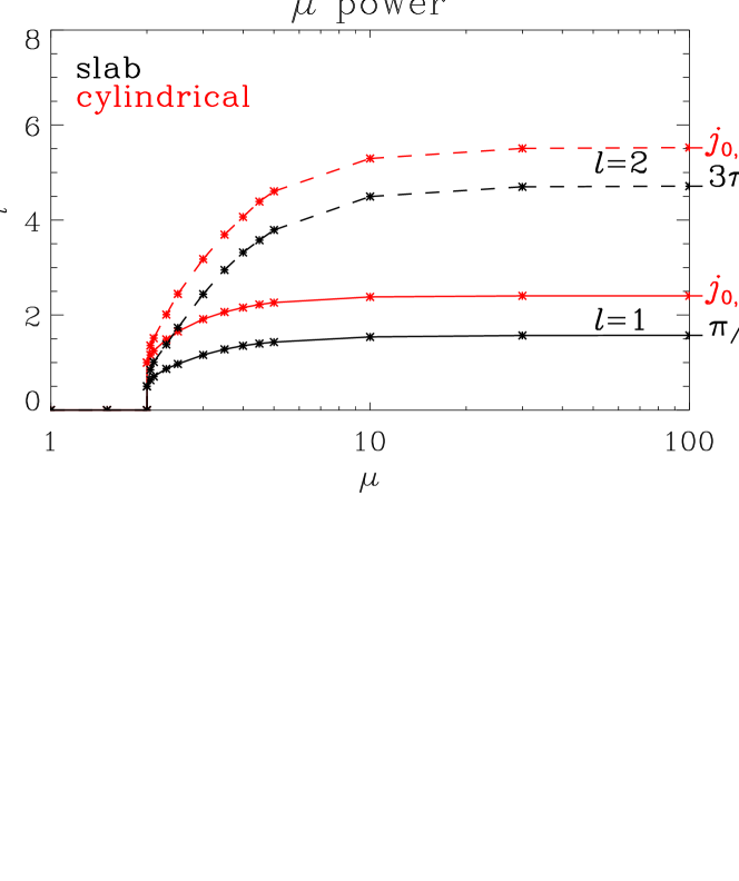
Figure 4: Dependence of $d_{l}$ on $\mu$ for coronal structures with “$\mu$ power” profiles. Here $d_{l}$ is related to cutoff axial wavenumbers $k_{{\rm c},l}$ by $d_{l}=(k_{{\rm c},l}R)\sqrt{\rho_{\rm i}/\rho_{\rm e}-1}$ and does not depend on the density contrast $\rho_{\rm i}/\rho_{\rm e}$. Both coronal slabs (the black curves) and tubes (red) are examined. The solid and dashed curves represent the transverse fundamental mode (with transverse order $l=1$) and its first harmonic ($l=2$), respectively. The horizontal bars present the values of $d_{l}$ expected for top-hat profiles. Note that for “$\mu$ power” profiles, $f(x)$ conforms to $1-(x/R)^{\mu_{0}}$ when $x/R\ll 1$ and $(x/R)^{-\mu_{\infty}}$ when $x/R\gg 1$, with $\mu_{0}=\mu_{\infty}=\mu$. See text for details.

As indicated by Equation (28), $d_{l}$ is entirely determined by geometry for a given $f(x)$. Figure 4 compares the values of $d_{l}$ in the slab geometry (the black curves) with those in the cylindrical one (red) for an extensive range of the $\mu$ values. The solid curves are for the transverse fundamental mode ($l=1$), whereas the dashed ones are for the first transverse harmonic ($l=2$). Given by the horizontal bars are the analytical expectations for $d_{l}$ in the top-hat case, namely $\mu=\mu_{\infty}\rightarrow\infty$. One sees that $d_{l}$ is nonzero only when $\mu=\mu_{\infty}\geq 2$. Furthermore, while in general $d_{l}$ is $\mu$ dependent for a given geometry, it is not so when $\mu=2$. Comparing the black and red curves, one also sees that $d_{l}$ is always larger in the cylindrical geometry at arbitrary $\mu$, indicating that magnetic slabs with “$\mu$ power” profiles can trap sausage waves with longer axial wavelengths.

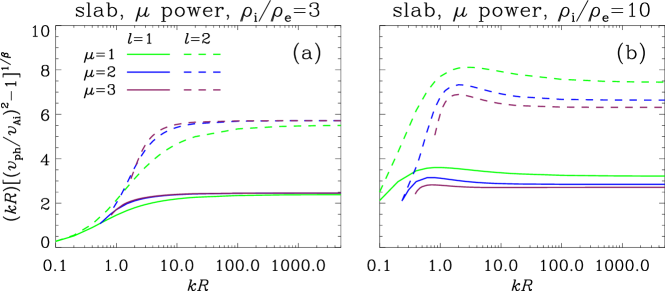
Figure 5: Axial phase speed $v_{\rm ph}$ as a function of axial wavenumber $k$ for trapped sausage waves in coronal slabs with “$\mu$ power” profiles. The left (right) panel pertains to a density contrast $\rho_{\rm i}/\rho_{\rm e}$ of $3$ ($10$). Both the transverse fundamental mode (with transverse order $l=1$, the solid curves) and its first harmonic ($l=2$, dashed) are examined. The results for a number of values of $\mu$ are shown by the curves in different colors. Note that the combination $(kR)[(v_{\rm ph}/v_{\rm Ai})^{2}-1]^{1/\beta}$ is plotted rather than $v_{\rm ph}$ itself, where $\beta=2\mu/(\mu+2)$. Note further that for “$\mu$ power” profiles, $f(x)$ conforms to $1-(x/R)^{\mu_{0}}$ when $x/R\ll 1$ and $(x/R)^{-\mu_{\infty}}$ when $x/R\gg 1$, with $\mu_{0}=\mu_{\infty}=\mu$. See text for details.

Now turn to the asymptotic behavior of the axial phase speeds $v_{\rm ph}$ at large axial wavenumbers ($kR$). Before examining the differences in the two geometries, we first employ the slab computations to demonstrate that Equation (32) to (34) indeed hold. To do this, we have evaluated the dependence on $kR$ of $(kR)(v_{\rm ph}^{2}/v_{\rm Ai}^{2}-1)^{1/\beta}$ for an extensive range of $[l,\mu,\rho_{\rm i}/\rho_{\rm e}]$, where $\beta$ is given by Equation (33) and we take $\mu_{0}=\mu$. A subset of this parameter study is shown in Figure 5, where we present how $(kR)(v_{\rm ph}^{2}/v_{\rm Ai}^{2}-1)^{1/\beta}$ depends on $kR$ for a density contrast $\rho_{\rm i}/\rho_{\rm e}=3$ (the left panel) and $\rho_{\rm i}/\rho_{\rm e}=10$ (right). The examined combinations of $[l,\mu$] are represented with different linestyles and colors as labeled. The point here is that for any given $[l,\mu]$, the curves pertinent to both density contrasts tend to some asymptotic values for sufficiently large $kR$, meaning that Equation (32) is indeed valid. In fact, this is how we determine the constant $c_{l}$. Comparing the dashed with the solid curves, one sees that $c_{l}$ is different for different $l$. Furthermore, $c_{l}$ also depends on $\mu$ at a given $\rho_{\rm i}/\rho_{\rm e}$, even though this dependence is rather weak for a modest density contrast $\rho_{\rm i}/\rho_{\rm e}=3$ (see Figure 5a). When both $l$ and $\mu$ are fixed, $c_{l}$ is different at different values of $\rho_{\rm i}/\rho_{\rm e}$ as can be seen if one compares, say, the asymptotic value that the blue dashed curve attains in Figure 5a with that in Figure 5b.

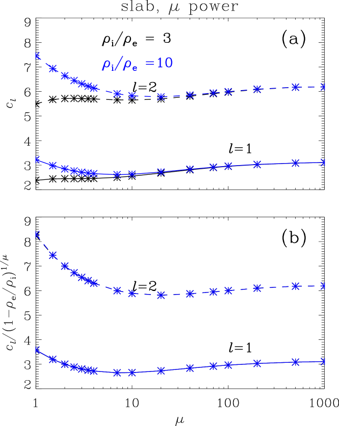
Figure 6: Dependence on $\mu$ of $c_{l}$ (the upper panel) and $c_{l}/(1-\rho_{\rm e}/\rho_{\rm i})^{1/\mu}$ (lower) for coronal slabs with “$\mu$ power” profiles. The solid (dashed) curves are for the transverse fundamental mode ($l=1$) and its first harmonic ($l=2$), respectively. Two density contrasts $\rho_{\rm i}/\rho_{\rm e}$ are examined, one being $3$ (the black curves) and the other being $10$ (blue). Note that for “$\mu$ power” profiles, $f(x)$ conforms to $1-(x/R)^{\mu_{0}}$ when $x/R\ll 1$ and $(x/R)^{-\mu_{\infty}}$ when $x/R\gg 1$, with $\mu_{0}=\mu_{\infty}=\mu$. See text for details.

That $c_{l}$ depends on the combination $[l,\mu,\rho_{\rm i}/\rho_{\rm e}]$ is made more evident in Figure 6a, where $c_{l}$ is shown as a function of $\mu$ for both $l=1$ (the solid curves) and $l=2$ (dashed) and for both $\rho_{\rm i}/\rho_{\rm e}=3$ (the black curves) and $\rho_{\rm i}/\rho_{\rm e}=10$ (blue). One sees that $c_{l}$ increases with $l$ regardless of $\mu$ or $\rho_{\rm i}/\rho_{\rm e}$. Likewise, $c_{l}$ increases with $\rho_{\rm i}/\rho_{\rm e}$ at a given $l$, and this tendency becomes increasingly weak with $\mu$. This rather complicated dependence on $\rho_{\rm i}/\rho_{\rm e}$ makes the comparison of the asymptotic behavior between the two geometries rather cumbersome. Fortunately, this dependence can be removed if one examines $c_{l}/(1-\rho_{\rm e}/\rho_{\rm i})^{1/\mu}$. Shown in Figure 6b, this ratio at a given $l$ becomes solely determined by $\mu$ as evidenced by the fact that the blue and black curves coincide. This means that Equation (34) holds. Repeating the same practice involved in Figures 5 and 6 for the cylindrical case, we find exactly the same behavior.

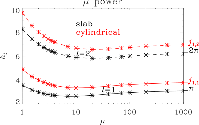
Figure 7: Comparison of the dependence of $h_{l}$ on $\mu$ for trapped sausage waves in coronal slabs (the black curves) and tubes (red). The solid and dashed curves are for the transverse fundamental mode ($l=1$) and its first harmonic ($l=2$), respectively. The horizontal bars represent the values of $h_{l}$ expected for top-hat profiles. Note that for “$\mu$ power” profiles, $f(x)$ conforms to $1-(x/R)^{\mu_{0}}$ when $x/R\ll 1$ and $(x/R)^{-\mu_{\infty}}$ when $x/R\gg 1$, with $\mu_{0}=\mu_{\infty}=\mu$. See text for details.

Now we are in a position to compare how the asymptotic behavior of the axial phase speed differs in different geometries. Figure 7 shows $h_{l}=c_{l}/(1-\rho_{\rm e}/\rho_{\rm i})^{1/\mu}$ as a function of $\mu$ for both the slab (the black curves) and cylindrical (red) geometries and for both $l=1$ (the solid curves) and $l=2$ (dashed). The horizontal bars represent the top-hat results pertaining to $\mu\rightarrow\infty$, in which case $h_{l}=l\pi$ ($h_{l}=j_{1,l}$) for the slab (cylindrical) geometry (see Table 3). Consider the slab results as given by the black curves. For “$\mu$ power” profiles, the only analytically tractable case happens when $\mu=1$, for which Equation (43) offers an explicit expression for $h_{l}$. Evaluating this $h_{l}$ yields that $h_{1}=3.53$ and $h_{2}=8.25$, which are in close agreement with the numerical results. With increasing $\mu$, one sees that $h_{l}$ decreases first before increasing toward the top-hat results eventually. This behavior is also seen in the cylindrical computations shown by the red curves. It is just that $h_{l}$ is always larger.

6 CORONAL SLABS WITH “OUTER $\mu$” PROFILES

This section examines coronal slabs with “outer $\mu$” profiles as given by Equation (3). For this family of profiles, closed-form DRs can be found for $\mu=1$ and $\mu=2$. In what follows, we will start with an examination on these two particular choices of $\mu$ and see what we can expect.

6.1 Analytical Results for $\mu=1$ and $\mu=2$

Let us start with the case where $\mu=1$. The solution to Equation (11) in the outer portion can be shown to have the form

$$\tilde{\xi}\propto W_{\nu,1/2}(X),$$

where $X=2mx$, and $\nu$ is also defined by Equation (36). With $\tilde{\xi}$ expressible in terms of $\sin(nx)$ in the inner portion, the DR reads

$$nR\displaystyle\cot(nR)=mR-\nu-\displaystyle\frac{W_{\nu+1,1/2}(2mx)}{W_{\nu,1/2}(2mx)}~{}.$$ (45)

We have used the fact that

$$\frac{{\rm d}}{{\rm d}X}W_{\nu,1/2}(X)=\left(\frac{1}{2}-\frac{\nu}{X}\right)W_{\nu,1/2}(X)-\frac{W_{\nu+1,1/2}(X)}{X}~{}.$$

No cutoff wavenumbers exist because $f(x)$ at large distances drops less rapidly than $(x/R)^{-2}$. Some approximate results can be found in the limiting cases where $k\rightarrow 0$ or $k\rightarrow\infty$. When $k\rightarrow 0$, it turns out that $\nu\rightarrow l$ for transverse order $l$ with $l=1,2,3,\cdots$. Actually this is what happens for “$\mu$ power” profiles with $\mu=1$, meaning that $v_{\rm ph}$ and $v_{\rm gr}$ can still be approximated by Equations (38) and (39), respectively. On the other hand, when $kR$ approaches infinity, the RHS of Equation (45) tends to infinity. As happens in the top-hat case, the phase and group speeds for trapped modes of transverse order $l$ can still be approximated by Equations (26) and (27), respectively.

Now consider the case where $\mu=2$. The solution to Equation (11) in the outer portion can be shown to have the form

$$\tilde{\xi}\propto K_{\nu}(X),$$

where $X=mx$ and $K_{\nu}$ is modified Bessel’s function of the second kind with

$$\displaystyle\nu=\sqrt{\frac{1}{4}-\bar{D}}~{}.$$ (46)

With $\tilde{\xi}$ expressible in terms of $\sin(nx)$ in the inner portion, the DR reads

$$\displaystyle(nR)\cot(nR)=\frac{1}{2}-\nu-(mR)\displaystyle\frac{K_{\nu-1}(mR)}{K_{\nu}(mR)}~{}.$$ (47)

In this case, the cutoff wavenumbers are still given by Equation (31). One then sees that $\nu\to 0$ at the cutoff because $\bar{D}=1/4$. Moving away from this cutoff, $v_{\rm ph}k$ increases with $k$, meaning that $\nu$ becomes purely imaginary (see DLMF 2016, section 10.45, for a discussion of $K_{\nu}$ of imaginary order). As is the case for $\mu=1$, the RHS of Equation (47) grows unbounded when $kR$ approaches infinity. This means that once again $v_{\rm ph}$ and $v_{\rm gr}$ can be approximated by Equations (26) and (27), respectively.

6.2 Comparison with the Cylindrical Results

Note that for this family of profiles, $\mu_{0}$ is identically infinite and $\mu_{\infty}$ is indistinguishable from $\mu$. In other words, $\mu_{0}\equiv\infty$ and $\mu_{\infty}=\mu$.

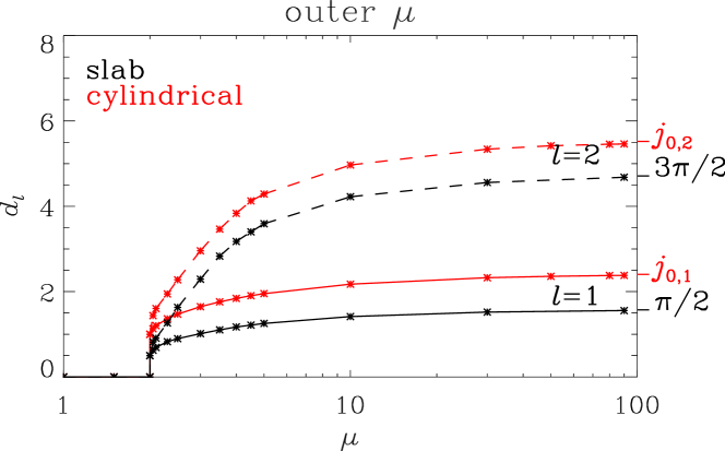
Figure 8: Similar to Figure 4 but for coronal slabs with “outer $\mu$” profiles. Note that for this family of profiles, $f(x)$ conforms to $1-(x/R)^{\mu_{0}}$ when $x/R\ll 1$ and $(x/R)^{-\mu_{\infty}}$ when $x/R\gg 1$, with $\mu_{0}=\infty$ and $\mu_{\infty}=\mu$.

Figure 8 shows, in a format similar to Figure 4, the dependence of $d_{l}$ on $\mu$ for both the slab (the black curves) and cylindrical (red) geometries. Despite some quantitative difference, the curves look remarkably similar to their counterparts for the “$\mu$ power” family of profiles. In particular, ones sees that $d_{l}$ is identically zero for $\mu<2$ but increases with $\mu$ before leveling off. Furthermore, the case with $\mu=2$ is special in the sense that $d_{l}$ does not depend on $l$. A comparison between the curves in the same linestyle but in different colors shows that $d_{l}$ is always larger in the cylindrical case.

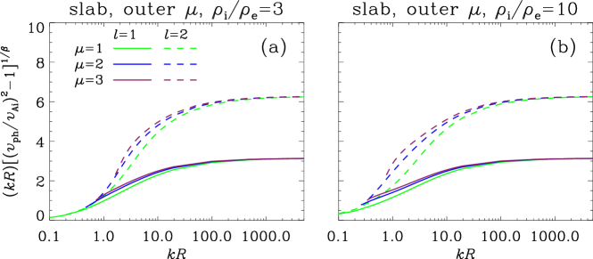
Figure 9: Similar to Figure 5 but for “outer $\mu$” profiles. Note that for this family of profiles, $f(x)$ conforms to $1-(x/R)^{\mu_{0}}$ when $x/R\ll 1$ and $(x/R)^{-\mu_{\infty}}$ when $x/R\gg 1$, with $\mu_{0}=\infty$ and $\mu_{\infty}=\mu$. A $\mu_{0}$ being infinite is employed to evaluate $\beta$, resulting in $\beta=2\mu_{0}/(\mu_{0}+2)=2$. See text for details.

Let us examine whether Equations (32) to (34) hold, still with the slab computations. To do this, we can still examine the wavenumber dependence of $(kR)(v_{\rm ph}^{2}/v_{\rm Ai}^{2}-1)^{1/\beta}$, it is just that now $\beta=2$ given that $\mu_{0}=\infty$ (see Equation 33). Figure 9 shows how $(kR)(v_{\rm ph}^{2}/v_{\rm Ai}^{2}-1)^{1/\beta}$ varies with $kR$ for a number of combinations $[l,\mu,\rho_{\rm i}/\rho_{\rm e}]$ as labeled. Similar to the “$\mu$ power” profiles (see Figure 5), for sufficiently large $kR$ all the curves tend to some constant, which we take as $c_{l}$. However, in this case $c_{l}$ does not depend on the density contrast any more. In both Figures 9a and 9b, we find that $c_{l}=l\pi$, which is the result expected for top-hat profiles (see Table 3). In fact, for $\mu=1$ and $\mu=2$, we have analytically shown that $h_{l}$ attains the top-hat values. That $c_{l}$ does not depend on $\rho_{\rm i}/\rho_{\rm e}$ or $\mu$ lends further support to Conjecture 1: Equation (34) indicates that $c_{l}$ is indistinguishable from $h_{l}$ and is therefore entirely determined by geometry for a $\mu_{0}$ being infinite. Furthermore, the computations given in Figure 9 also shows that the behavior of $f(x)$ away from the slab axis does not play a role in determining $h_{l}$. Repeating the computations for the cylindrical geometry yields exactly the same behavior. It is just that now $c_{l}$ or equivalently $h_{l}$ reads $j_{1,l}$ (see Table 3).

7 CORONAL SLABS WITH “INNER $\mu$” PROFILES

This section examines “inner $\mu$” profiles as given by Equation (4). In this case, compact closed-form DRs for sausage modes can be found when $\mu=1$ and $2$.

7.1 Analytical Results for $\mu=1$ and $\mu=2$

Let us start with the case where $\mu=1$. The solution to Equation (11) in the inner portion is a linear combination of Airy’s functions ${\rm Ai}(X)$ and ${\rm Bi}(X)$, where

$$\displaystyle X=\frac{-\bar{n}^{2}+\bar{D}^{2}(x/R)}{\bar{D}^{2/3}}~{}.$$ (48)

Given that $\tilde{\xi}(x=0)=0$, the Lagrangian displacement should be of the form

$$\displaystyle\tilde{\xi}(x)\propto\frac{{\rm Ai}(X)}{{\rm Ai}(X_{0})}-\frac{{\rm Bi}(X)}{{\rm Bi}(X_{0})}~{},$$ (49)

where

$$\displaystyle X_{0}=\frac{-\bar{n}^{2}}{\bar{D}^{2/3}}~{}$$ (50)

is the value of $X$ evaluated at $x=0$. Note that $\tilde{\xi}\propto{\rm e}^{-mx}$ for $x>R$. The requirement that ${{\rm d}\tilde{\xi}}/{{\rm d}x}$ be continuous at $x=R$ then gives the DR,

$$\displaystyle\frac{{\rm Bi}(X_{0}){\rm Ai}^{\prime}(X_{1})-{\rm Ai}(X_{0}){\rm Bi}^{\prime}(X_{1})}{{\rm Bi}(X_{0}){\rm Ai}(X_{1})-{\rm Ai}(X_{0}){\rm Bi}(X_{1})}=-\frac{\bar{m}}{\bar{D}^{1/3}}~{},$$ (51)

where ${\rm Ai}^{\prime}$ and ${\rm Bi}^{\prime}$ are Airy’s prime functions. Furthermore,

$$\displaystyle X_{1}=\frac{\bar{m}^{2}}{\bar{D}^{2/3}}~{}$$ (52)

is the value of $X$ evaluated at $x=R$.

Cutoff wavenumbers can be derived as follows. First, one finds that now $X_{1}=0$, $\bar{D}=\bar{n}^{2}$ and $X_{0}=-\bar{D}^{1/3}$ because $\bar{m}=0$. Second, now that the RHS of the DR (51) is zero, the numerator on the left hand side (LHS) will also be zero. This means that the cutoff wavenumbers are determined by

$$\displaystyle\frac{{\rm Ai}(X_{0})}{{\rm Bi}(X_{0})}=\frac{{\rm Ai}^{\prime}(0)}{{\rm Bi}^{\prime}(0)}=-\frac{1}{\sqrt{3}}.$$ (53)

Defining

$$\displaystyle\zeta\equiv\frac{2}{3}\left(-X_{0}\right)^{3/2},$$ (54)

one finds that ${\rm Ai}(X_{0})/{\rm Bi}(X_{0})$ is well approximated by $-\cot(\zeta-\pi/4)$ when $|X_{0}|$ is sufficiently large (see AS, pages 448 to 449). Actually this approximation is accurate to within $2\%$ for $|X_{0}|$ as small as $2$. It then follows from Equation (53) that $\zeta\approx(l-5/12)\pi$. With $\zeta=2/3\bar{D}^{1/2}$ and $\bar{D}=k_{{\rm c},l}^{2}R^{2}(\rho_{\rm i}/\rho_{\rm e}-1)$, one eventually finds that

$$\displaystyle k_{{\rm c},l}R\approx\frac{(3/2)(l-5/12)\pi}{\sqrt{\rho_{\rm i}/\rho_{\rm e}-1}}~{},$$ (55)

which is accurate to better than $2\%$.

The asymptotic behavior at large $kR$ can also be analytically established. For this purpose, we note that both $\bar{D}$ and $\bar{m}^{2}$ approach infinity. Furthermore, $\bar{D}\approx\bar{m}^{2}$, meaning that $X_{1}\approx\bar{m}^{2/3}$. The RHS of Equation (51) is approximately $-\bar{m}^{1/3}\approx-X_{1}^{1/2}$. If ${\rm Ai}(X_{0})$ does not vanish, then one finds that the LHS will be dominated by the terms associated with ${\rm Bi}^{\prime}(X_{1})$ and ${\rm Bi}(X_{1})$ by using the asymptotic expressions for these two functions at large $X_{1}$ (see AS, pages 448 to 449). The consequence is that the LHS is approximately $X_{1}^{1/2}$, which contradicts the RHS. This means that the DR at large $kR$ is equivalent to ${\rm Ai}(X_{0})=0$. With $X_{0}=-\bar{n}^{2}/\bar{D}^{2/3}$, one then finds that $v_{\rm ph}$ and $v_{\rm gr}$ can be approximated by Equations (43) and (44), respectively. This happens even though these two approximations were derived for the “$\mu$ power” profiles with $\mu=1$.

Now consider the case where $\mu=2$. In this case, the following definitions are necessary,

$$p\equiv\sqrt{\bar{D}}=\frac{\omega R}{v_{\rm Ai}}\sqrt{1-\displaystyle\frac{\rho_{\rm e}}{\rho_{\rm i}}},$$ (56)

$$\alpha\equiv\frac{1}{4}-\frac{\bar{n}^{2}}{4p}=\frac{1}{4}-\frac{\left(\omega R/v_{\rm Ai}\right)^{2}-\left(kR\right)^{2}}{4p}.$$ (57)

The solution to Equation (11) in the inner portion is proportional to $X^{1/2}{\rm e}^{-X/2}M(\alpha+1/2,3/2,X)$ where $X=p(x/R)^{2}$ and $M(\cdot,\cdot,\cdot)$ is Kummer’s M function. With $\tilde{\xi}$ expressible in terms of ${\rm e}^{-mx}$ in the outer portion, the DR then reads

$$\displaystyle-mR=1-p+\frac{4p(\alpha+1/2)}{3}\frac{M(\alpha+3/2,5/2,p)}{M(\alpha+1/2,3/2,p)}~{}.$$ (58)

In fact, the DR (58) has already been given by Equation (8) in ER88 (also see the references therein). Its counterpart for cylindrical geometry was given in Yu et al. (2016a), where we generalized the original treatment by Pneuman (1965) who assumed that $\rho_{\rm e}=0$.

Now let us offer some new approximate expressions for both the cutoff wavenumbers and the asymptotic behavior of the phase and group speeds at large wavenumbers. In fact, both are related to the fact that the DR for any transverse order $l$ can be approximated by $\alpha\approx 1/2-l$. Given that $v_{\rm ph}=v_{\rm Ae}$ at the cutoff, one sees that

$$p=k_{{\rm c},l}R\sqrt{\frac{\rho_{\rm i}}{\rho_{\rm e}}-1},$$

$$\alpha=\frac{1}{4}-\frac{k_{{\rm c},l}^{2}R^{2}({\rho_{\rm i}}/{\rho_{\rm e}}-1)}{4p}=\frac{1}{4}-\frac{p}{4}.$$

This means that the cutoff can be approximated by $p\approx 4l-1$, or equivalently

$$k_{{\rm c},l}R\approx\displaystyle\frac{4l-1}{\sqrt{\rho_{\rm i}/\rho_{\rm e}-1}}.$$ (59)

It turns out this approximation is increasingly accurate with $l$, overestimating the exact values by $33\%$, $11.1\%$, and $6.7\%$ for $l=1$, $2$, and $3$, respectively.

It can be shown that $\alpha$ is almost exactly $1/2-l$ when $kR\rightarrow\infty$. To demonstrate this, let $A=\alpha+1/2$, and let $E$ denote the last term on the RHS of Equation (58). Note that now $\bar{m}\rightarrow\infty$ and $p/\bar{m}\rightarrow 1^{+}$. For Equation (58) to hold, $E/p$ needs to become zero. Using the definition of Kummer’s M function, $E/p$ evaluates to

$$\displaystyle\frac{E}{p}=\frac{4}{3}A\frac{1+\displaystyle\frac{(A+1)}{(5/2)}\frac{p}{1!}+\frac{(A+1)(A+2)}{(5/2)(7/2)}\frac{p^{2}}{2!}+\cdots}{1+\displaystyle\frac{A}{(3/2)}\frac{p}{1!}+\frac{A(A+1)}{(3/2)(5/2)}\frac{p^{2}}{2!}+\cdots}~{}.$$

One finds that $E/p$ is guaranteed to tend to zero when $p\rightarrow\infty$ provided that $A=0,-1,-2,\cdots$, which translates into $\alpha=1/2-l$ with $l=1,2,3,\cdots$. With the definitions of $\alpha$ and $p$, this simple relation can be recast into an equation quadratic in $\omega$ whose solution reads

$$\displaystyle\frac{\omega R}{v_{\rm Ai}}=\frac{4l-1}{2}\sqrt{1-\frac{\rho_{\rm e}}{\rho_{\rm i}}}+\sqrt{\left(\frac{4l-1}{2}\right)^{2}\left(1-\frac{\rho_{\rm e}}{\rho_{\rm i}}\right)+k^{2}R^{2}}.$$

Consequently,

$$\displaystyle\frac{v_{\rm ph}}{v_{\rm Ai}}\approx 1+\frac{4l-1}{2}\frac{\sqrt{1-\rho_{\rm e}/\rho_{\rm i}}}{kR}+\frac{(4l-1)^{2}}{8}\frac{(1-\rho_{\rm e}/\rho_{\rm i})}{(kR)^{2}},$$ (60)

and

$$\displaystyle\frac{v_{\rm gr}}{v_{\rm Ai}}\approx 1-\frac{(4l-1)^{2}}{8}\frac{(1-\rho_{\rm e}/\rho_{\rm i})}{(kR)^{2}}.$$ (61)

In other words, one expects to see that $v_{\rm gr}$ approaches $v_{\rm Ai}$ from below.

7.2 Comparison with the Cylindrical Results

Note that for this family of profiles, $\mu_{0}$ is indistinguishable from $\mu$ whereas $\mu_{\infty}$ is identically infinite. In other words, $\mu_{0}=\mu$ and $\mu_{\infty}\equiv\infty$.

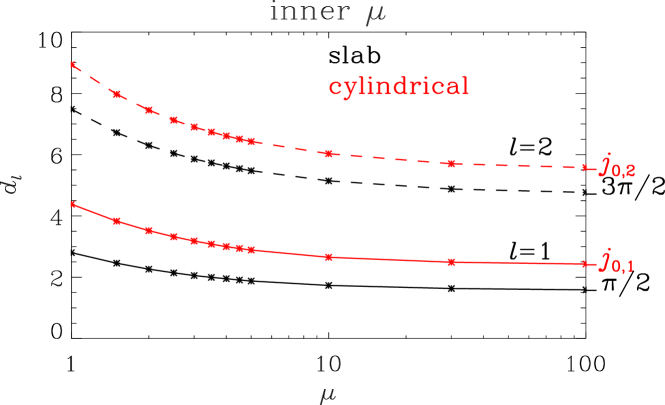
Figure 10: Similar to Figure 4 but for “inner $\mu$” profiles. Note that for this family of profiles, $f(x)$ conforms to $1-(x/R)^{\mu_{0}}$ when $x/R\ll 1$ and $(x/R)^{-\mu_{\infty}}$ when $x/R\gg 1$, with $\mu_{0}=\mu$ and $\mu_{\infty}=\infty$.

Figure 10 examines, in a format identical to Figure 4, how the dependence of $d_{l}$ on $\mu$ differs in the slab (the black curves) from the cylindrical geometry (red). One sees that the behavior of $d_{l}$ is distinct from what happens for the “$\mu$ power” and “outer $\mu$” profiles in two aspects. First, $d_{l}$ is always nonzero regardless of $\mu$ (or equivalently $\mu_{0}$). Second, while $d_{l}$ tends to increase with $\mu$ for the “$\mu$ power” and “outer $\mu$” profiles, it decreases with $\mu$ for the “inner $\mu$” profile in both geometries. This means that the profile details can substantially influence the cutoff wavenumbers, even though whether cutoff wavenumbers exist is entirely determined by the profile steepness far from the structure axis. Despite these two aspects, one sees once again that $d_{l}$ is always larger in the cylindrical case.

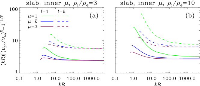
Figure 11: Similar to Figure 5 but for “inner $\mu$” profiles. Here $\beta=2\mu/(\mu+2)$. Note that for this family of profiles, $f(x)$ conforms to $1-(x/R)^{\mu_{0}}$ when $x/R\ll 1$ and $(x/R)^{-\mu_{\infty}}$ when $x/R\gg 1$, with $\mu_{0}=\mu$ and $\mu_{\infty}=\infty$.

Do Equations (32) to (34) also hold for trapped sausage waves in coronal slabs with the “inner $\mu$” profile? To examine this, Figure 11 shows the dependence on $kR$ of $(kR)[(v_{\rm ph}/v_{\rm Ai})^{2}-1]^{1/\beta}$ in a format identical to Figures 5 and 9. Here $\beta$ is given by Equation (33) in which we take $\mu_{0}=\mu$. Comparing any curve with its counterpart computed for the “$\mu$ power” profile, one sees that both curves attain the same asymptotic value, or equivalently $c_{l}$, despite that the curves show some evident difference when $kR$ is not that large. In fact, repeating the procedures involved in constructing Figures 6 and 7, we find exactly the same curves. The same can be said for the cylindrical case. On the one hand, this demonstrates that Equations (32) to (34) do hold for this family of profiles, and for coronal slabs and tubes alike. On the other hand, this lends further support to Conjecture 1 in that the steepness of $f(x)$ at the structure axis is the only factor that determines $h_{l}$.

8 SUMMARY AND CONCLUDING REMARKS

This study continues our study (Yu et al. 2017, paper I) on impulsively generated sausage wave trains in pressureless coronal structures, paying special attention to the effects of the transverse density distribution. While a cylindrical geometry was examined therein, this study focuses on a slab geometry to capitalize on its mathematical simplicity. A rather comprehensive survey of representative transverse density profiles was conducted, and the temporal and wavelet signatures of impulsively generated wave trains were examined in the context of the frequency $\omega$ (or equivalently the axial wavenumber $k$) dependence of the axial group speeds ($v_{\rm gr}$) of trapped modes. We have also examined the differences that a slab geometry introduces relative to the cylindrical results. Our results can be summarized as follows.

With the much-studied top-hat profile as an example, we showed that the temporal evolution and Morlet spectra computed for impulsively generated sausage wave trains in coronal slabs are remarkably similar to their cylindrical counterparts. In fact, they are similar to such an extent that it suffices to refer the readers to the cylindrical results as summarized in Table 1. Common to both geometries, we find that the $v_{\rm gr}-k$ curves play an essential role in shaping the Morlet spectra. In particular, the morphology of the Morlet spectra crucially depends on whether the group speed curves posses cutoff wavenumbers and whether they are monotonical. The classical crazy tadpoles are exclusively associated with the group speed curves that possess wavenumber cutoffs ($k_{{\rm c},l}$) and are nonmonotonical. However, the Morlet spectra in the initial stage in the wave trains are broadened by the appearance of “fins” associated with higher-order transverse harmonics when the group speed curves do not possess wavenumber cutoffs. Likewise, the Morlet spectra in the late stage tend not to have a broad head when the group speed curves are monotonical.

We went on to conduct a rather thorough analytical treatment of trapped sausage modes in coronal slabs for a substantial number of density profiles. When possible, we provided the analytical expressions for the cutoff wavenumbers (if they exist), and the wavenumber dependence of axial phase speeds in the immediate vicinity of these cutoffs as well as at sufficiently large wavenumbers. These analytical results are summarized in Table 4 in a self-contained manner. A thorough numerical analysis of the trapped modes further shows that the density profiles have to fall off no less rapidly than $x^{-2}$ at large distances for cutoff wavenumbers to exist. On the other hand, the monotonicity of the $v_{\rm gr}-k$ curves depends critically on the asymptotic behavior of the axial phase speed $v_{\rm ph}$ at sufficiently large $k$, which in turn is entirely determined by the profile steepness right at the slab axis. This asymptotic behavior is quantified by Equations (32) to (34), which involve only the generic function $f(x)$ that characterizes the transition of the density profiles from the internal to ambient values. Provided that $f(x)$ is approximately $1-(x/R)^{\mu_{0}}$ when $x\ll R$, our results suggest that $v_{\rm gr}$ will eventually increase (decrease) with $k$ at large $k$ when $\mu_{0}>2$ ($\mu_{0}<2$). The end result is, the $v_{\rm gr}-k$ curves will be nonmonotonical when $\mu_{0}>2$, and tend to be monotical when $\mu_{0}<2$.

The differences between the two geometries are quantified by the behavior of two dimensionless parameters, $d_{l}$ and $h_{l}$, which do not depend on the density contrast. Closely related to cutoff wavenumbers, $d_{l}$ is always larger in the cylindrical case, meaning that coronal slabs can trap sausage waves with longer axial wavelengths. On the other hand, $h_{l}$ is involved in the asymptotic behavior of $v_{\rm ph}$ at large $k$, and is found to be also larger in the cylindrical case. As indicated by Equation (35), this means that $v_{\rm gr}$ approaches the internal Alfvén speed more rapidly at large $k$ for sausage waves in coronal tubes than for their counterparts in coronal slabs.

What will be the seismological implications of this rather extensive parameter study for both the slab and cylindrical geometries? Or to be more specific, what to make of the Morlet spectra that look drastically different from crazy tadpoles? It is worth emphasizing that high temporal resolution is necessary for these spectra to be observationally found in the first place. Even for the cases where no cutoff wavenumbers exist and therefore the Morlet spectra extend to substantially longer periods than for classical crazy tadpoles, the pertinent periods are at most an order-of-magnitude longer than the transverse Alfvén time (see Figure 5d in paper I). For typical coronal structures, this transverse Alfvén time evaluates to about one second. This makes it difficult to discern a proper Morlet spectrum with currently available EUV instruments, not to mention the detection of the differences in different types of the spectra. That said, let us stress that sub-second cadence is readily available in such radio instruments as NoRH (up to 0.1 sec at dual frequencies of 17 and 34 GHz, see Takano et al. 1997) and the Siberian Solar Radio Telescope (SSRT, 14 ms for one-dimensional imaging observations, see Grechnev et al. 2003). Furthermore, the solar corona has been imaged in both white light and the coronal green line with a cadence as high as 45 ms with the Solar Eclipse Corona Imaging System (SECIS, see Williams et al. 2001). It therefore seems possible to dig into the available high-cadence data to look for the Morlet spectra other than crazy tadpoles. From the results found in the present study, one will be allowed to say that the density profile is likely to be rather gradual in the ambient corona if some “fins” can be identified. If, on the other hand, no broad head can be seen, then the density profile close to the structure axis in question is likely to be rather steep. This latter aspect is perhaps the most important application of the results from our study, because it offers a possible means to detect the information on the sub-resolution structuring inside coronal structures.

Albeit rather comprehensive, the present study does not exhaust the possible effects on impulsively generated sausage wave trains in coronal structures with continuous transverse structuring even when these structures are simply modeled as field-aligned density enhancements. First, it is evidently impossible to exhaust all possible density descriptions. Second, in addition to the density profile, the spatial scale of the initial perturbation can be equally important in determining the signatures of the wave trains. As was theoretically shown by Oliver et al. (2015), while the transverse density distribution determines the mode structures, the details of the initial perturbations will determine how the energy contained therein is apportioned to different modes. And this energy partition then determines the relative importance of different modes in contributing to the temporal evolution of the wave trains. Pursuing this aspect will provide a more complete picture on impulsively generated wave trains, but is left for another study in this series of manuscripts.

APPENDIX

Appendix A CORONAL SLABS WITH EXPONENTIAL PROFILES

This section examines coronal slabs with transverse density distributions of the form

$$\displaystyle f(x)=\exp\left(-\frac{x}{R}\right)~{},$$ (A1)

which has been examined by ER88 (see Conwell 1973 and Love & Ghatak 1979 for analogous studies in the context of optical fibers). The solution to Equation (11) has the form

$$\tilde{\xi}\propto J_{2\bar{m}}(X)~{},$$ (A2)

where $X=2\sqrt{\bar{D}}{\rm e}^{-x/(2R)}$. The DR for trapped sausage modes is given simply by the requirement that $\tilde{\xi}(x=0)=0$, resulting in

$$J_{2\bar{m}}(2\sqrt{\bar{D}})=0~{}.$$ (A3)

The cutoff wavenumbers are then given by

$$\displaystyle k_{{\rm c},l}=\frac{j_{0,l}/2}{\sqrt{\rho_{\rm i}/\rho_{\rm e}-1}}~{},$$ (A4)

which follows from $\bar{m}=0$ and $\bar{D}=k^{2}R^{2}(\rho_{\rm i}/\rho_{\rm e}-1)$. The expressions for both the DR (A3) and cutoff wavenumbers (A4) have already been given by ER88. We will further examine the dispersive properties of sausage modes both in the immediate vicinity of cutoff wavenumbers and at large axial wavenumbers.

To show what happens when $k$ exceeds $k_{{\rm c},l}$ by only a small amount, we start by noting that Equations (20) to (22) remain valid. Let $\bar{D}_{{\rm c},l}$ denote the value that $\bar{D}$ attains at $k_{{\rm c},l}$, which evaluates to $\bar{n}_{{\rm c},l}^{2}$. It is straightforward to show that $\bar{D}\approx\bar{D}_{{\rm c},l}(1+2\delta_{\omega})$. Now expanding the DR (A3) by seeing the order and argument as being independent from each other, one finds that

$$\displaystyle\left(2\bar{m}\right)\left[\frac{\partial}{\partial\nu}J_{\nu}\left(2\sqrt{\bar{D}_{{\rm c},l}}\right)\right]_{\nu=2\bar{m}\rightarrow 0}+2\left(\sqrt{\bar{D}}-\sqrt{\bar{D}_{{\rm c},l}}\right)\left[\frac{\partial}{\partial Z}J_{0}\left(Z\right)\right]_{Z=2\sqrt{\bar{D}_{{\rm c},l}}}=0.$$ (A5)

Note that $\partial J_{\nu}/\partial\nu|_{\nu\rightarrow 0}=(\pi/2)Y_{0}$ and $\partial J_{0}(Z)/\partial Z=-J_{1}(Z)$ (see AS, chapter 9). Some algebra shows that $\delta_{\omega}$ is related to $\delta_{k}$ by an equation in the same form as Equation (23) with $\eta$ now given by $\eta=(2/\pi)[J_{1}(j_{0,l})/Y_{0}(j_{0,l})]$. Consequently, the approximate expressions for the phase and group speeds are still given by Equations (24) and (25), respectively.

When $kR\rightarrow\infty$, it is easy to see that $\chi\equiv\sqrt{\bar{D}}/\bar{m}\rightarrow 1^{+}$ despite that both $\bar{D}$ and $\bar{m}$ approach infinity. Now let $\zeta$ denote the solution to

$$\displaystyle\frac{2}{3}\left(-\zeta\right)^{3/2}=\sqrt{\chi^{2}-1}-{\rm arcsec}\chi~{}.$$ (A6)

The uniform asymptotic expansion for $\bar{m}\rightarrow\infty$ through real values indicates that $J_{2\bar{m}}(2\bar{m}\chi)$ is dominated by a term associated with ${\rm Ai}[(2\bar{m})^{2/3}\zeta]$ (see DLMF 2016, Equation 10.20.4). This means that asymptotically $\zeta=a_{l}(2\bar{m})^{-2/3}$ with $a_{l}$ being the zeros of Airy’s function ${\rm Ai}$. On the other hand, letting $\chi^{2}=1/(1-\delta)$ with $0<\delta\ll 1$, one finds from Equation (A6) that $\delta=-2^{2/3}\zeta$. With the definitions given by Equation (17), one then finds that $v_{\rm ph}^{2}/v_{\rm Ai}^{2}=1+(1-\rho_{\rm e}/\rho_{\rm i})\delta$. Putting all these results together, we finally find that the approximate expressions for $v_{\rm ph}$ and $v_{\rm gr}$ at large $kR$ agree exactly with Equations (43) and (44), respectively.

Appendix B CORONAL SLABS WITH SYMMETRIC EPSTEIN PROFILES

This section examines coronal slabs with transverse density distributions of the form

$$\displaystyle f(x)={\rm sech}^{2}\left(\frac{x}{R}\right)~{},$$ (B1)

which is the symmetric Epstein profile. While the DR for trapped sausage modes in this case can be found in e.g., Cooper et al. (2003), Macnamara & Roberts (2011), and Chen et al. (2014), we think a detailed derivation will be informative. Furthermore, we will derive the expressions for both the cutoff wavenumbers and the asymptotic behavior of the phase and group speeds for arbitrary transverse order $l$, which are not available to our knowledge.

An equation identical in form to Equation (11) was originally treated in Landau & Lifshitz (1965, page 73) in the context of quantum mechanics (see Love & Ghatak 1979 for an analogous study treating optical fibers). With the definitions

$$\displaystyle X=\tanh\left(x/R\right)~{},$$ (B2)

$$\nu=\sqrt{\bar{D}+\frac{1}{4}}-\frac{1}{2}~{},$$ (B3)

Equation (11) becomes

$$\displaystyle\frac{{\rm d}}{{\rm d}X}\left[\left(1-X^{2}\right)\frac{{\rm d}\tilde{\xi}}{{\rm d}X}\right]+\left[\nu\left(\nu+1\right)-\frac{\bar{m}^{2}}{1-X^{2}}\right]\tilde{\xi}=0~{},$$ (B4)

which is the associated Legendre equation. While Landau & Lifshitz (1965) went on to transform Equation (B4) into the hypergeometric equation, we find that it is slightly more convenient to stick to this present form for examining sausage waves. The solution to Equation (B4) can be expressed as

$$\tilde{\xi}\propto C_{1}P_{\nu}^{\bar{m}}(X)+C_{2}Q_{\nu}^{\bar{m}}(X)~{},$$

where $P_{\nu}^{\bar{m}}$ and $Q_{\nu}^{\bar{m}}$ are the associated Legendre functions (AS, Chapter 8). For $\tilde{\xi}$ to vanish at $x\rightarrow\infty$ (and hence $X=1^{-}$), the two constants $C_{1}$ and $C_{2}$ need to be related by $C_{1}=-(C_{2}/2)\pi\cot(\bar{m}\pi)$. Evaluating $\tilde{\xi}$ at $x=0$ (and hence $X=0$) yields that

$$\displaystyle\tilde{\xi}(X=0)=-C_{2}\pi^{3/2}\frac{{\rm csc}(\bar{m}\pi)\Gamma(\bar{m}+\nu+1)}{\Gamma[(\bar{m}-\nu+1)/2]\Gamma(\nu-\bar{m}+1)\Gamma[(\bar{m}+\nu)/2+1]}~{},$$ (B5)

where $\Gamma$ is the Gamma function. Given that $\tilde{\xi}(X=0)=0$ for sausage modes, $\Gamma[(\bar{m}-\nu+1)/2]$ needs to diverge, meaning that $(\bar{m}-\nu+1)/2=0,-1,-2,\cdots$. In other words, the desired DR reads

$$\displaystyle\sqrt{\bar{D}+\frac{1}{4}}=\bar{m}+\left(2l-\frac{1}{2}\right)~{},$$ (B6)

with $l=1,2,3,\cdots$ being the transverse order. We note by passing that with $C_{1}$ and $C_{2}$ related in the above-mentioned manner, $\tilde{\xi}$ can be transformed into

$$\displaystyle\tilde{\xi}\propto\left(1-X^{2}\right)^{\bar{m}/2}F\left(\bar{m}+\nu+1,\bar{m}-\nu;\bar{m}+1;\frac{1-X}{2}\right)~{},$$ (B7)

where $F(a,b;c;\cdot)$ denotes the hypergeometric function $\,{}_{2}F_{1}$. Equation (B7) is identical to Equation (10) in Macnamara & Roberts (2011).

Solving Equation (B6) for $\omega^{2}$ can make the dependence of $\omega$ on $k$ more apparent. To this end, we first take the squares of both sides, resulting in

$$\displaystyle\bar{n}^{2}-2l(2l-1)=(4l-1)\bar{m}~{}.$$ (B8)

It then follows that

$$\frac{\omega^{2}R^{2}}{v_{\rm Ai}^{2}}$$ (B9)

$$= \left(kR\right)^{2}+\frac{4l(2l-1)-(4l-1)^{2}\rho_{\rm e}/\rho_{\rm i}}{2}$$

$$+ \frac{(4l-1)\sqrt{4(1-\rho_{\rm e}/\rho_{\rm i})(kR)^{2}+[(4l-1)^{2}(\rho_{\rm e}/\rho_{\rm i})^{2}-8l(2l-1)\rho_{\rm e}/\rho_{\rm i}]}}{2}~{}.$$

Furthermore, evaluating Equation (B6) at the cutoff ($v_{\rm ph}=v_{\rm Ae}$ and hence $\bar{m}=0$) yields a compact expression for the cutoff wavenumbers

$$\displaystyle k_{{\rm c},l}R=\frac{\sqrt{2l(2l-1)}}{\sqrt{\rho_{\rm i}/\rho_{\rm e}-1}}~{}.$$ (B10)

We note that the term in the square root on the RHS of Equation (B9) can be positive even when $k$ is smaller than $k_{{\rm c},l}$. However, the solution in the portion $k<k_{{\rm c},l}$ is spurious: plugging it in the LHS of Equation (B8) yields a negative value. This is not acceptable because with $\bar{m}$ (and $m$) negative, Equation (B7) indicates that the Lagrangian displacement $\tilde{\xi}$ becomes unbounded with distance, given that $X\rightarrow 1^{-}$ and $F[\cdot,\cdot;\cdot;(1-X)/2]\rightarrow 1$ when $x\rightarrow\infty$.

Approximate expressions for both $v_{\rm ph}$ and $v_{\rm gr}$ can be found when $k$ is larger than $k_{{\rm c},l}$ only marginally. The derivation is simpler than for top-hat and exponential profiles because we can now directly plug into Equation (B8) the definitions in Equations (20) to (22). One finds that $\delta_{\omega}$ is related to $\delta_{k}$ by an equation in the same form as Equation (23) with $\eta$ now given by $\eta=2\sqrt{2l(2l-1)}/(4l-1)$. The approximate behavior of the phase and group speeds can still be described by Equations (24) and (25), respectively.

We now look for the asymptotic behavior of the axial phase and group speeds at large axial wavenumbers. Starting with Equation (B9), we find that when $kR\rightarrow\infty$,

$$\displaystyle\frac{v_{\rm ph}}{v_{\rm Ai}} \approx 1+\frac{(2l-1/2)\sqrt{1-\rho_{\rm e}/\rho_{\rm i}}}{kR}-\frac{(2l-1/2)^{2}(1+\rho_{\rm e}/\rho_{\rm i})/2-l(2l-1)}{k^{2}R^{2}}~{},$$ (B11)

$$\frac{v_{\rm gr}}{v_{\rm Ai}} \approx 1+\frac{(2l-1/2)^{2}(1+\rho_{\rm e}/\rho_{\rm i})/2-l(2l-1)}{k^{2}R^{2}}~{}.$$ (B12)

One sees that Equations (B11) and (B12) agree with Equations (60) and (61), if the terms of order $1/(kR)^{2}$ are neglected. However, it can be readily shown that the numerator in the second term on the RHS of Equation (B12) is positive for arbitrary $\rho_{\rm e}/\rho_{\rm i}$. This means that eventually $v_{\rm gr}$ approaches $v_{\rm Ai}$ from above, which is opposite to what happens in the inner $\mu$ case with $\mu=2$.

Appendix C CORONAL SLABS WITH $f(x)=1/(1+x/R)^{2}$

This section examines coronal slabs with transverse density distributions of the form

$$\displaystyle f(x)=\frac{1}{(1+x/R)^{2}}~{},$$ (C1)

which has already been examined by LN15 (see Love & Ghatak 1979 for an analogous study treating optical fibers). The solution to Equation (11) is in the form

$$\displaystyle\tilde{\xi}\propto X^{1/2}K_{\nu}(X)~{},$$ (C2)

where

$$\displaystyle X=\bar{m}(1+x/R)~{},~{}~{}~{}\nu^{2}=\frac{1}{4}-\bar{D}~{}.$$ (C3)

The DR for trapped sausage modes simply follows from the requirement that $\tilde{\xi}(x=0)=0$, resulting in

$$\displaystyle K_{\nu}(\bar{m})=0~{}.$$ (C4)

Note that at large distances this profile reads $f(x)\approx R^{2}/x^{2}$, which is identical to our “$\mu$ power” case with $\mu=2$. Similar to the discussions therein, the cutoff wavenumbers should be still given by Equation (31), and $\nu$ is either zero or purely imaginary ($\nu^{2}\leq 0$).

The results up to this point have already been found by LN15. Therefore let us now offer some new analytical results by examining what happens when $kR\rightarrow\infty$. Note that in this case both $\bar{m}$ and $|\nu|$ approach infinity, but $\chi\equiv\bar{m}/|\nu|\rightarrow 1^{-}$. Using the asymptotic expansion for the modified Bessel function of purely imaginary order (see Olver 1997, page 425, Ex. 10.6), we find that $K_{i|\nu|}(|\nu|\chi)$ is dominated by a term proportional to ${\rm Ai}(-|\nu|^{2/3}\zeta)$, where $\zeta$ is the solution to

$$\displaystyle\frac{2}{3}\zeta^{3/2}=\ln\frac{1+(1-\chi^{2}){1/2}}{\chi}-(1-\chi^{2})^{1/2}~{}.$$ (C5)

This means that asymptotically $\zeta\approx(-a_{l})|\nu|^{-2/3}$. Now let $\chi^{2}=1-\delta$ with $0<\delta\ll 1$. Taylor expanding Equation (C5) to terms of order $\delta^{3/2}$, one finds that $\delta=2^{2/3}\zeta$. In addition, it is simple to show that $v_{\rm ph}^{2}/v_{\rm Ai}^{2}=1+\delta(1-\rho_{\rm e}/\rho_{\rm i})$, meaning that

$$\displaystyle\frac{v_{\rm ph}^{2}}{v_{\rm Ai}^{2}} \approx 1+(-a_{l})2^{2/3}(1-\rho_{\rm e}/\rho_{\rm i})(kR\sqrt{1-\rho_{\rm e}/\rho_{\rm i}})^{-2/3}$$ (C6)

$$\approx 1+\left[\frac{3\left(4l-1\right)\pi(1-\rho_{\rm e}/\rho_{\rm i})}{4kR}\right]^{2/3}~{},$$

where the second approximation follows from the accurate approximation to $a_{l}$, the $l$-th zero of Airy’s function ${\rm Ai}$ (see Equation 41). Consequently, the axial group speed at large $kR$ is given by

$$\displaystyle\frac{v_{\rm gr}^{2}}{v_{\rm Ai}^{2}}\approx 1+\frac{1}{3}\left[\frac{3\left(4l-1\right)\pi(1-\rho_{\rm e}/\rho_{\rm i})}{4kR}\right]^{2/3}~{}.$$ (C7)

This means that both $v_{\rm ph}$ and $v_{\rm gr}$ eventually approach $v_{\rm Ai}$ from above when $kR$ increases.

Table 1: Impulsively generated sausage wave trains in coronal slabs

profile	$f(x)$ at $x/R\ll 1$	$f(x)$ at $x/R\gg 1$	$[\mu_{0},\mu_{\infty}]$	Group Speed Curves	Morlet Spectra
$\mu$ power	$\approx 1-(x/R)^{\mu}$	$\approx(x/R)^{-\mu}$	$[\mu,\mu]$	See Fig. 4 in paper I	See Figs. 5 & 6 in paper I
outer $\mu$	$=1$	$=(x/R)^{-\mu}$	$[\infty,\mu]$	See Fig. 7 in paper I	See Figs. 8 & 9 in paper I
inner $\mu$	$=1-(x/R)^{\mu}$	$=0$	$[\mu,\infty]$	See Figs. 10 & 11 in paper I	See Figs. 12 & 13 in paper I

Table 2: Comparison of $d_{l}$ between the slab and cylindrical geometries

$f(x)$	$l$	Slab	Cylindrical
top-hat	$l=1$	$\pi/2=1.57$	$j_{0,1}=2.41$
	$l=2$	$3\pi/2=4.71$	$j_{0,2}=5.52$
	$l=3$	$5\pi/2=7.85$	$j_{0,3}=8.65$
$1/(1+x/R)^{2}$	arbitrary $l$	$1/2$	$1$
$\exp(-x/R)$	$l=1$	$j_{0,1}/2=1.20$	$1.95$
	$l=2$	$j_{0,2}/2=2.76$	$3.44$
(see note c)	$l=3$	$j_{0,3}/2=4.33$	$4.97$
${\rm sech}^{2}(x/R)$	$l=1$	$1.41$	$2.26$
	$l=2$	$3.46$	$4.23$
(see note d)	$l=3$	$5.48$	$6.21$

Table 3: Comparison of $h_{l}$ between the slab and cylindrical geometries

$f(x)$	$f(x)$ at small $x/R$	$l$	Slab	Cylindrical
top-hat	$1-(x/R)^{\infty}$	$l=1$	$\pi=3.14$	$j_{1,1}=3.83$
		$l=2$	$2\pi=6.28$	$j_{1,2}=7.02$
$\exp(-x/R)$	$\approx 1-(x/R)$	$l=1$	$3.53$	$4.89$
(see note c)		$l=2$	$8.25$	$9.62$
${\rm sech}^{2}(x/R)$	$\approx 1-(x/R)^{2}$	$l=1$	$3$	$4$
(see note d)		$l=2$	$7$	$8$

Table 4: Summary of analytical behavior of trapped sausage modes in coronal slabs

profile	$f(x)$	Dispersion Relation	$d_{l}$ in cutoff	($c_{l},\beta$) in $v_{\rm ph}$ at	References
			wavenumbers	large wavenumbers
top-hat	$1$ if $x\leq R$	$\bar{n}\cot\bar{n}=-\bar{m}$	$(l-1/2)\pi$	$c_{l}=l\pi$	ER82, also Sect. 3.1
	$0$ if $x>R$			$\beta=2$
$\mu$ power	$\displaystyle\frac{1}{1+x/R}$	$W_{\nu,1/2}(2\bar{m})=0$	no cutoff	$\displaystyle c_{l}=\frac{3(4l-1)\pi(1-\rho_{\rm e}/\rho_{\rm i})}{8}$	LN15, also Sect. 5.1
($\mu=1$)
		where $\nu=\bar{D}/(2\bar{m})$		$\beta=2/3$
outer $\mu$	$1$ if $x\leq R$	$\displaystyle\bar{n}\cot\bar{n}=\bar{m}-\nu-\frac{W_{\nu+1,1/2}(2\bar{m})}{W_{\nu,1/2}(2\bar{m})}$	no cutoff	$c_{l}=l\pi$	Sect. 6.1
($\mu=1$)	$(x/R)^{-1}$
	if $x>R$	where $\nu=\bar{D}/(2\bar{m})$		$\beta=2$
outer $\mu$	$1$ if $x\leq R$	$\displaystyle\bar{n}\cot\bar{n}=\frac{1}{2}-\nu-\bar{m}\frac{K_{\nu-1}(\bar{m})}{K_{\nu}(\bar{m})}$	$\displaystyle\frac{1}{2}$	$c_{l}=l\pi$	Sect. 6.1
($\mu=2$)	$(x/R)^{-2}$
	if $x>R$	where $\nu^{2}=1/4-\bar{D}$		$\beta=2$
inner $\mu$	$1-x/R$	$\frac{{\rm Bi}(X_{0}){\rm Ai}^{\prime}(X_{1})-{\rm Ai}(X_{0}){\rm Bi}^{\prime}(X_{1})}{{\rm Bi}(X_{0}){\rm Ai}(X_{1})-{\rm Ai}(X_{0}){\rm Bi}(X_{1})}=-\frac{\bar{m}}{\bar{D}^{1/3}}$	$\approx\displaystyle\frac{3\pi}{2}\left(l-\frac{5}{12}\right)$	$c_{l}=\displaystyle\frac{3(4l-1)\pi(1-\rho_{\rm e}/\rho_{\rm i})}{8}$	Sect. 7.1
($\mu=1$)	if $x\leq R$
	$0$ if $x>R$	where $X_{0}=-\bar{n}^{2}/\bar{D}^{2/3},X_{1}=\bar{m}^{2}/\bar{D}^{2/3}$		$\beta=2/3$
inner $\mu$	$1-x^{2}/R^{2}$	$\displaystyle-\bar{m}=1-p+\frac{4p(\alpha+1/2)}{3}\frac{M(\alpha+3/2,5/2,p)}{M(\alpha+1/2,3/2,p)}$	$\approx 4l-1$	$c_{l}=(4l-1)\sqrt{1-\rho_{\rm e}/\rho_{\rm i}}$	ER88, also Sect. 7.1
($\mu=2$)	if $x\leq R$
	$0$ if $x>R$	where $p=\bar{D}^{1/2},\alpha=1/4-\bar{n}^{2}/(4p)$		$\beta=1$
exponential	$\exp(-x/R)$	$J_{2\bar{m}}(2\sqrt{\bar{D}})=0$	$j_{0,l}/2$	$c_{l}=\displaystyle\frac{3(4l-1)\pi(1-\rho_{\rm e}/\rho_{\rm i})}{8}$	ER88 (C73, LG79),
				$\beta=2/3$	also Appendix A
Epstein	${\rm sech}^{2}(x/R)$	$\displaystyle\sqrt{\bar{D}+\frac{1}{4}}=\bar{m}+2l-\frac{1}{2}$	$\sqrt{2l(2l-1)}$	$c_{l}=(4l-1)\sqrt{1-\rho_{\rm e}/\rho_{\rm i}}$	ER88, CNW03, MR11
				$\beta=1$	(LL65, LG79), also Appendix B
	$\displaystyle\frac{1}{(1+x/R)^{2}}$	$K_{\nu}(\bar{m})=0$	$\displaystyle\frac{1}{2}$	$\displaystyle c_{l}=\frac{3(4l-1)\pi(1-\rho_{\rm e}/\rho_{\rm i})}{4}$	LN15 (LG79)
		where $\nu^{2}=1/4-\bar{D}$		$\beta=2/3$	also Appendix C

Figure 2: Dependence on the axial wavenumber $k$ of the axial phase (the upper row) and group (lower) speeds for top-hat profiles with a density contrast of $3$ (the left column) and $10$ (right). The solid (dashed) curves represent the first (second) branch of trapped modes, corresponding to a transverse order of $1$ ($2$). The horizontal dash-dotted lines represent the internal and external Alfvén speeds ($v_{\rm Ai}$ and $v_{\rm Ae}$). Note that in the lower row, the horizontal line representing $v_{\rm Ae}$ is absent because $v_{\rm Ae}$ is beyond the range of the vertical axis.

References

- Abramowitz & Stegun (1972) Abramowitz, M. & Stegun, I. A. 1972, Handbook of Mathematical Functions
- Arregui (2015) Arregui, I. 2015, Philosophical Transactions of the Royal Society of London Series A, 373, 20140261
- Arregui et al. (2007a) Arregui, I., Andries, J., Van Doorsselaere, T., Goossens, M., & Poedts, S. 2007a, A&A, 463, 333
- Arregui & Asensio Ramos (2014) Arregui, I. & Asensio Ramos, A. 2014, A&A, 565, A78
- Arregui et al. (2012) Arregui, I., Oliver, R., & Ballester, J. L. 2012, Living Reviews in Solar Physics, 9, 2
- Arregui et al. (2007b) Arregui, I., Terradas, J., Oliver, R., & Ballester, J. L. 2007b, Sol. Phys., 246, 213
- Aschwanden et al. (1999) Aschwanden, M. J., Fletcher, L., Schrijver, C. J., & Alexander, D. 1999, ApJ, 520, 880
- Aschwanden et al. (2004) Aschwanden, M. J., Nakariakov, V. M., & Melnikov, V. F. 2004, ApJ, 600, 458
- Aschwanden & Schrijver (2011) Aschwanden, M. J. & Schrijver, C. J. 2011, ApJ, 736, 102
- Ballai (2007) Ballai, I. 2007, Sol. Phys., 246, 177
- Banerjee et al. (2007) Banerjee, D., Erdélyi, R., Oliver, R., & O’Shea, E. 2007, Sol. Phys., 246, 3
- Cally (1986) Cally, P. S. 1986, Sol. Phys., 103, 277
- Cargill (2009) Cargill, P. J. 2009, Space Sci. Rev., 144, 413
- Chen (2016) Chen, P. F. 2016, Washington DC American Geophysical Union Geophysical Monograph Series, 216, 381
- Chen et al. (2014) Chen, S.-X., Li, B., Xia, L.-D., Chen, Y.-J., & Yu, H. 2014, Sol. Phys., 289, 1663
- Chen et al. (2015a) Chen, S.-X., Li, B., Xia, L.-D., & Yu, H. 2015a, Sol. Phys., 290, 2231
- Chen et al. (2015b) Chen, S.-X., Li, B., Xiong, M., Yu, H., & Guo, M.-Z. 2015b, ApJ, 812, 22
- Chen et al. (2016) —. 2016, ApJ, 833, 114
- Chen et al. (2011) Chen, Y., Feng, S. W., Li, B., Song, H. Q., Xia, L. D., Kong, X. L., & Li, X. 2011, ApJ, 728, 147
- Chen et al. (2010) Chen, Y., Song, H. Q., Li, B., Xia, L. D., Wu, Z., Fu, H., & Li, X. 2010, ApJ, 714, 644
- Conwell (1973) Conwell, E. M. 1973, Applied Physics Letters, 23, 328
- Cooper et al. (2003) Cooper, F. C., Nakariakov, V. M., & Williams, D. R. 2003, A&A, 409, 325
- De Moortel & Browning (2015) De Moortel, I. & Browning, P. 2015, Philosophical Transactions of the Royal Society of London Series A, 373, 20140269
- De Moortel & Nakariakov (2012) De Moortel, I. & Nakariakov, V. M. 2012, Philosophical Transactions of the Royal Society of London Series A, 370, 3193
- De Pontieu et al. (2007) De Pontieu, B., McIntosh, S. W., Carlsson, M., Hansteen, V. H., Tarbell, T. D., Schrijver, C. J., Title, A. M., Shine, R. A., Tsuneta, S., Katsukawa, Y., Ichimoto, K., Suematsu, Y., Shimizu, T., & Nagata, S. 2007, Science, 318, 1574
- DLMF (2016) DLMF. 2016, NIST Digital Library of Mathematical Functions, http://dlmf.nist.gov/, Release 1.0.13 of 2016-09-16, f. W. J. Olver, A. B. Olde Daalhuis, D. W. Lozier, B. I. Schneider, R. F. Boisvert, C. W. Clark, B. R. Miller and B. V. Saunders, eds.
- Dorotovič et al. (2014) Dorotovič, I., Erdélyi, R., Freij, N., Karlovský, V., & Márquez, I. 2014, A&A, 563, A12
- Dorotovič et al. (2008) Dorotovič, I., Erdélyi, R., & Karlovský, V. 2008, in IAU Symposium, Vol. 247, Waves & Oscillations in the Solar Atmosphere: Heating and Magneto-Seismology, ed. R. Erdélyi & C. A. Mendoza-Briceno, 351–354
- Edwin & Roberts (1982) Edwin, P. M. & Roberts, B. 1982, Sol. Phys., 76, 239
- Edwin & Roberts (1983) —. 1983, Sol. Phys., 88, 179
- Edwin & Roberts (1986) Edwin, P. M. & Roberts, B. 1986, in NASA Conference Publication, Vol. 2449, NASA Conference Publication, ed. B. R. Dennis, L. E. Orwig, & A. L. Kiplinger
- Edwin & Roberts (1988) —. 1988, A&A, 192, 343
- Erdélyi & Taroyan (2008) Erdélyi, R. & Taroyan, Y. 2008, A&A, 489, L49
- Freij et al. (2016) Freij, N., Dorotovič, I., Morton, R. J., Ruderman, M. S., Karlovský, V., & Erdélyi, R. 2016, ApJ, 817, 44
- Fu et al. (1990) Fu, Q.-J., Jin, S.-Z., Zhao, R.-Y., & Gong, Y.-F. 1990, Sol. Phys., 130, 161
- Goossens et al. (2002) Goossens, M., Andries, J., & Aschwanden, M. J. 2002, A&A, 394, L39
- Goossens et al. (2008) Goossens, M., Arregui, I., Ballester, J. L., & Wang, T. J. 2008, A&A, 484, 851
- Grant et al. (2015) Grant, S. D. T., Jess, D. B., Moreels, M. G., Morton, R. J., Christian, D. J., Giagkiozis, I., Verth, G., Fedun, V., Keys, P. H., Van Doorsselaere, T., & Erdélyi, R. 2015, ApJ, 806, 132
- Grechnev et al. (2003) Grechnev, V. V., Lesovoi, S. V., Smolkov, G. Y., Krissinel, B. B., Zandanov, V. G., Altyntsev, A. T., Kardapolova, N. N., Sergeev, R. Y., Uralov, A. M., Maksimov, V. P., & Lubyshev, B. I. 2003, Sol. Phys., 216, 239
- Guo et al. (2016) Guo, M.-Z., Chen, S.-X., Li, B., Xia, L.-D., & Yu, H. 2016, Sol. Phys., 291, 877
- He et al. (2009) He, J., Marsch, E., Tu, C., & Tian, H. 2009, ApJ, 705, L217
- Heyvaerts & Priest (1983) Heyvaerts, J. & Priest, E. R. 1983, A&A, 117, 220
- Hollweg & Yang (1988) Hollweg, J. V. & Yang, G. 1988, J. Geophys. Res., 93, 5423
- Hornsey et al. (2014) Hornsey, C., Nakariakov, V. M., & Fludra, A. 2014, A&A, 567, A24
- Jelínek & Karlický (2012) Jelínek, P. & Karlický, M. 2012, A&A, 537, A46
- Jess et al. (2009) Jess, D. B., Mathioudakis, M., Erdélyi, R., Crockett, P. J., Keenan, F. P., & Christian, D. J. 2009, Science, 323, 1582
- Karlický et al. (2013) Karlický, M., Mészárosová, H., & Jelínek, P. 2013, A&A, 550, A1
- Katsiyannis et al. (2003) Katsiyannis, A. C., Williams, D. R., McAteer, R. T. J., Gallagher, P. T., Keenan, F. P., & Murtagh, F. 2003, A&A, 406, 709
- Kitzhofer et al. (2009) Kitzhofer, G., Koch, O., & Weinmüller, E. 2009, in American Institute of Physics Conference Series, Vol. 1168, American Institute of Physics Conference Series, ed. T. E. Simos, G. Psihoyios, & C. Tsitouras, 39–42
- Klimchuk (2006) Klimchuk, J. A. 2006, Sol. Phys., 234, 41
- Kolotkov et al. (2015) Kolotkov, D. Y., Nakariakov, V. M., Kupriyanova, E. G., Ratcliffe, H., & Shibasaki, K. 2015, A&A, 574, A53
- Kopylova et al. (2007) Kopylova, Y. G., Melnikov, A. V., Stepanov, A. V., Tsap, Y. T., & Goldvarg, T. B. 2007, Astronomy Letters, 33, 706
- Landau & Lifshitz (1965) Landau, L. D. & Lifshitz, E. M. 1965, Quantum mechanics
- Li et al. (2014) Li, B., Chen, S.-X., Xia, L.-D., & Yu, H. 2014, A&A, 568, A31
- Li et al. (2013) Li, B., Habbal, S. R., & Chen, Y. 2013, ApJ, 767, 169
- Liu & Ofman (2014) Liu, W. & Ofman, L. 2014, Sol. Phys., 289, 3233
- Lopin & Nagorny (2015a) Lopin, I. & Nagorny, I. 2015a, ApJ, 801, 23
- Lopin & Nagorny (2015b) —. 2015b, ApJ, 810, 87
- Love & Ghatak (1979) Love, J. D. & Ghatak, A. K. 1979, IEEE Journal of Quantum Electronics, 15, 14
- Macnamara & Roberts (2011) Macnamara, C. K. & Roberts, B. 2011, A&A, 526, A75
- Mészárosová et al. (2011) Mészárosová, H., Karlický, M., & Rybák, J. 2011, Sol. Phys., 273, 393
- Mészárosová et al. (2009) Mészárosová, H., Karlický, M., Rybák, J., & Jiřička, K. 2009, A&A, 502, L13
- Morton et al. (2011) Morton, R. J., Erdélyi, R., Jess, D. B., & Mathioudakis, M. 2011, ApJ, 729, L18
- Morton et al. (2012) Morton, R. J., Verth, G., Jess, D. B., Kuridze, D., Ruderman, M. S., Mathioudakis, M., & Erdélyi, R. 2012, Nature Communications, 3, 1315
- Murawski & Roberts (1993) Murawski, K. & Roberts, B. 1993, Sol. Phys., 144, 101
- Murawski & Roberts (1994) —. 1994, Sol. Phys., 151, 305
- Nakariakov et al. (2004) Nakariakov, V. M., Arber, T. D., Ault, C. E., Katsiyannis, A. C., Williams, D. R., & Keenan, F. P. 2004, MNRAS, 349, 705
- Nakariakov et al. (2012) Nakariakov, V. M., Hornsey, C., & Melnikov, V. F. 2012, ApJ, 761, 134
- Nakariakov & Melnikov (2009) Nakariakov, V. M. & Melnikov, V. F. 2009, Space Sci. Rev., 149, 119
- Nakariakov et al. (1999) Nakariakov, V. M., Ofman, L., Deluca, E. E., Roberts, B., & Davila, J. M. 1999, Science, 285, 862
- Nakariakov et al. (2016) Nakariakov, V. M., Pilipenko, V., Heilig, B., Jelínek, P., Karlický, M., Klimushkin, D. Y., Kolotkov, D. Y., Lee, D.-H., Nisticò, G., Van Doorsselaere, T., Verth, G., & Zimovets, I. V. 2016, Space Sci. Rev., 200, 75
- Nakariakov & Verwichte (2005) Nakariakov, V. M. & Verwichte, E. 2005, Living Reviews in Solar Physics, 2, 3
- Ofman & Wang (2008) Ofman, L. & Wang, T. J. 2008, A&A, 482, L9
- Oliver et al. (2015) Oliver, R., Ruderman, M. S., & Terradas, J. 2015, ApJ, 806, 56
- Olver (1997) Olver, F. 1997, Asymptotics and Special Functions
- Parnell & De Moortel (2012) Parnell, C. E. & De Moortel, I. 2012, Philosophical Transactions of the Royal Society of London Series A, 370, 3217
- Pasachoff & Ladd (1987) Pasachoff, J. M. & Ladd, E. F. 1987, Sol. Phys., 109, 365
- Pasachoff & Landman (1984) Pasachoff, J. M. & Landman, D. A. 1984, Sol. Phys., 90, 325
- Pneuman (1965) Pneuman, G. W. 1965, Physics of Fluids, 8, 507
- Roberts (2000) Roberts, B. 2000, Sol. Phys., 193, 139
- Roberts (2008) Roberts, B. 2008, in IAU Symposium, Vol. 247, Waves & Oscillations in the Solar Atmosphere: Heating and Magneto-Seismology, ed. R. Erdélyi & C. A. Mendoza-Briceno, 3–19
- Roberts et al. (1983) Roberts, B., Edwin, P. M., & Benz, A. O. 1983, Nature, 305, 688
- Roberts et al. (1984) —. 1984, ApJ, 279, 857
- Rosenberg (1970) Rosenberg, H. 1970, A&A, 9, 159
- Ruderman & Roberts (2002) Ruderman, M. S. & Roberts, B. 2002, ApJ, 577, 475
- Samanta et al. (2016) Samanta, T., Singh, J., Sindhuja, G., & Banerjee, D. 2016, Sol. Phys., 291, 155
- Selwa et al. (2004) Selwa, M., Murawski, K., & Kowal, G. 2004, A&A, 422, 1067
- Shestov et al. (2015) Shestov, S., Nakariakov, V. M., & Kuzin, S. 2015, ApJ, 814, 135
- Soler et al. (2014) Soler, R., Goossens, M., Terradas, J., & Oliver, R. 2014, ApJ, 781, 111
- Takano et al. (1997) Takano, T., Nakajima, H., Enome, S., Shibasaki, K., Nishio, M., Hanaoka, Y., Shiomi, Y., Sekiguchi, H., Kawashima, S., Bushimata, T., Shinohara, N., Torii, C., Fujiki, K., & Irimajiri, Y. 1997, in Lecture Notes in Physics, Berlin Springer Verlag, Vol. 483, Coronal Physics from Radio and Space Observations, ed. G. Trottet, 183
- Terradas et al. (2005) Terradas, J., Oliver, R., & Ballester, J. L. 2005, A&A, 441, 371
- Tian et al. (2014) Tian, H., DeLuca, E. E., Cranmer, S. R., De Pontieu, B., Peter, H., Martínez-Sykora, J., Golub, L., McKillop, S., Reeves, K. K., Miralles, M. P., McCauley, P., Saar, S., Testa, P., Weber, M., Murphy, N., Lemen, J., Title, A., Boerner, P., Hurlburt, N., Tarbell, T. D., Wuelser, J. P., Kleint, L., Kankelborg, C., Jaeggli, S., Carlsson, M., Hansteen, V., & McIntosh, S. W. 2014, Science, 346, 1255711
- Torrence & Compo (1998) Torrence, C. & Compo, G. P. 1998, Bulletin of the American Meteorological Society, 79, 61
- Uchida (1970) Uchida, Y. 1970, PASJ, 22, 341
- Van Doorsselaere et al. (2016) Van Doorsselaere, T., Kupriyanova, E. G., & Yuan, D. 2016, Sol. Phys., 291, 3143
- Verwichte et al. (2009) Verwichte, E., Aschwanden, M. J., Van Doorsselaere, T., Foullon, C., & Nakariakov, V. M. 2009, ApJ, 698, 397
- Verwichte et al. (2005) Verwichte, E., Nakariakov, V. M., & Cooper, F. C. 2005, A&A, 430, L65
- Wang (2016) Wang, T. J. 2016, Washington DC American Geophysical Union Geophysical Monograph Series, 216, 395
- Warmuth (2015) Warmuth, A. 2015, Living Reviews in Solar Physics, 12, 3
- Warmuth & Mann (2005) Warmuth, A. & Mann, G. 2005, A&A, 435, 1123
- White & Verwichte (2012) White, R. S. & Verwichte, E. 2012, A&A, 537, A49
- Wilhelm et al. (2011) Wilhelm, K., Abbo, L., Auchère, F., Barbey, N., Feng, L., Gabriel, A. H., Giordano, S., Imada, S., Llebaria, A., Matthaeus, W. H., Poletto, G., Raouafi, N.-E., Suess, S. T., Teriaca, L., & Wang, Y.-M. 2011, A&A Rev., 19
- Williams et al. (2002) Williams, D. R., Mathioudakis, M., Gallagher, P. T., Phillips, K. J. H., McAteer, R. T. J., Keenan, F. P., Rudawy, P., & Katsiyannis, A. C. 2002, MNRAS, 336, 747
- Williams et al. (2001) Williams, D. R., Phillips, K. J. H., Rudawy, P., Mathioudakis, M., Gallagher, P. T., O’Shea, E., Keenan, F. P., Read, P., & Rompolt, B. 2001, MNRAS, 326, 428
- Yu et al. (2016a) Yu, H., Li, B., Chen, S.-X., Xiong, M., & Guo, M.-Z. 2016a, ApJ, 833, 51
- Yu et al. (2017) —. 2017, ApJ, 836, 1
- Yu et al. (2016b) Yu, S., Nakariakov, V. M., & Yan, Y. 2016b, ApJ, 826, 78
- Zajtsev & Stepanov (1975) Zajtsev, V. V. & Stepanov, A. V. 1975, Issledovaniia Geomagnetizmu Aeronomii i Fizike Solntsa, 37, 3
- Zaqarashvili & Erdélyi (2009) Zaqarashvili, T. V. & Erdélyi, R. 2009, Space Sci. Rev., 149, 355