Solar Bayesian Analysis Toolkit — a new Markov chain Monte Carlo IDL code for Bayesian parameter inference

Abstract

We present the Solar Bayesian Analysis Toolkit (SoBAT) which is a new easy to use tool for Bayesian analysis of observational data, including parameter inference and model comparison. SoBAT is aimed (but not limited) to be used for the analysis of solar observational data. We describe a new Interactive Data Language (IDL) code designed to facilitate the comparison of user-supplied model with data. Bayesian inference allows prior information to be taken into account. The use of Markov chain Monte Carlo (MCMC) sampling allows efficient exploration of large parameter spaces and provides reliable estimation of model parameters and their uncertainties. The Bayesian evidence for different models can be used for quantitative comparison. The code is tested to demonstrate its ability to accurately recover a variety of parameter probability distributions. Its application to practical problems is demonstrated using studies of the structure and oscillation of coronal loops.

1 Introduction

The use of Bayesian analysis and Markov chain Monte Carlo (MCMC) sampling is increasingly common in astronomy (e.g. review by Sharma, 2017) and heliosesmology (e.g. Broomhall et al., 2010; Howe et al., 2015). However, it is not widely used in other branches of solar physics, with exception of magnetohydrodynamic (MHD) seismology of the solar corona, where the advantages of the Bayesian approach are intensively exploited. The details can be found in a recent review considering the use of Bayesian analysis for coronal seismology in particular (Arregui, 2018).

Traditionally, the problem of estimating model parameters from observational data (parameter inference) is solved by the best fitting approach which aims to find in the parameter space a point giving the best agreement between the model and observations. This is usually done by computing the maximum likelihood estimate (MLE) or least squares estimate (LSE) which is equal to MLE in the case of the normally distributed measurement errors. Thus, the aim of the best fitting approach is to find in the parameter space the global maximum corresponding to the best fit of the model to the observed data. The Bayesian approach is different: instead of searching for the highest peak in the parameter space, it implies making a map of the whole parameter space in the form of posterior probability distribution function (PDF) representing all information available from both observations and prior knowledge. This function gives a probability density for every point in the parameter space reaching a global maximum at the position corresponding to the best fitting combination of model parameters.

This lead us to the main advantage of the Bayesian approach which is a correct estimation of the uncertainties. Although, least squares fitting software often provides uncertainties estimation based on some assumptions like the Gaussian shape of a parameter distribution, such an estimation became incorrect when these assumptions are not valid, for example, if the parameter distribution significantly differs from the normal one (e.g. asymmetric or multi-modal). Since the Bayesian analysis is capable to recover even a complex parameter distribution being very different from the normal one, it allows for correct and reliable estimation of the uncertainties for a broad range of parameter inference problems.

Often, there are more than one models that can explain observational data. In this case, one needs to have a possibility to quantitatively compare competing models. A good model should have the following properties:

1. The best fit produced by the model should be close to the observed data points.

2. The model should not be over-fitted by having too many free parameters.

3. It should be confined in the parameter space. The model parameters should be well constrained based on the observational data.

4. It should be confined in the observational data space. The model should not predict observations far away from the actual data points.

To assess a model within the traditional best fitting approach the reduced $\chi^{2}$ criterion is mainly used. Though it allows us to assess the best fits (point 1) and accounts for the number of model parameters (point 2), it does not take into account the last two items from the list above and ignores the model confinement in the parameter and data spaces. Opposite to this, the Bayesian analysis offer a model comparison criterion called Bayes factor that assesses the whole models but not only the best fits and transparently accounts for all four properties mentioned in the list above.

The advantage of the Bayesian approach could be illustrated by the following specific example. In coronal seismology, one of the standard operations is the determination of parameters of kink oscillations. Suppose the observations gives us a time series of the oscillating displacements of a coronal loop. Theory predicts that the oscillation could be damped by either exponential or Gaussian law, and that the oscillation could be a superposition of several harmonics. Thus, the observationally obtained time series could be approximated by several different theoretically prescribed functions. For each specific function, its parameters that best fit the data could be determined by the MLE or LSE. However, the Bayesian analysis allows us to compare the quality of fittings by those different functions with each other.

The aim of this work is to provide the solar physics community with a reliable and easy to use tool for Bayesian analysis of observational data, including parameter inference and model comparison. Although, there are few efforts to bring Bayesian methodology to the IDL community (see e.g. idl_emcee sampler at https://github.com/mcfit/idl_emcee), according to our knowledge our IDL code provides unique features such as high level routines for “fitting” observational data and numerical tools for Bayesian model comparison.

This paper is organised as follows; the Bayesian method and techniques used in the code are presented in Sect. 2. Tests of the sampling algorithm are performed in Sect. 4. The code is demonstrated by applying it to simple test problems in Sect. 5, and to practical solar physics problems in Sect. 6. Concluding remarks are presented in Sect. 7.

2 Bayesian approach to parameter inference

A parameter inference problem implies that the observed data $D$ can be explained in terms of the model $M$ (i.e. an analytical function such as a sinusoid, a Gaussian, or even an underlying numerical code) having a parameter set $\theta=[\theta_{1},\theta_{2},...,\theta_{n}]$. For example, in the case of a sinusoidal function, $\theta_{i}$ can be the values of the period, amplitude, and phase. Thus, the aim is to find the value of the parameters $\theta$ that gives the best possible agreement with the observed data $D$. The formulation of the Bayesian parameter inference relies on three main definitions:

1. The prior probability density function (PDF) $P(\theta)$ represents our knowledge about the model parameters $\theta$ before considering the observational data $D$. For example, this could be knowledge from previous measurements or a requirement that the particular model parameter lies inside a certain range.

2. The sampling PDF $P(D|\theta)$ describes the conditional probability to obtain the observed data $D$ given that the model parameters $\theta$ are fixed. The sampling PDF is closely related to the measurement errors. For example, if measurement errors in our experiment follow (or can be assumed to follow) the normal distribution, the sampling PDF would be a normalised Gaussian.

3. The likelihood function is literately the sampling PDF $P(D|\theta)$ considered as a function of $\theta$ with fixed $D$. We note that in contrast to the sampling PDF, the likelihood function is not a probability density. In particular, its integral over $\theta$ is not equal to unity. To become a posterior PDF, the likelihood function needs to be normalised.

4. The posterior PDF $P(\theta|D)$ describes the conditional probability that the model parameters are equal to $\theta$ under condition of observed data being equal to $D$. This function represents our knowledge on the model parameters $\theta$ after the observation, when the observed data $D$ is known and fixed.

The Bayes theorem connects prior and posterior probability density functions and describes how the observational data $D$ affects our knowledge about model parameters $\theta$

$$P(\theta|D)=\frac{P(D|\theta)P(\theta)}{P(D)}.$$ (1)

The normalisation constant $P(D)$ is the Bayesian Evidence or marginalised likelihood

$$P(D)=\int P(D|\theta)P(\theta)d\theta$$ (2)

For our prescribed prior probability $P(\theta)$ and likelihood $P(D|\theta)$ functions, the posterior probability distribution $P(\theta|D)$ can be readily computed for any value of the parameter set $\theta$ using the Bayes theorem in Eq. (1). However, in practical applications, we are interested in finding an estimate and corresponding uncertainties for each parameter $\theta_{i}$.

The most common choice in Bayesian statistics for an estimate of unknown parameters $\theta$ is a maximum a posteriori probability (MAP) estimate $\theta_{MAP}$ which is a point in the parameter space where the posterior PDF reaches its global maximum. Other estimates e.g. the expected value or the median can be also used.

To put uncertainties around the estimate, one needs to calculate the marginalised (integrated) posteriors

$$P(\theta_{i}|D)=\int P(\theta_{1},\theta_{2},...,\theta_{N}|D)d\theta_{k\neq i}.$$ (3)

For a simple low-parametric model (2–3 parameters), the multiple integrals in Eq. (3) can be directly calculated using standard numerical methods. Unfortunately, it is practically impossible to use direct numerical integration for complicated models with a large set of parameters. Indeed, every additional parameter increases the computation time by several orders of magnitude. Therefore, sampling methods based on MCMC are preferable for complex models. MCMC allows us to obtain samples from the posterior probability distribution $P(\theta|D)$. When enough samples are obtained, the marginalised posterior (Eq. (3)) can be approximated by a histogram of the corresponding model parameter $\theta_{i}$.

2.1 Posterior Prediction

Once the most credible value $\theta_{\rm MAP}$ of the model parameters is determined, one can calculate the predictive distribution of observational data points (i.e. what the next observation $D_{\rm new}$ could be):

$$P(D_{\rm new}|\theta_{\rm MAP})=P(D_{\rm new}|\theta=\theta_{\rm MAP}).$$ (4)

However, Equation (4) does not account for the estimate $\theta_{\rm MAP}$ being uncertain itself. This uncertainty comes from the observational errors and model limitations, and is the width of the Posterior PDF in the vicinity of its global maximum. To account for all uncertainties correctly, the Posterior Predictive Distribution

$$P(D_{\rm new}|D)=\int P(D_{\rm new}|\theta)P(\theta|D)d\theta$$ (5)

is used. It is usually broader than the distribution given by Equation (4) because of the additional uncertainties in $\theta$.

The Posterior Predictive Distribution can be used for two purposes. First one is to forecast future observations and to provide reliable prediction intervals, if the model allows for extrapolation in time. The second application is a so called Posterior Predictive check, which allows for assessing the consistency of the chosen model with the observations in terms of confinement of the model in the data space. A reliable model should produce a narrow distribution predicting possible observations of the same process to be close to the actual data points.

2.2 Model comparison

Bayesian analysis allows for quantitative comparison of two models $M_{1}$ and $M_{2}$ by calculating the Bayes factor (Jeffreys, 1961), defined as

$$B_{12}=\frac{P(D|M_{1})}{P(D|M_{2})},$$ (6)

where the evidences $P(D|M_{1})$ and $P(D|M_{1})$ are calculated according to Eq. 2. Traditionally, the doubled natural logarithm of this factor is used, i.e.

$$K_{12}=2\ln B_{12},$$ (7)

where values of $K_{12}$ greater than 2, 6, and 10 correspond to “positive”, “strong”, and “very strong”  evidence for model $M_{1}$ over model $M_{2}$, respectively (Kass & Raftery, 1995).

3 Description of the code

SoBAT consists of the following subroutines and functions;

• MCMC_FIT is a high-level routine used to fit $y=f(x,\theta)$ dependence to the measured data points $[X_{i},Y_{i}]$ with normally distributed measurement errors $N(0,\sigma)$. The errors $\sigma$ can either be provided by the user via the ERRORS keyword or automatically inferred as an additional free parameter. The input parameters are the observational data points $[X_{i},Y_{i}]$, initial guesses for the free parameters of the model, the IDL function implementing $y=f(x)$ dependence, and an array of priors for each parameter. The generated samples will be returned in the SAMPLE keyword parameter.

• MCMC_FIT_EVIDENCE function can be used to calculate the Bayesian evidence (2) from the output of the MCMC_FIT subroutine. The input parameters are generated samples, data points $[X_{i},Y_{i}]$, priors and an IDL function implementing $y=f(x)$ dependence. The function returns the calculated evidence as a scalar value.

• MCMC_SAMPLE is a low level function which generates samples from a target function provided by the user. This function allows the user to sample a custom posterior PDF and should be used for the cases where the observed data can not be modelled as $y=f(x,\theta)+N(0,\sigma)$. The input parameters of MCMC_SAMPLE function are the initial guess, the IDL function that calculates target PDF to sample, and the number of samples to generate. The MCMC_SAMPLE returns generated samples as an array.

• MCMC_EVIDENCE function can be used to calculate the Bayesian evidence (Eq. 2) from the output of the MCMC_FIT subroutine. The input parameters are the IDL function calculating the posterior PDF and samples array returned by the MCMC_SAMPLE function. The computed evidence is returned as a scalar number.

• Functions for constructing priors, namely PRIOR_UNIFORM, PRIOR_NORMAL, PRIOR_HALFNORMAL, and PRIOR_EXPONENTIAL, allow to setup prior distributions for the free parameters. SoBAT also provides the PRIOR_CUSTOM routine, which allows to pass a user defined IDL function as a prior PDF.

3.1 Sampling algorithm

To generate a large number of samples from the posterior distribution, SoBAT uses the Markov chain Monte Carlo technique. The marginalised posterior PDFs are than approximated by the histograms of these samples.

The MCMC sampling algorithm is the most important part of our code. It can generate samples from the posterior distribution using any target function $f(\theta)$ which is proportional to the posterior PDF $P(\theta|D)$ and is a known continuous function that can be calculated for any value of $\theta$. Thus, the knowledge of the normalisation constant (Eq. 2) is not required for the inference.

Our sampling algorithm is the classical random walk Metropolis-Hasting sampler with the multivariate normal distribution used as a proposal distribution. Its covariance matrix $\hat{\sigma}$ is automatically tuned to keep the acceptance rate in the range of 10 – 90 % during the whole sampling procedure. In order to generate the whole sequence of samples (chain) with the same proposal distribution, we restart the sampling procedure every time when the proposal distribution is tuned. The detailed description of the algorithm is given below:

1. Initialise the starting point in the parameter space, $\Theta_{0}$.

2. Estimate the local covariance matrix $\hat{\sigma}$ for $\theta=\Theta_{0}$.

3. Simulate the proposed sample $\Xi_{i}$ from the multivariate normal distribution $N(\Theta_{i},\hat{\sigma})$ with the expected value $\Theta_{i}$ and covariance matrix $\hat{\sigma}$.

4. Compute the ratio $R=f(\Xi_{i}|D)/f(\Theta_{i}|D)$.

5. Peak a random number $\varepsilon$ between 0 and 1.

6. Produce a new sample $\Theta_{i+1}$:

   $$\begin{cases}\mathrm{accept:}\ \Theta_{i+1}=\Xi_{i};\ N_{\mathrm{a}}=N_{\mathrm{a}}+1;&(\mathrm{if}\ \varepsilon\leq R)\\ \mathrm{reject:}\ \Theta_{i+1}=\Theta_{i};\ N_{\mathrm{r}}=N_{\mathrm{r}}+1;&(\mathrm{if}\ \varepsilon>R).\end{cases}$$

7. Calculate the acceptance rate $r=N_{\mathrm{a}}/(N_{\mathrm{r}}+N_{\mathrm{a}})$.

8. if $r<10\,\%$ or $r>90\,\%$ then set $\Theta_{0}=\Theta_{i+1}$ and go to step 2.

9. Repeat steps 3–8 until the desired number of samples is generated.

10. Return all collected samples $\Theta_{i}$ as a result.

After several restarts, the sampling algorithm usually finds the maximum probability area and stabilise there with acceptance rate about 10% – 90%. We should note, that there is no guaranty that the algorithm will find the global maximum for a given number of iterations. Therefore, we recommend providing a rather good initial guess and to generate a sufficiently large number of samples.

3.1.1 Burning in stage

The developed code runs the sampling procedure twice. The first run is so called “burning in” and is used to allow the chain to explore the parameter space and to converge to the global probability maximum in the parameter space. The second chain (main sampling) starts from the high probability area found during the burning in stage and may use the samples obtained during the first run to construct the optimal proposal distribution. The chain collected during the main sampling is then returned as a sampling result.

3.2 Estimation of the proposal distribution

The selection of the proposal distribution is essential for constructing an effective Metropolis-Hastings sampler. The developed code uses the multivariate normal distribution with the expected value $\mu=\Theta_{0}$ and the covariance matrix $\hat{\sigma}$, which is tuned to reflect the local properties of the parameter space and to achieve an optimal acceptance rate. The algorithm of the calculation of the optimal covariance matrix $\hat{\sigma}$ is given below.

1. Initialise variables.

   • $\Theta_{0}$ – a position in the parameter space

   • $\hat{\sigma}$ – an initial guess for the covariance matrix

   • $S$ – an array to store generated samples

2. Simulate the proposed sample $\Xi_{i}$ from the multivariate normal distribution $N(\Theta_{0},\hat{\sigma})$ with the expected value $\Theta_{0}$ and covariance matrix $\hat{\sigma}$.

3. Compute the ratio $R=\min{\left(\frac{f(\Xi_{i}|D)}{f(\Theta_{0}|D)},\frac{f(\Theta_{0}|D)}{f(\Xi_{i}|D)}\right)}$.

4. Generate a random number $\varepsilon$ between 0 and 1.

5. If $\varepsilon\leq R$, accept and save sample $S\leftarrow\Xi_{i}$; $N_{\mathrm{a}}=N_{\mathrm{a}}+1$ or reject it $N_{\mathrm{r}}=N_{\mathrm{r}}+1$ otherwise.

6. Calculate the acceptance rate $r=N_{\mathrm{a}}/(N_{\mathrm{r}}+N_{\mathrm{a}})$.

7. Tune $\hat{\sigma}$ for better acceptance rate

   • if $r=0$ during 500 subsequent iterations, set $\hat{\sigma}=0.5\hat{\sigma}$

   • if $r>50\%$, set $\hat{\sigma}=1.1\hat{\sigma}$

8. If more than 500 samples were accepted, set $\hat{\sigma}=\mathrm{covariance}(S)$

9. Repeat steps 2–8 until the desired number of samples is generated.

10. Return $\mathrm{covariance}(S)$ as a result.

3.3 Quantitative model comparison

The code allows evidences to be calculated by numerical evaluation of the integral given by Eq. (2). The ratio of evidences for two models is the Bayes factor and can be interpreted as described in Sect. 2.2. The numerical integration of Eq. (2) is implemented using the importance sampling Monte-Carlo technique (Hastings, 1970). As an importance function, we use a multivariate Gaussian with the covariance matrix computed from the simulated MCMC samples from the posterior distribution.

To compute evidence for a given model, SoBAT offers the MCMC_EVIDENCE function. The function has three required parameters:

• $f(\theta)$ – a function computing the natural logarithm of a target function proportional to the posterior PDF;

• $S_{i},i=1..N_{s}$ – Samples simulated from the posterior by the MCMC_SAMPLE function;

• $N$ – Number of iteration for the Monte-Carlo integration.

The importance sampling Monte-Carlo integration is interpreted in the following form:

1. Estimate the covariance matrix $[\hat{\sigma}]$ and the expected value $[\mu]$ from the posterior samples. The PDF $n(\theta)$ of the the multivariate normal distribution $N(\mu,\hat{\sigma})$ will be used as the importance function.

2. Repeat N times ($i=1..N$):

   1. Simulate a position $\theta_{i}$ in the parameter space from the multivariate normal distribution $N(\mu,\hat{\sigma})$;

   2. Compute the value of the importance function for the current position $g_{i}=n(\theta_{i})$;

   3. Compute the target function $f(\theta)$ for the current position in the parameter space $f_{i}=f(\theta_{i})$.

3. The integration result is calculated as $\frac{1}{N}\sum_{i=1}^{N}\frac{f_{i}}{g_{i}}$.

Here, importance sampling is used to improve the convergence of the Monte-Carlo integration. The form of the specific importance function does not have any implication for the posterior PDF. Therefore, though we use the multivariate Gaussian as the importance function, the posterior PDF can still be an arbitrary function more or less confined in the parameter space.

3.4 Fitting functions

One of the most frequent application of the Bayesian analysis and MCMC is to infer parameters $\theta$ of a model $M$ which is an analytical function that describes theoretical dependence of $y$ upon $x$ and has a set of free parameters $\theta$:

$$y=M(x,\theta)$$

from the observed data points ($D=[X_{i},Y_{i}]:i=1..N$) where $N$ is the number of data points, $X_{i}$ and $Y_{i}$ are empirically determined values of $x$ and $y$ in the $i$-th measurement. The uncertainties of the fitted parameters $\theta=[\theta_{1},\theta_{2},\cdots,\theta_{N_{p}}]$ have also to be estimated. SoBAT contains the (MCMC_FIT) routine which is aimed to solve this problem.

MCMC_FIT utilises the assumption that the error corresponding to $Y$ measurements is normally distributed with the standard deviation $\sigma_{Y}$. Thus, the likelihood function is the product of $N$ Gaussians

$$P(D|\theta)=\frac{1}{(2\pi\sigma_{Y}^{2})^{\frac{N}{2}}}\prod_{i=1}^{N}\exp\left\{-\frac{[Y_{i}-M(X,\theta)]^{2}}{2\sigma_{Y}^{2}}\right\}.$$ (8)

The measurement error $\sigma_{Y}$ is considered as one of the unknown parameters. It is also assumed to be the same for all data points and is inferred during the MCMC simulations together with $\theta$.

As an a priori knowledge, a user can provide a range of the possible model parameter values $\theta$:

$$\theta_{i}^{\mathrm{min}}\leq\theta_{i}\leq\theta_{i}^{\mathrm{max}}.$$

Thus, our prior probability distribution can be expressed as follows

$$P(\theta)=\prod_{i=1}^{N}H(\theta_{i},\theta_{i}^{\mathrm{min}},\theta_{i}^{\mathrm{max}}),$$ (9)

where $H(\theta_{i},\theta_{i}^{\mathrm{min}},\theta_{i}^{\mathrm{max}})$ is the PDF of a uniform distribution in the range $[\theta_{i}^{\mathrm{min}},\theta_{i}^{\mathrm{max}}]$ which is defined as

$$H(\theta_{i},\theta_{i}^{\mathrm{min}},\theta_{i}^{\mathrm{max}})=\left\{\begin{matrix}\frac{1}{\theta_{i}^{\mathrm{max}}-\theta_{i}^{\mathrm{min}}},&\theta_{i}^{\mathrm{min}}\leq\theta_{i}\leq\theta_{i}^{\mathrm{max}}\\ 0,&\mathrm{otherwise}\\ \end{matrix}\right.$$ (10)

3.5 Posterior predictive check

One of the ways to check the correctness of the parameter inference is to estimate the Posterior Predictive Distribution, by sampling from it during the main sampling procedure. In the MCMC_FIT routine, Eq. (8) is used to generate a sample from the posterior predictive distribution of the measured data $[Y]$ for every sample from the posterior distribution $[P(\theta|D)]$. In the case of a user supplied posterior PDF, the user is responsible for simulating samples from the predictive distribution within the user supplied IDL function computing posterior PDF and for returning it in the ppd_sample keyword.

4 Tests of the sampling algorithm

The designed sampling algorithm (see Sect. 3.1) uses a multivariate normal distribution as a proposal. Therefore, the robustness of sampling procedure should be tested on target distributions that are significantly different from the normal distribution. In this section, we present such tests for univariate and bivariate target densities.

4.1 1D target distributions

To test the sampling procedure used in the developed code, we selected the following 1D distributions: slightly asymmetrical triangular

$$f(x)=\begin{cases}\frac{2(x-a)}{(b-a)(c-a)}&\text{for $a<x\leq c$},\\ \frac{2(b-x)}{(b-a)(b-c)}&\text{for $c<x<b$},\\ 0&\text{otherwise}\end{cases}$$

with $a=0.5$, $b=3$, and $c=2.5$ (see Fig. 1a); uniform

$$f(x)=\begin{cases}\frac{1}{(b-a)}&\text{for $a<x<b$},\\ 0&\text{otherwise}\end{cases}$$

with $a=0.5$ and $b=3$ (see Fig. 1b); exponential

$$f(x)=\begin{cases}\lambda e^{-\lambda x}&\text{for $x>0$},\\ 0&\text{otherwise}\end{cases}$$

with $\lambda=1$ (Fig. 1c); and a bimodal mixture of 2 normal distributions with different expected values and dispersions

$$f(x)=0.8\frac{1}{2\pi\sigma_{1}^{2}}e^{\frac{x-\mu_{1}}{2\sigma_{1}^{2}}}+0.2\frac{1}{2\pi\sigma_{2}^{2}}e^{\frac{x-\mu_{2}}{2\sigma_{2}^{2}}}$$

with $\mu_{1}=0$, $\mu_{2}=7$, $\sigma_{1}=2$ and $\sigma_{2}=1$ (see Fig. 1d). Normalized histograms of the $10^{5}$ MCMC samples generated for each distribution are shown in Fig. 1. The obtained histograms perfectly coincide with the corresponding target densities shown in Fig. 1 with solid black lines.

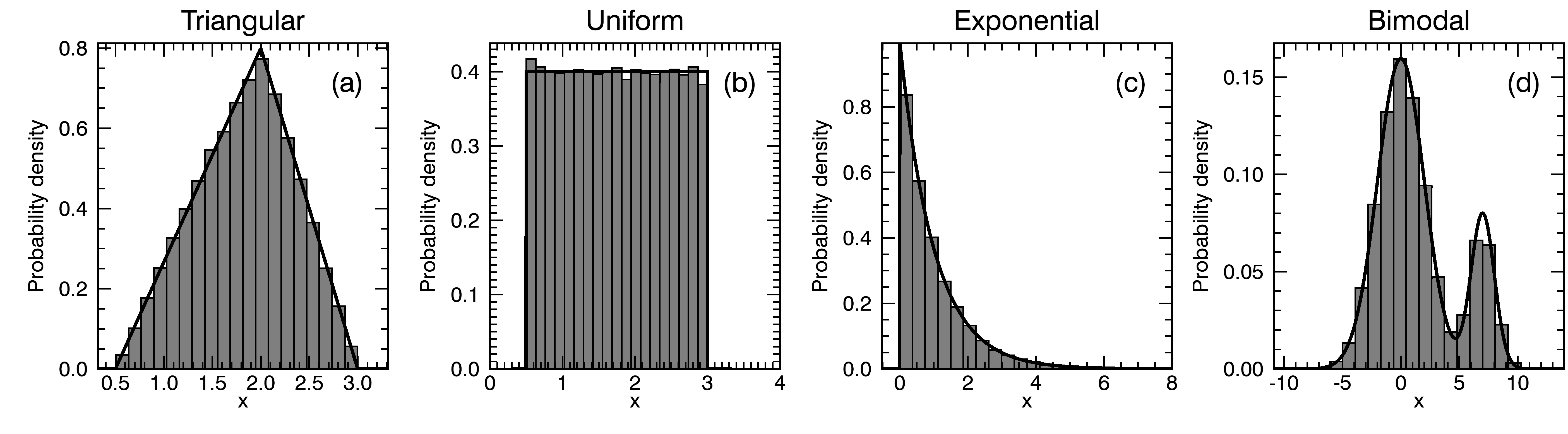
Figure 1: Normalised histograms of $10^{5}$ MCMC samples obtained from different univariate target distributions: asymmetric triangular (a), uniform (b), exponential (c), and mixture of two normal distributions (d). The target distributions are plotted over histograms with solid black lines.

4.2 2D target distributions

To demonstrate the correctness of the sampling procedure in multi parametric case, we present the testing results for a set of bivariate target probability densities. We selected 2D versions of the distributions used in 4.1: pyramid (Fig. 2a), 2D uniform distribution bounded by a square (Fig. 2a), 2D exponential distribution, and a mixture of 3 bivariate normal distributions with different expected values and covariance matrices. The 2D histograms (see Fig. 2) are perfectly coinciding with the target densities, shown in Fig. 2 by contours.

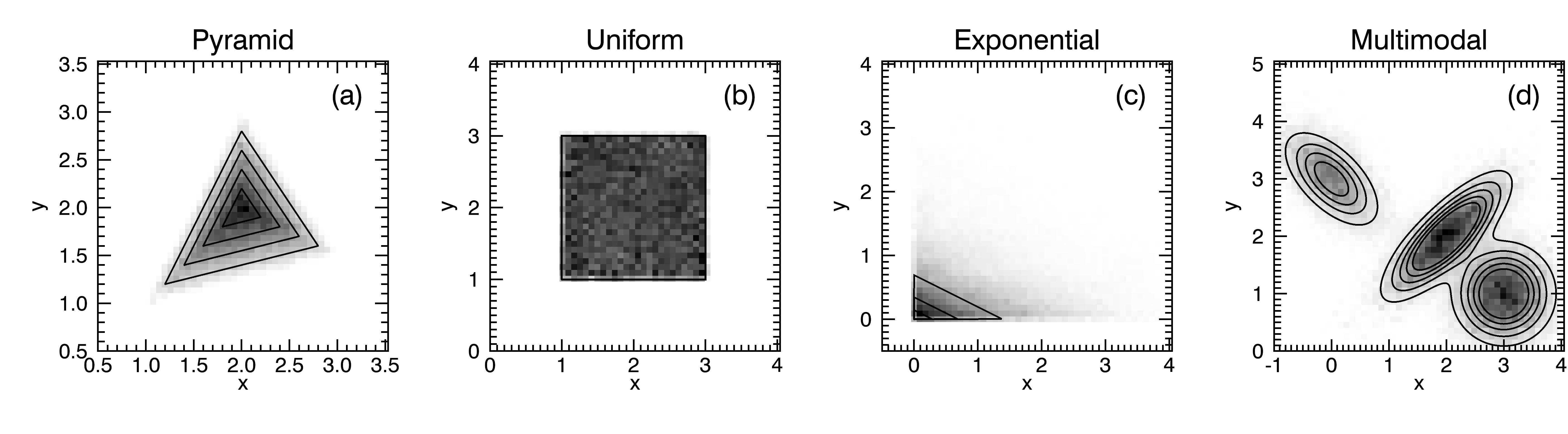
Figure 2: 2D histograms (background colour) of $10^{5}$ MCMC samples obtained from different bivariate target distributions: pyramid (a), uniform (b), exponential (c), and mixture of three normal distributions (d). The target distributions are shown by contours.

5 Examples of usage

In this section, we demonstrate examples of using SoBAT library to fit a simple linear dependence and consider an example of the Bayesian model comparison.

5.1 Fitting a linear dependence

Let us consider a simple example of fitting a set of synthetic data points ${X_{i},Y_{i}}$ by a linear function to illustrate the practical usage of SoBAT. The synthetic data points in our example are generated using the linear dependence with the present of the normally distributed noise

$$Y_{i}=kX_{i}+b+N(0,\sigma),$$

where $k=0.5$, $b=1$, and $\sigma=2$.

Firstly, we need to specify the model as a function describing the linear dependence of $y$ upon $x$. The model function for the linear dependence is given in Listing 1.

Listing 1: Model function for the linear dependence

⬇

1 function lin_model, x, params

2 k = params[0]

3 b = params[1]

4 return, k * x + b

5 end

Then, we define allowed limits as uniform priors and an initial guess for the model parameters $k$, $b$ (lines 2 – 6 in Listing 2). After the call of MCMC_FIT function (lines 12 – 14 in Listing 2), the variable fit will contain the best fitting values for $Y$. The fitted parameters values and corresponding uncertainties will be stored in the pars and credible_intervals variables. The MCMC samples will be returned in the samples keyword. The latter can be used to plot histograms approximating the marginalised posterior distributions. The histograms obtained for the slope ($k$), bias ($b$) and noise level ($\sigma$) are given in Figure 3 (b – d). Note, that the true parameter values (green vertical lines in Figure 3) do not coincide with global maximum of the histograms, but lie within the high probability area illustrated by histograms. Such a behaviour is expected because our inference (as any measurement) is uncertain. The uncertainty is described by the width of the histograms and can be quantified for an arbitrary level of significance by computing credible intervals as percentiles of the samples generated with the MCMC code.

Listing 2: Running MCMC fitting of the linear dependence for the data defined by Listing 1

⬇

1 ; define priors

2 priors = objarr(2)

3 priors[0] = prior_uniform(-5d, 5d)

4 priors[1] = prior_uniform(-5d, 5d)

5 ; define the initial guess

6 pars = [1d, 1d]

7 ; define the number of samples

8 n_samples = 100000

9 ; define the number of burn in samples

10 burn_in = 10000

11 ; run MCMC fitting

12 fit = mcmc_fit(x, y, pars, ”lin_model”, $

13 priors=priors, burn_in=burn_in, $

14 n_samples=n_samples, samples=samples, $

15 credible_intervals=credible_intervals)

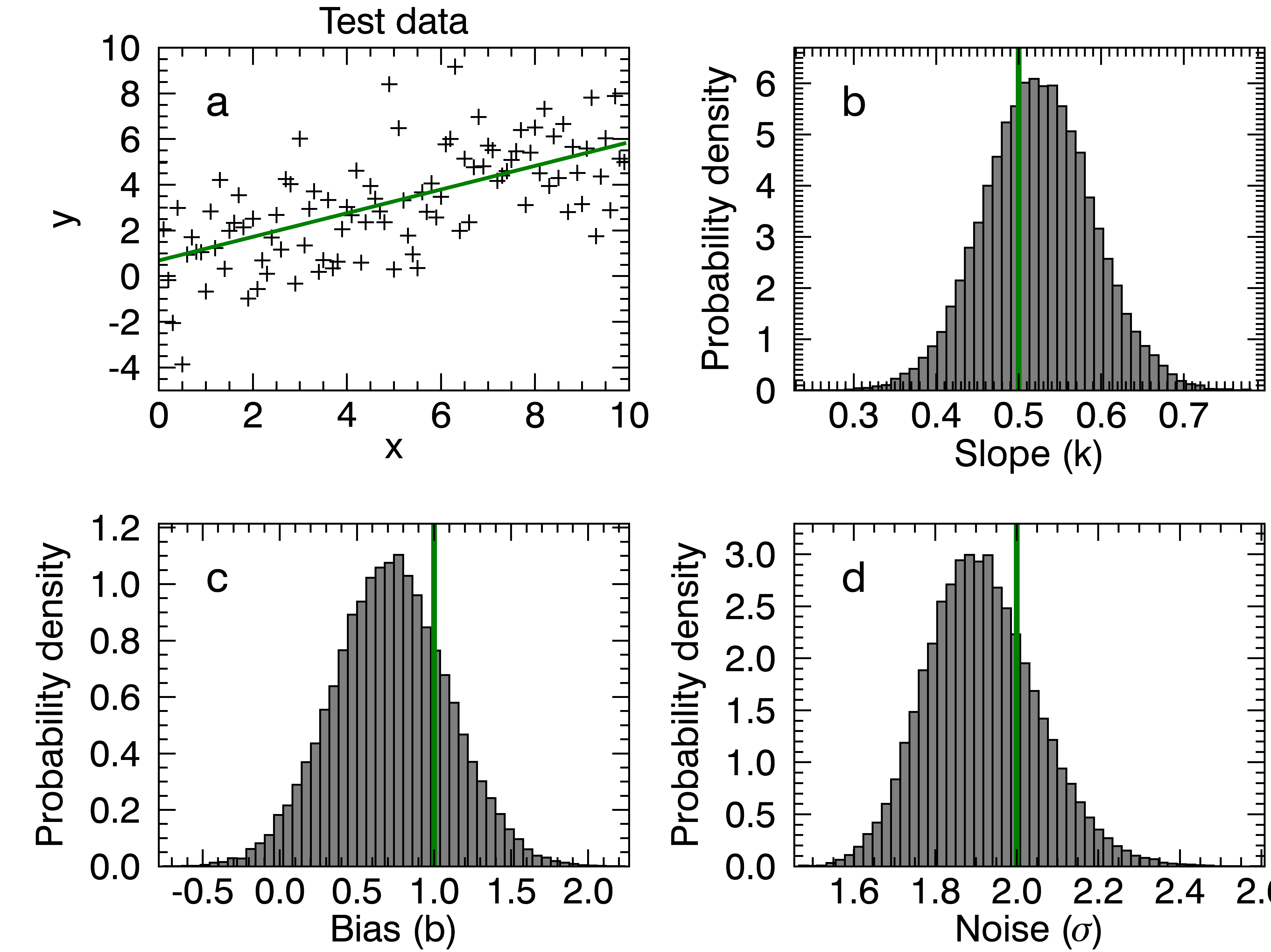
Figure 3: Panel a: linear dependence $y=kx+b$ (green line) fitted to the noisy synthetic data points (crosses) using the MCMC_FIT function. Panels b – d: normalised histograms approximating marginalised posterior distributions of the gradient $k$ (b), bias $b$ (c), and noise level $\sigma$ (d) obtained from $10^{5}$ MCMC samples. True values of the parameters used to generate synthetic data points are shown by vertical green lines on panels b–d.

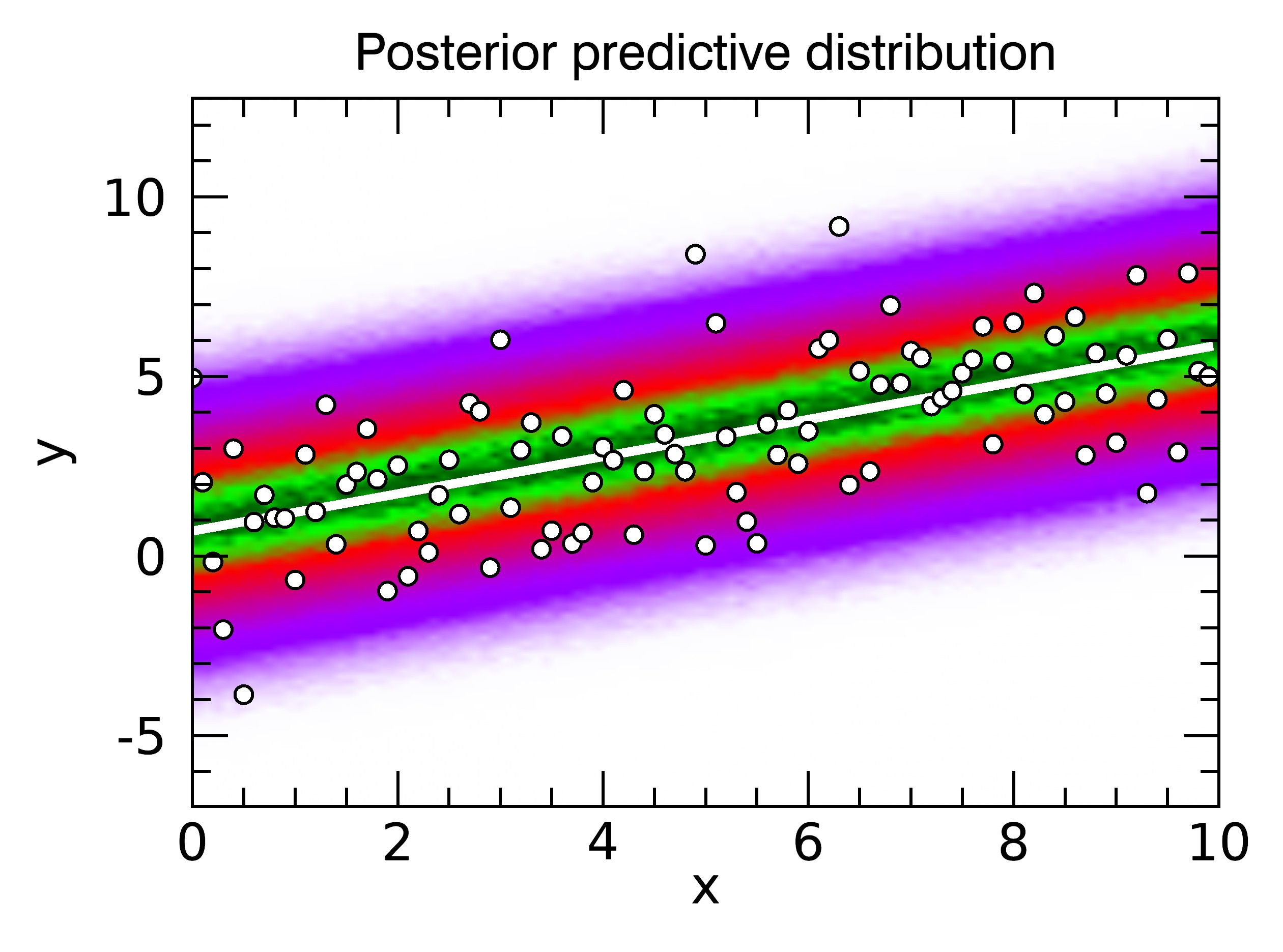
Figure 4: Posterior predictive probability distribution for a linear dependence fitted to the noisy synthetic data using the MCMC_FIT function. Data points are indicates by white circles while the white line shows the best fit.

5.2 Example of Bayesian model comparison

To illustrate quantitative comparison of different user-defined models, we use the same synthetic data set as in Sect. 5.1 with the linear dependence contaminated by white noise. Now we attempt to fit it with a second model with the quadratic dependence:

$$y=kx+b+cx^{2}+N(0,\sigma).$$ (11)

Listing 3 shows the IDL representation of this model.

Listing 3: Model function for the quadratic dependence

⬇

1 function quad_model, x, params

2 k = params[0]

3 b = params[1]

4 c = params[2]

5 return, k * x + b + c * x^2

6 end

The MCMC Bayesian inference is done for both models and then the models are compared by calculating the Bayes factor. Figures 5 and 6 show the MCMC inference results for the quadratic model given by Eq. (11). Though the best fits and posterior predictive distributions (see Figs 4 and 6) are very similar, the histograms of marginal posterior distributions are found to be significantly broader in comparison with the linear case. This demonstrates that the additional quadratic term does not improve the fit. The $\chi^{2}$ and reduced $\chi^{2}$ metrics are almost the same for both models (see Table 1) and do not show any significant advantage of one model against the other.

SoBAT includes the MCMC_EVIDENCE function which allows us to calculate Bayesian evidences and hence the Bayes factor for comparing the models as described in Listing 4, where samples_l and samples_q are the MCMC samples simulated using the linear and quadratic models, respectively. The computed Bayes factor ($28.8$) indicates strong evidence in the favour of the linear model. This result is expected since we generated the synthetic data using the linear dependence with the background normally distributed noise.

Listing 4: Calculating the Bayes factor

⬇

1 e_l = mcmc_fit_evidence(samples_l,$

2 x, y, priors, ’lin_model’)

3 e_q= mcmc_fit_evidence(samples_q,$

4 x, y, priors, ’quad_model’)

5 Bayes_factor = e_l/e_q

Table 1: Quantitative comparison of the linear and quadratic models

Model	Chi-squared	Reduced chi-squared	Evidence	Bayes factor
$M_{1}$: Linear	346.8	3.539	$4.7\times 10^{-94}$	$28.8$
$M_{2}$: Quadratic	346.2	3.569	$1.6\times 10^{-95}$	$-28.8$

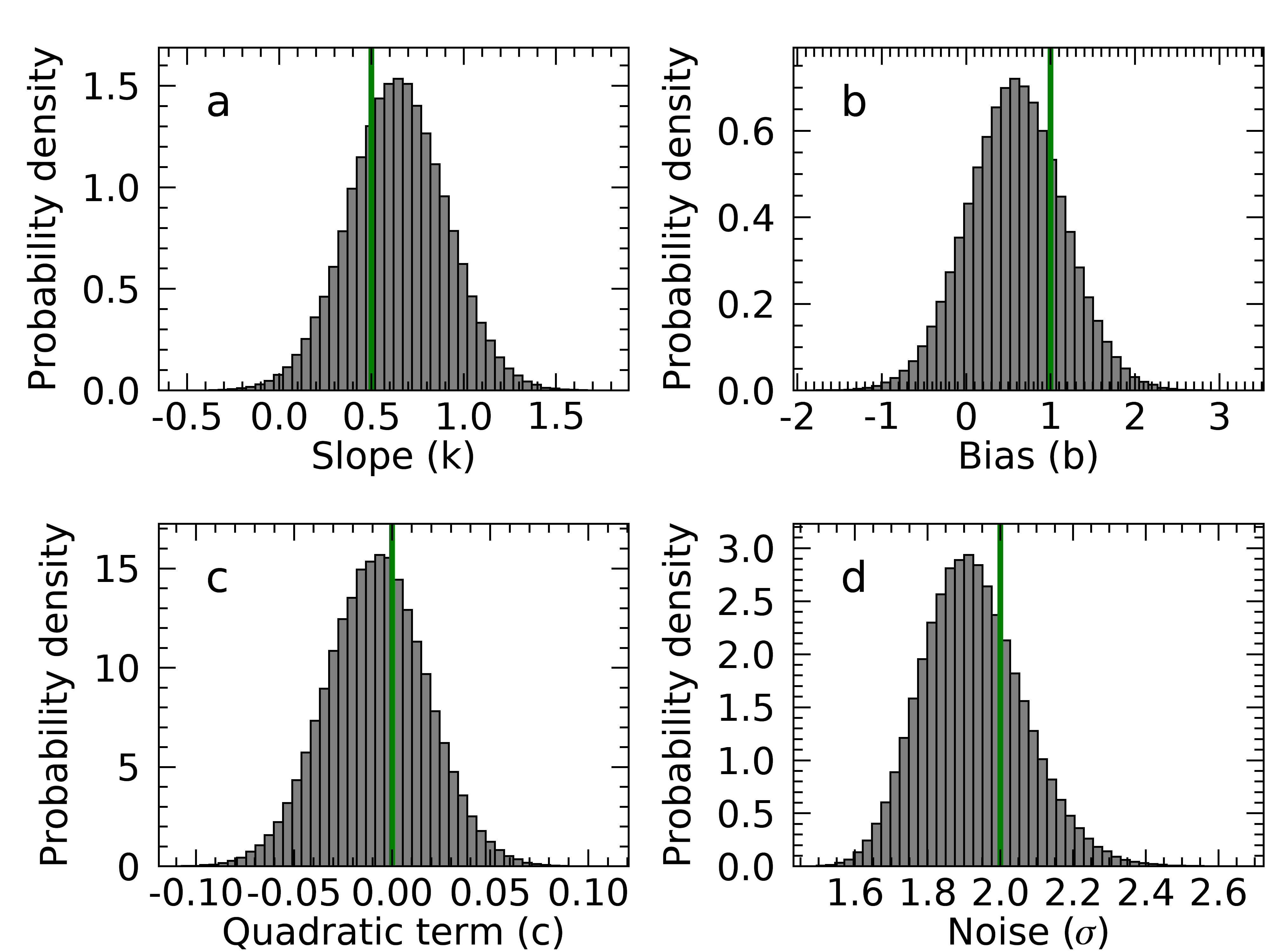
Figure 5: Panel a: Normalised histograms approximating marginalised posterior distributions of the slope $k$ (a), bias $b$ (b), quadratic term $c$ (c) and noise level $\sigma$ (d) obtained from $10^{5}$ MCMC samples using the quadratic model $y=kx+b+cx^{2}$. True values of the parameters used to generate synthetic data points are shown by vertical green lines.

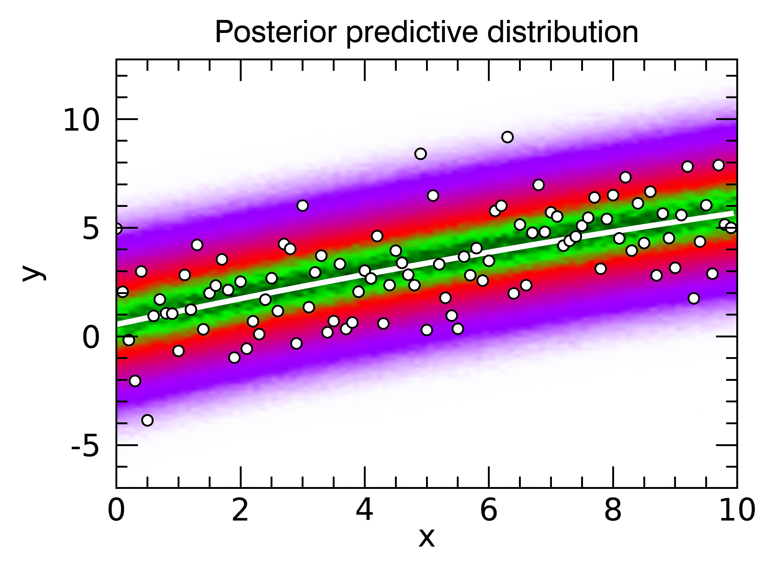
Figure 6: Posterior predictive probability distribution for a quadratic dependence fitted to the noisy synthetic data using the MCMC_FIT function. Data points are indicates by white circles while the white line shows the best fit.

6 Application to realistic problems

In this section we illustrate the application of SoBAT to problems in solar physics.

6.1 Coronal loop seismology using damped kink oscillations

Coronal loops are frequently observed to perform large amplitude, rapidly-damped, transverse oscillations when perturbed by events such as flares and coronal mass ejections. Their rapid damping is explained by resonant absorption which causes a transfer of energy from the kink mode to the torsional Alfvén mode (e.g. see the recent review by De Moortel et al., 2016). Pascoe et al. (2013) proposed a method to infer the transverse density profile in the oscillating coronal loop using the shape of the damping profile of the kink oscillation (Hood et al., 2013; Pascoe et al., 2012, 2015, 2016a, 2019). The method was first applied in Pascoe et al. (2016b) using a Levenberg-Marquardt least-squares fit to the data using the IDL code MPFIT (Markwardt, 2009). It was extended in Pascoe et al. (2017a) to include additional physical effects and also use Bayesian inference. Pascoe et al. (2017c) also included the presence of a large initial displacement of the loop equilibrium position. A benefit of the MCMC approach is that we can readily extend our models in this way, allowing us to investigate further details in the data.

We note that in previous applications of our MCMC code to coronal seismology (Pascoe et al., 2017a, b, c; Goddard et al., 2017), posterior summaries were given using the median value (and uncertainties by the 95% credible interval). Here, as well as in Pascoe et al. (2018), the maximum a posteriori probability (MAP) estimate is used rather than the median.

In this paper, we use the simplified version of the oscillation profile model published in Pascoe et al. (2017a):

$$y(t)=y_{\rm tr}(t)+\left\{\begin{matrix}A_{0}e^{-\left(\frac{\tilde{t}}{\tau}\right)^{n}}\sin\left(\frac{2\pi\tilde{t}}{P}+\phi_{0}\right),&\tilde{t}\geq 0\\ x_{0},&\tilde{t}<0\end{matrix}\right.,$$ (12)

where $\phi_{0}=\arcsin(\frac{x_{0}}{A_{0}})$ is the initial phase, $A_{0}$ is the initial amplitude, $t_{0}$ is the start time of the oscillation, $\tilde{t}=t-t_{0}$, $P$ is the oscillation period, and $x_{0}$ is the initial displacement which prescribes the oscillation phase. The parameter $n$ prescribes the damping profile. The background trend ($y_{\rm tr}$) prescribes the equilibrium position and is calculated using spline interpolation from the reference points located at the time instances when the loop comes through the equilibrium (blue diamonds in Figure 7). The positions of the reference points are free parameters of the model and are identified during the Bayesian inference. [give listings in appendix]

As an example, we consider the time series of the loop position taken for Event 43 Loop 3 from the catalogue of oscillations by Goddard et al. (2016). This loop is also referred to as Loop #1 in the seismological analysis by Pascoe et al. (2016b, 2017a). The observational data points and the best fit obtained using the MCMC_FIT function are shown in Figure 7. The histograms approximating marginal posterior distributions of oscillation period, amplitude, decay time, initial displacement, start time, and the position of a trend reference point are given in Figure 8.

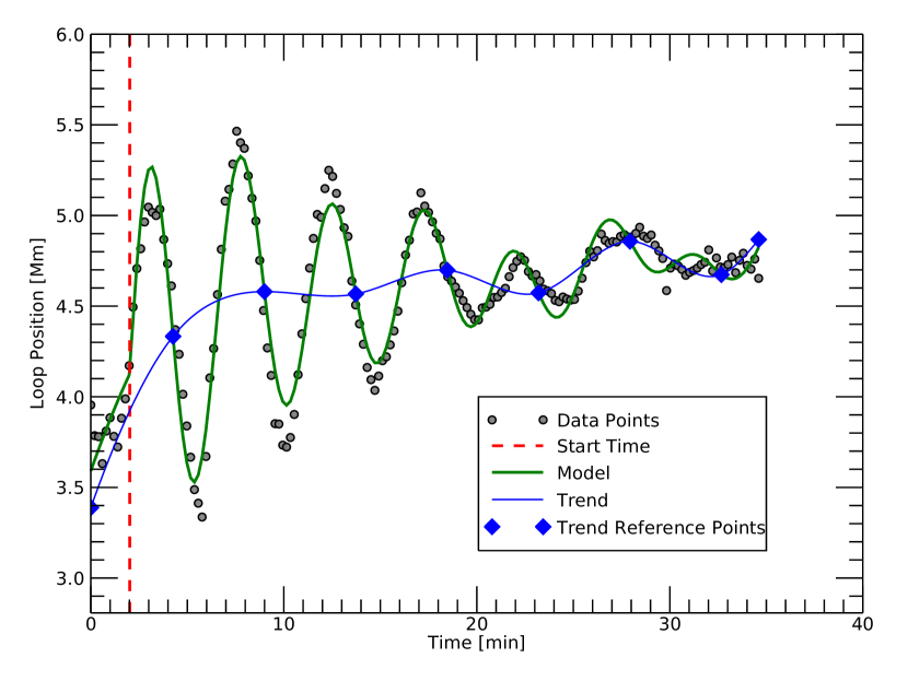
Figure 7: Best fit (green line) computed for the simplified model of decaying kink oscillations. Observational data points are shown by grey circles. The inferred background trend computed by spline interpolation from the reference points (blue diamonds) is shown by a blue line. The vertical red dashed line denotes the oscillation start time.

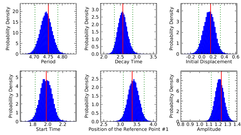
Figure 8: Histograms approximating marginalised posterior PDF obtained using the MCMC_FIT routine for the simplified model of exponentially decaying kink oscillations. The MAP estimates are indicated with the vertical red lines, while the dotted lines show 95% credible intervals.

The Posterior Predictive distribution inferred using our MCMC code is given in Figure 9. The shaded area demonstrates the region on the plot where the data points are predicted to be observed. For a data consistent inversion, the measured data points should be located inside the shaded region and the shaded area itself should not broaden far away from the data points. That means that a model should predict the observed data points, but it should not predict observations being far away from the actually observed data.

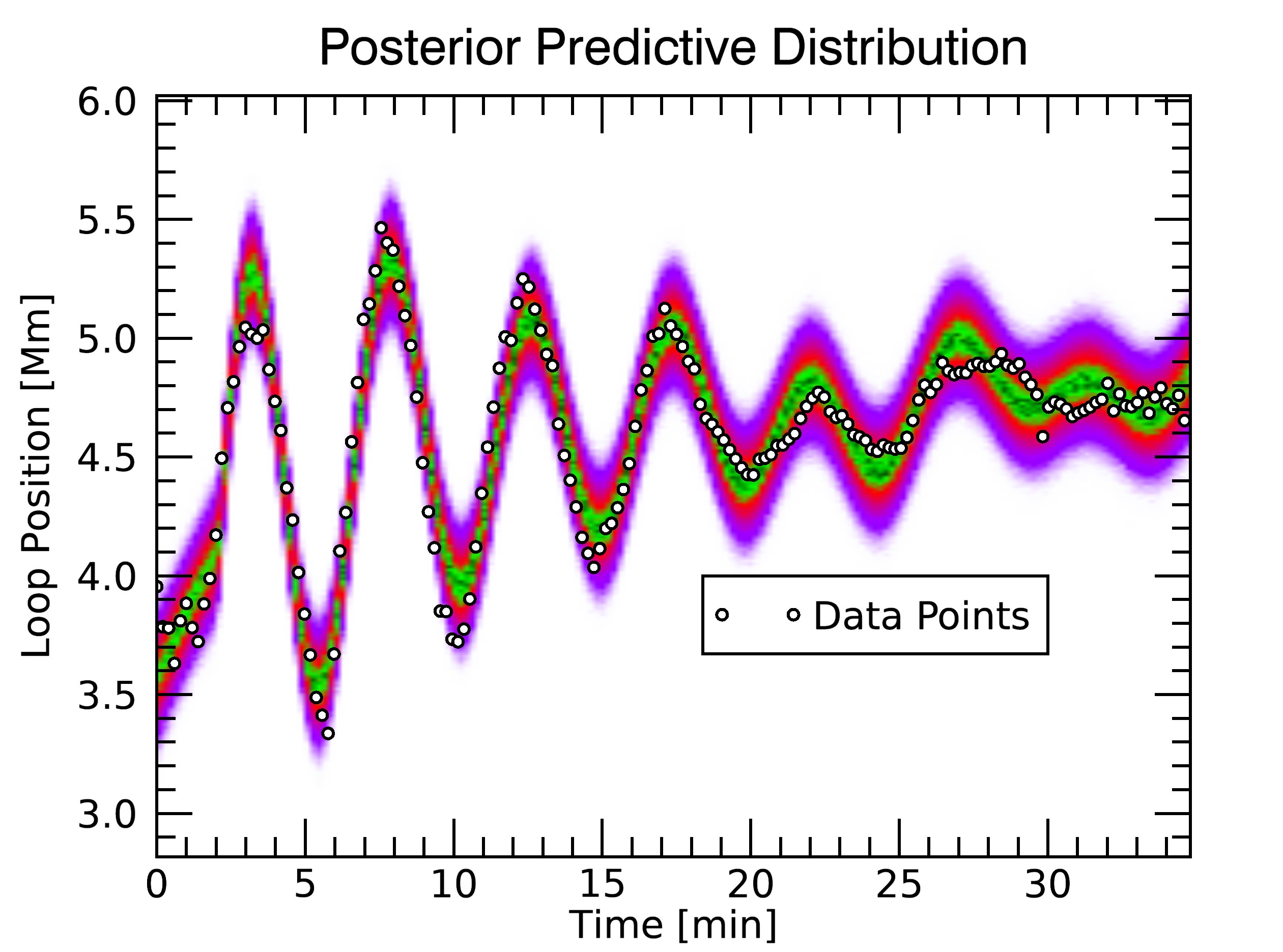
Figure 9: Posterior predictive distribution PDF (background colour) over-plotted with the observed data points (circles).

7 Conclusions

In this paper, we have described a new code written in IDL to perform MCMC sampling and Bayesian inference for the purpose of testing data against one or more models. This method and code is applicable to a wide range of problems. It requires that the user supplies a function which returns the predicted values of the data using model parameters, and the prior ranges for these parameters. These priors may either be prescribed limits for the parameter, or else reasonable estimates for the data being considered.

Since the method is based on forward modelling of the data and efficient sampling of the parameter space it is able to describe model parameters which have arbitrary posterior probability distributions. This allows reliable estimations of the values and uncertainties of model parameters. Furthermore, it allows the method to accommodate both well-posed and ill-posed problems. This is convenient for attempts to reliably extract the maximum information from the available data. For example, the seismological method of determining the density profile of coronal loops using damped kink oscillations uses the shape of the damping profile to make the problem well-posed. In the case of the data not supporting a reliable determination of the shape, the problem reverts to being ill-posed and the MCMC sampling recovers an inverse relationship between the density contrast and inhomogeneous layer width (see Pascoe et al., 2018, for further discussion).

Our code has also been used to estimate the density profile of a coronal loop (Pascoe et al., 2017b, 2018; Goddard et al., 2017) using a simple procedure for forward modelling the extreme ultraviolet (EUV) emission based on the isothermal approximation (e.g. Aschwanden et al., 2007), and recently applied to the problem of analysing quasi-periodic pulsations in solar and stellar flares (Broomhall et al., 2019).

The Bayesian evidence may be used to compare two or more competing models for the same data. In comparison to other tests such as the (reduced) chi-squared, its robustness is increased by considering all prior and posterior information rather than simply the goodness of the model best fits.

The code is available at GitHub page https://github.com/Sergey-Anfinogentov/SoBAT. According to our knowledge it is the only avialable MCMC code written in IDL which is ready to use out of the box. Example of the code usage in appendix and also available at GitHub.

Appendix A Listing of kink oscillation parameter inference

Listing 5: Running MCMC fitting of Decaying sinusoid into the observed displacements of the oscillating coronal loop

⬇

1 pro kink_example_data, x, y

2 ;observational data points

3 x = [0.00,0.20,0.40,0.60,0.80,0.99,1.19,1.39,1.59,1.79,1.99,2.19,$

4 2.39,2.59,2.78,2.98,3.18,3.38,3.58,3.78,3.98,4.18,4.38,4.57,$

5 4.77,4.97,5.17,5.37,5.57,5.77,5.97,6.16,6.36,6.56,6.76,6.96,$

6 7.16,7.36,7.56,7.76,7.95,8.15,8.35,8.55,8.75,8.95,9.15,9.35,$

7 9.55,9.74,9.94,10.14,10.34,10.54,10.74,10.94,11.14,11.34,11.53,$

8 11.73,11.93,12.13,12.33,12.53,12.73,12.93,13.13,13.32,13.52,$

9 13.72,13.92,14.12,14.32,14.52,14.72,14.92,15.11,15.31,15.51,$

10 15.71,15.91,16.11,16.31,16.51,16.70,16.90,17.10,17.30,17.50,$

11 17.70,17.90,18.10,18.30,18.49,18.69,18.89,19.09,19.29,19.49,$

12 19.69,19.89,20.09,20.28,20.48,20.68,20.88,21.08,21.28,21.48,$

13 21.68,21.88,22.07,22.27,22.47,22.67,22.87,23.07,23.27,23.47,$

14 23.67,23.86,24.06,24.26,24.46,24.66,24.86,25.06,25.26,25.45,$

15 25.65,25.85,26.05,26.25,26.45,26.65,26.85,27.05,27.24,27.44,$

16 27.64,27.84,28.04,28.24,28.44,28.64,28.84,29.03,29.23,29.43,$

17 29.63,29.83,30.03,30.23,30.43,30.63,30.82,31.02,31.22,31.42,$

18 31.62,31.82,32.02,32.22,32.42,32.61,32.81,33.01,33.21,33.41,$

19 33.61,33.81,34.01,34.21,34.40,34.60]

20 y = [3.95,3.79,3.78,3.63,3.81,3.88,3.78,3.72,3.88,3.99,4.17,4.49,$

21 4.71,4.82,4.96,5.05,5.02,5.00,5.03,4.87,4.73,4.61,4.37,4.23,$

22 4.01,3.84,3.67,3.49,3.41,3.34,3.67,4.10,4.27,4.56,4.81,5.08,$

23 5.14,5.28,5.46,5.40,5.37,5.22,5.10,4.97,4.75,4.48,4.27,4.12,$

24 3.85,3.85,3.73,3.72,3.78,3.90,4.12,4.35,4.54,4.71,4.87,5.01,$

25 4.99,5.15,5.25,5.22,5.12,5.03,4.93,4.88,4.64,4.51,4.40,4.29,$

26 4.16,4.09,4.04,4.11,4.20,4.22,4.29,4.36,4.47,4.63,4.78,4.86,$

27 5.01,5.02,5.13,5.05,5.02,4.97,4.90,4.87,4.72,4.66,4.64,4.61,$

28 4.57,4.53,4.49,4.46,4.43,4.42,4.49,4.50,4.51,4.55,4.55,4.57,$

29 4.60,4.66,4.71,4.75,4.77,4.75,4.69,4.67,4.67,4.64,4.59,4.58,$

30 4.57,4.53,4.52,4.55,4.54,4.53,4.54,4.58,4.65,4.74,4.80,4.77,$

31 4.81,4.90,4.86,4.85,4.86,4.85,4.88,4.89,4.88,4.88,4.90,4.94,$

32 4.89,4.87,4.89,4.84,4.80,4.76,4.59,4.71,4.73,4.72,4.70,4.67,$

33 4.69,4.70,4.71,4.73,4.74,4.81,4.69,4.77,4.72,4.71,4.73,4.77,$

34 4.68,4.75,4.79,4.72,4.70,4.76,4.65]

35 end

36

37 ; model function accepts keyword parameter N_TREND

38 ; that will be passed to it

39 function model_exp_decay, x, a, n_trend=n_trend

40 tstart = a[0] ; oscillation start time

41 period = a[1] ; oscillation period

42 q_factor = a[2] ; oscillation decay_time

43 amp = a[3] ; initial amplitude

44 displ = a[4]

45 ref_y = a[5:5+n_trend-1] ; trend reference points

46 ref_x = linspace(x[0],x[-1],n_trend)

47 tau = q_factor*period ; decay time

48 tosc = x-tstart

49 omega = 2.d*!dpi/period

50 phi = asin((displ)) ; initial phase

51 ; decaying profile

52 damp = amp * exp(-(tosc/tau)^1) * (x ge tstart)

53 oscillation = damp * sin(omega*(tosc>0d) + phi)

54 trend = spline(ref_x, ref_y, x)

55 return, trend + oscillation

56 end

57

58 pro example_kink

59 kink_example_data, x, y

60 plot, x, y, /psym

61 ; use 5 reference points for the trend

62 n_trend = 5

63 ; initial values

64 pars = [1d, 2d, 2d, 1d, 0d, 5d, 5d, 5d, 5d, 5d]

65 priors = [$

66 prior_uniform(0d, 5d), $ ; start time

67 prior_uniform(1d, 10d), $ ; period

68 prior_uniform(1d, 10d), $ ; q factor

69 prior_uniform(0d, 10d), $ ; amplitude

70 prior_uniform(-1d, 1d), $ ; initial displacement

71 ; trend reference points

72 replicate(prior_uniform(min(y), max(y)), n_trend) $

73 ]

74 model = ’model_exp_decay’

75 ; sample posterior distribution using the MCMC

76 y_fit = mcmc_fit(x, y, pars, model, n_samples = 100000l, priors=priors, $

77 burn_in=50000l, samples=samples, n_trend=n_trend)

78 end

References

- Arregui (2018) Arregui, I. 2018, Advances in Space Research, 61, 655, doi: 10.1016/j.asr.2017.09.031
- Aschwanden et al. (2007) Aschwanden, M. J., Nightingale, R. W., & Boerner, P. 2007, ApJ, 656, 577, doi: 10.1086/510232
- Broomhall et al. (2010) Broomhall, A.-M., Chaplin, W. J., Elsworth, Y., Appourchaux, T., & New, R. 2010, MNRAS, 406, 767, doi: 10.1111/j.1365-2966.2010.16743.x
- Broomhall et al. (2019) Broomhall, A.-M., Davenport, J. R. A., Hayes, L. A., et al. 2019, The Astrophysical Journal Supplement Series, 244, 44, doi: 10.3847/1538-4365/ab40b3
- De Moortel et al. (2016) De Moortel, I., Pascoe, D. J., Wright, A. N., & Hood, A. W. 2016, Plasma Physics and Controlled Fusion, 58, 014001
- Goddard et al. (2016) Goddard, C. R., Nisticò, G., Nakariakov, V. M., & Zimovets, I. V. 2016, A&A, 585, A137, doi: 10.1051/0004-6361/201527341
- Goddard et al. (2017) Goddard, C. R., Pascoe, D. J., Anfinogentov, S., & Nakariakov, V. M. 2017, A&A, 605, A65, doi: 10.1051/0004-6361/201731023
- Hastings (1970) Hastings, W. K. 1970, Biometrika, 57, 97, doi: 10.1093/biomet/57.1.97
- Hood et al. (2013) Hood, A. W., Ruderman, M., Pascoe, D. J., et al. 2013, A&A, 551, A39, doi: 10.1051/0004-6361/201220617
- Howe et al. (2015) Howe, R., Davies, G. R., Chaplin, W. J., Elsworth, Y. P., & Hale, S. J. 2015, MNRAS, 454, 4120, doi: 10.1093/mnras/stv2210
- Jeffreys (1961) Jeffreys, H. 1961, Theory of Probability, 3rd edn. (Oxford). /bib/jeffreys/Jeffreys1961/%5BJeffreys_H.%5D_Theory_of_probability%28BookZZ.org%29.djvu,/bib/jeffreys/Jeffreys1961/%5BHarold_Jeffreys%5D_Theory_of_probability%2C_3rd_Editi%28BookZZ.org%29.pdf
- Kass & Raftery (1995) Kass, R. E., & Raftery, A. E. 1995, Journal of the American Statistical Association, 90, 773, doi: 10.1080/01621459.1995.10476572
- Markwardt (2009) Markwardt, C. B. 2009, in Astronomical Society of the Pacific Conference Series, Vol. 411, Astronomical Data Analysis Software and Systems XVIII, ed. D. A. Bohlender, D. Durand, & P. Dowler, 251
- Pascoe et al. (2017a) Pascoe, D. J., Anfinogentov, S., Nisticò, G., Goddard, C. R., & Nakariakov, V. M. 2017a, A&A, 600, A78, doi: 10.1051/0004-6361/201629702
- Pascoe et al. (2018) Pascoe, D. J., Anfinogentov, S. A., Goddard, C. R., & Nakariakov, V. M. 2018, ApJ, 860, 31, doi: 10.3847/1538-4357/aac2bc
- Pascoe et al. (2017b) Pascoe, D. J., Goddard, C. R., Anfinogentov, S., & Nakariakov, V. M. 2017b, A&A, 600, L7, doi: 10.1051/0004-6361/201730458
- Pascoe et al. (2016a) Pascoe, D. J., Goddard, C. R., Nisticò, G., Anfinogentov, S., & Nakariakov, V. M. 2016a, A&A, 585, L6, doi: 10.1051/0004-6361/201527835
- Pascoe et al. (2016b) —. 2016b, A&A, 589, A136, doi: 10.1051/0004-6361/201628255
- Pascoe et al. (2012) Pascoe, D. J., Hood, A. W., de Moortel, I., & Wright, A. N. 2012, A&A, 539, A37, doi: 10.1051/0004-6361/201117979
- Pascoe et al. (2013) Pascoe, D. J., Hood, A. W., De Moortel, I., & Wright, A. N. 2013, A&A, 551, A40, doi: 10.1051/0004-6361/201220620
- Pascoe et al. (2019) Pascoe, D. J., Hood, A. W., & Van Doorsselaere, T. 2019, Frontiers in Astronomy and Space Sciences, 6, 22, doi: 10.3389/fspas.2019.00022
- Pascoe et al. (2017c) Pascoe, D. J., Russell, A. J. B., Anfinogentov, S. A., et al. 2017c, A&A, 607, A8, doi: 10.1051/0004-6361/201730915
- Pascoe et al. (2015) Pascoe, D. J., Wright, A. N., De Moortel, I., & Hood, A. W. 2015, A&A, 578, A99, doi: 10.1051/0004-6361/201321328
- Sharma (2017) Sharma, S. 2017, ARA&A, 55, 213, doi: 10.1146/annurev-astro-082214-122339