Observation of multiple sausage oscillations in cool postflare loop

Abstract

Using simultaneous high spatial (1.3 arc sec) and temporal (5 and 10 s) resolution H-alpha observations from the 15 cm Solar Tower Telescope at ARIES, we study the oscillations in the relative intensity to explore the possibility of sausage oscillations in the chromospheric cool postflare loop. We use standard wavelet tool, and find the oscillation period of $\approx$ 587 s near the loop apex, and $\approx$ 349 s near the footpoint. We suggest that the oscillations represent the fundamental and the first harmonics of fast sausage waves in the cool postflare loop. Based on the period ratio $P_{1}/P_{2}\sim$ 1.68, we estimate the density scale height in the loop as $\sim$ 17 Mm. This value is much higher than the equilibrium scale height corresponding to H-alpha temperature, which probably indicates that the cool postflare loop is not in hydrostatic equilibrium. Seismologically estimated Alfvén speed outside the loop is $\sim$ 300-330 km/s. The observation of multiple oscillations may play a crucial role in understanding the dynamics of lower solar atmosphere, complementing such oscillations already reported in the upper solar atmosphere (e.g., hot flaring loops).

1 Introduction

The coupling of complex magnetic field and plasma generates variety of magnetohydrodynamic (MHD) waves and oscillations in various solar structures. These MHD waves and oscillations are one of the important candidates for coronal heating and solar wind acceleration. The idea of exploiting observed oscillations as a diagnostic tool for determining the physical conditions of the coronal plasma was first suggested by Roberts et al. (1984). Until recently, the application of this idea has been marked by the lack of high-quality observations of coronal oscillations. However, this situation has changed dramatically, especially due to space-based observations by the Solar and Heliospheric Observatory (SOHO), the Transition Region and Coronal Explorer (TRACE), and most recently with the high resolution spectra from the Hinode spacecraft. The fast kink wave is most frequently observed mode as it can be directly detected by periodic spatial displacement of coronal loop axis (Nakariakov et al. 1999; Aschwanden et al. 1999; Wang & Solanki 2004). Using temporal series image data from CDS/SOHO, recently O’Shea et al. (2007) have found the first evidence of fast-kink standing oscillations in the cool transition region loops as well. On the other hand, the fast MHD sausage wave causes the variation of pressure and magnetic field in a coronal loop and therefore can be observed as intensity oscillations or periodic modulation of coronal radio emission (Nakariakov et al. 2003). Recently, Srivastava et al. (2008) have reported the signature of the leakage of chromospheric magnetoacoustic oscillations into the corona near the south pole. These observations provide a basis for the estimation of coronal plasma properties (Nakariakov & Ofman 2001).

Recently, Verwichte et al. (2004) have detected interesting phenomenon of simultaneous existence of fundamental and first harmonics of fast kink oscillations (see also De Moortel & Brady 2007; Van Doorsselaere et al. 2007). However, the ratio between the periods of fundamental and first harmonics $P_{1}/P_{2}$ was significantly shifted from 2, which later was explained as a result of longitudinal density stratification in the loop (Andries et al. 2005; McEwan et al. 2006). The rate of the shift allows to estimate the density scale height in coronal loops, which can be few times larger compared to its hydrostatic value (Aschwanden et al. 2000).

In this paper, we report the first evidence of fundamental and first harmonics of fast sausage oscillations in cool postflare loop. We use high spatial (1.3 arc sec) and temporal (5 and 10 s) resolution H-alpha observations from the 15 cm Solar Tower Telescope at ARIES, Nainital, India, to study the oscillations in the relative intensity. Using the standard wavelet tool, we find multiple oscillation periods at different parts of the loop, which are interpreted as the fundamental and first harmonics of fast sausage mode. In section 2, we describe the observations and data reduction. We describe the wavelet analysis in section 3. In section 4, we present our theoretical model and its link to coronal seismology. We present results and discussion in the last section.

2 Observations and data reduction

The observations of post flare loops have been carried out with 15 cm, f/15 Coudé Solar Tower Telescope at ARIES, Nainital, India, equipped with Bernhard Hale H-alpha filter ($\lambda$ = 6563 Å  and P.B. 0.5/0.7 Å ), and PXL Photometric CCD camera. The filter is a birefringent Lyot type filter, tunable $\pm$ 1 Å from central wavelength (6563 Å ) with the step of 0.1 Å . During our observations, we set it at central wavelength 6563 Å with passband 0.5 Å . The Image size has been enlarged by a factor of two using a Barlow lens. The 512 $\times$ 512 pixels, 12-bit frame transfer CCD camera has a square pixel of 15 $\mu$m² corresponding to a 0.65 arc sec pixel size. The spatial resolution of our observations is 1.30 arc sec. The read out noise for the system is 31 e^- with a gain of 44.1 e^-/ADU. Dark current of the camera is 56 e${}^{-}s^{-1}$. The dark current is integrated over the 512 x 512 pixels. The camera controller of the system has a variable read-out rate from 0.5 to 2 MHz.The variable read out rate of our CCD provides us the facility of fast imaging of the flares at different rates. In these observations, we have used a constant read out rate of 2 MHz. The The CCD chip (EEV 37) is cooled up to -25^o C using liquid cooling system.

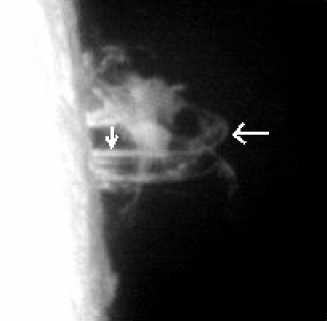
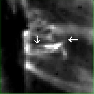
Figure 1: The H-alpha post flare loops as observed by 15 cm Solar Tower Telescope at ARIES, Nainital, India. The FOV is 200 pixel $\times$ 200 pixel (or 130 arc sec $\times$ 130 arc sec) (left panel).The aligned SOHO/EIT Fe IX/X 171 Å image of the same loop system is presented in right panel.

We analyze the postflare loop system between 01:00:52 U.T. and 01:58:28 UT on May 2, 2001, at a cadence of 5 s and 10 s with an exposure time of 30 ms. The post flare loop system was associated with M1.8 class limb flare which occured in NOAA active region AR 9433 (N15, W88). Since, the temporal evolution/changes were very fast during the onset of post flare loop system, we took fast sequence of images with 5 s cadence. As time progresses in the gradual/decay phase, the temporal changes become slow compared to initial phase of post flare loop system. So, we took the sequence of images with 10 s cadence. Hence, there are two cadences, initially 5 s and later on 10 s. We have started our fast imaging with 5 s cadence on 00:52:11 UT. In the beginning of our observations, the flare was in decay phase and was enveloped by complex post flare loop system. Hence, we were unable to select the distinct loop initially. The post flare loop system became more relaxed and distinctly visible around 01:00:52 UT, then we have selected images of a clearly visible loop for our study after 01:00:52 UT. In our analysis, first 92 frames were with 5 s cadence, while rest of the frames were with 10 s cadence. The total number of the frames used in this study is 390. We find that the post flare loop system shows the similar structure/evolution in SOHO/EIT (171 Å , 195 Å , 284 Å , 304 Å ) and H-alpha observations.The post flare loop system which was visible at higher temperature (6.0$\times$10⁴ K–3.0$\times$10⁶ K) with EIT, has also seen in H-alpha at the lower temperature ($\approx$ 10⁴ K) after its cooling. In Fig 1 (top panel), the image of the post flare loop system in high resolution H-alpha has been shown, while the same loop system observed with SOHO/EIT Fe IX/X 171 Å has been shown in the bottom panel.Both images show the clear shape of the dynamic post flare loop that we have selected. The loop top and foot point of this prominent loop marked by arrows in these two images. Since the spatial resolution of our H-alpha observations is high in comparison to the SOHO/EIT, hence we can not see the features in EIT as sharp as in H-alpha image.

We have estimated the length of the selected loop in H-alpha and SOHO/EIT Fe IX/X 171 Å images. We find the lengths $\sim$ 97 Mm and $\sim$ 100 Mm in the H-alpha and EUV images respectively. The estimated loop lengths at two wavelengths are almost equal which clearly shows the presence of the same loop at different temperatures. The lower atmosphere may not necessarily be an optically thin atmosphere, and many bright structures cross to each other in the field of view. However, the chromospheric post flare loop system is very complex and dynamic in itself, instead of simpler and static. The features are temporally changing very fast in the observations. So, we carefully selected the image frames of the clearly visible loop in order to study the oscillations. The sky condition was very good during the observations. Several dark and flat field images have also been taken to calibrate the H-alpha images. Using IRAF and SSWIDL softwares, the image processing has been performed. The details of the instrument can be obtained from Ali et al. (2007) and Joshi et al. (2003).

3 Wavelet Analysis

We use the Morlet wavelet tool to produce the power spectrum of oscillations in H-alpha. The Morlet wavelet suffers from the edge effect of time series data. This effect is significant in regions defined as cone of influence (COI). The details of wavelet procedure, its noise filtering, COI effects etc. are given in Torrence & Compo (1998). Randomisation technique evaluates the peak power in the global wavelet spectrum, which is just the average peak power over time and similar to a smoothed Fourier power spectrum. This technique compares it to the peak powers evaluated from the $n!$ equally likely permutations of the time series data, assuming that n values of measured intensities are independent of n measured times if there is no periodic signal. The proportion of permutations which gives the value greater or equal to the original peak power of the time series, will provide the probability of no periodic component (p). The percentage probability

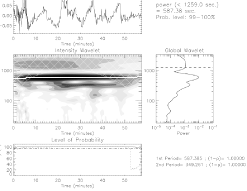
Figure 2: The wavelet result for H-alpha 6563 Å line near the loop apex. The top panel shows the variation of intensity, the wavelet power spectrum is given in the middle panel, and the probability in the bottom panel. The light curve is from the loop apex (X,Y) = (133th pixel, 117th pixel), and smoothed by window width 60.

of periodic components presented in the data will be $(1-p)\times 100$, and 95 % is the lowest acceptable probability for real oscillations. We set 200 permutations for the reliable estimation of p, and hence the probability of real oscillations. The details of randomisation technique to obtain the statistically significant real oscillation periods are given by Nemec & Nemec (1985) and O’Shea et al. (2001). We do not remove any upper/longer period intervals and associated powers of our time series data during wavelet analysis. We choose the ’running average’ option of O’Shea’s wavelet tool, and smooth the original signal by window width 60. Average smoothing process is used to reduce the noise in the original signal in order to get a real periodicity, and it is based on the low pass filtering methods. The ’Running Average’ process smooth the original signal by the defined scalar width. This process use the ’SMOOTH’ subroutine available with IDL tool kit. The SMOOTH function returns a copy of array smoothed with a boxcar average of the specified width. The result has the same type and dimensions as array. The fitted signal is then subtracted from the original signal, and gives the resultant signal for the wavelet analysis. The maximum allowed period from COI, where edge effect is more effective, is 1259 s. Hence, the power reduces substantially beyond this threshold. In our wavelet analysis, we only consider the power peaks and corresponding real periods below this threshold. We performed the wavelet analysis at different parts (near the apex and foot point) of the selected loop. We have chosen a location of (X,Y) = (133th pixel, 117th pixel) near the apex, where the dominant periodicity is $\approx$ 587 s with the probability of $\approx$ 99 %–100 % (Fig. 2). We have again chosen a location of (X,Y) = (58th pixel, 104th pixel) near the foot point of the same loop, where the dominant oscillation period is $\approx$ 349 s with the probability of $\approx$ 99 %–100 % (Fig. 3). It should be noted that we have chosen a box of width ’4’ at these locations to extract the light curves with good signal-to-noise (S/N) ratios. Boxes with the width ’4’ have been chosen near the loop-top and foot point with respect to their reference coordinates as mentioned in the figure captions of the wavelet diagrams. We extract maximum intensity from the chosen box. Our box of width ’4’ fits the loop dimension best. However, we have checked the results at other widths, e.g., ’2’, ’3’ , and ’6’. The boxes with widths ’2’ and ’3’ still remain inside the loop dimension. However, the box with width ’6’ crosses the loop, which may not be appropriate especially near the limb where the background emissions and structures may be more effective compared to far off the limb.

From the boxes of width ’2’ and ’3’, we get the same global periodicities at maximum power as we have obtained in the case of box width ’4’. However, the power distribution in the intensity wavelet is slightly different for each case. This is obvious because we extract lower intensity with smaller box and higher intensity with larger box. We get a periodicity of $\sim$ 493 s and $\sim$ 587 s respectively near the loop foot point and loop apex using the box of width ’6’. The periodicity at apex is similar to the previous findings because the limb effects are not much far off the limb. The difference in the periodicity near loop foot point shows the out side effects near the limb, which came into action due to the larger box size compared to the loop dimension. However, the similar periodicities ($\sim$ 349 near the foot point and $\sim$ 587 near the apex) with well fitted or smaller boxes (of widths ’2’, ’3’, and ’4’), clearly show that we are inside a well isolated loop structure. However, we should take care of the dimension of the box during wavelet analysis especially near the limb.Thus, the selected loop intensities show the oscillations with significantly different periods near the apex ($\approx$ 587 s) and footpoint ($\approx$ 349 s) respectively. These observation may lead an interesting consequences for loop oscillation phenomena.

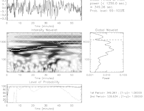
Figure 3: The wavelet result for H-alpha 6563 Å line near the loop foot point. The top panel shows the variation of intensity, the wavelet power spectrum is given in the middle panel, and the probability in the bottom panel. The light curve is from loop foot point (X,Y) = (58th pixel, 104th pixel), and smoothed by window width 60.

4 A Theoretical Interpretation

The intensity oscillation with the period of $P_{1}\approx$ 587 s likely represents the fundamental harmonic of either fast sausage (Nakariakov et al. 2003) or slow magnetoacoustic (Nakariakov et al. 2004) waves. The loop length is estimated as $L\approx$ 97 Mm with corresponding phase speed as $2L/P_{1}\sim$ 330 km/s. The estimated phase speed is much higher than the sound speed corresponding to cool H-alpha line. Therefore, we suggest that the oscillation is due to a fast sausage mode.

However, the dispersion relation of fast sausage waves in straight coronal loop includes both trapped and leaky modes depending on the loop parameters (Edwin & Roberts 1983; Nakariakov et al. 2003; Aschwanden et al. 2004). Due to low sound speed, we can easily use the cold plasma approximation. Hence, the cut-off wavenumber $k_{c}$ is (Edwin and Roberts 1983; Roberts et al. 1984)

$$k=k_{c}=\left[{v^{2}_{A}\over{v^{2}_{Ae}-v^{2}_{A}}}\right]^{1/2}{j_{0}\over a},$$ (1)

where $v_{A}$ and $v_{Ae}$ are Alfvén speeds inside and outside the loop, $a$ is the loop radius and $j_{0}=2.4$ is the first zero of the Bessel function $J_{0}$. The modes with $k>k_{c}$ are trapped in the loop, while the modes with $k<k_{c}$ are leaky. We may assume $B_{0}=B_{e}$, then the cut-off wavenumber is (Aschwanden et al. 2004)

$$k_{c}=\left[{1\over{{n_{0}/n_{e}}-1}}\right]^{1/2}{j_{0}\over a},$$ (2)

where $n_{0}/n_{e}$ is the electron density ratio inside and outside the loop. The width of selected loop can be roughly estimated as $2a\approx$ 6 Mm. Hence, the trapped global sausage mode can be realized only if the density ratio is

$${n_{0}\over n_{e}}>\left({j_{0}\over\pi}\right)^{2}\left({L\over a}\right)^{2}\approx 600.$$ (3)

Thus, only very dense loop can support non-leaky global sausage mode in the estimated length and width (Nakariakov et al. 2003; Aschwanden et al. 2004). The postflare loops usually have a very high density contrast of the order of $10^{2}$–$10^{3}$. The selected loop is cool post flare one, therefore the estimated density ratio falls in the expected range. Thus, the trapped sausage mode may occur in the loop, however, wave leakage can not be ruled out.

The fundamental harmonic of sausage oscillation has pressure antinode at the loop apex (upper panel in Fig. 4). Therefore, it modifies the density leading to the intensity oscillation. However, it has pressure node at the footpoints, and should not lead to remarkable intensity oscillation. The observations show strong oscillations at the loop apex with the period of $\approx$ 587 s and almost no indication of the oscillation with this period near foot point (see Fig. 2). Therefore, the oscillation with $\approx$ 587 s is probably due to the fundamental mode of sausage oscillations.

On the other hand, the first harmonic of sausage oscillation has pressure node at the loop apex and antinodes at the mid parts (lower panel in Fig. 4). Therefore, the first harmonic should show the intensity oscillation near the foot point and almost no oscillation at the loop apex (see Fig. 3). Indeed, the oscillation with the period of $\approx$ 349 s has high probability near foot point and no significant probability near the apex. Therefore, we interpret the oscillation with the period of $\approx$ 349 s as the first harmonic of fast sausage waves in the coronal loop. In the curved geometry, this mode is identical to sausage swaying mode (Díaz et al. 2006).

It must be mentioned that 349 s oscillation may be a consequence of nonlinear excitation from the fundamental harmonic, however, this possibility can be ruled out by two reasons: First, the amplitude of oscillation is not very strong and leaving a little space for nonlinear interaction; Secondly, the period of the first harmonic is not exactly twice of the period of fundamental mode, which was expected from the resonance condition.

Figure 4: The fundamental (upper panel) and its first (bottom panel) harmonics of sausage oscillations in coronal loops.

As a consequence of above discussions, we suggest for the first observational evidence of the fundamental and its first harmonics of fast sausage oscillations in cool postflare loop.

4.1 The period ratio $P_{1}/P_{2}$ of fundamental and first harmonics

The ratio between the periods of the fundamental and the first harmonics of sausage waves is proportional to $P_{1}/P_{2}\sim$ 1.68, which is significantly shifted from 2. Similar phenomena were observed for fast kink oscillations (Verwichte et al. 2004; De Moortel & Brady 2007; Van Doorsselaere et al. 2007). The deviation of $P_{1}/P_{2}$ from 2 in homogeneous loops is very small due to the wave dispersion (McEwan et al. 2006). But longitudinal density stratification causes significant shift of $P_{1}/P_{2}$ from 2 (Andries et al. 2005; McEwan et al. 2006; Van Doorsselaere et al. 2007).

Using the results of Andries et al. (2005), we estimate the density stratification along the loop as $L/\pi H\approx$ 1.8, where $H$ is the density scale height. The calculation of McEwan et al. (2006) gives the approximately same value. Thus, both calculation yields the same density scale height as $\sim$ 17 Mm for the loop length of 97 Mm.

It must be mentioned that seismologically estimated scale height of 17 Mm is larger comparing to the hydrostatical scale height at H-alpha temperature. This can be explained by two reasons: First, it is possible that the medium is not in equilibrium inside postflare loops; Second, some mechanism (e.g., the variation of loop cross section with height) other than the density stratification causes the deviation of $P_{1}/P_{2}$ from 2. Recently, Verth and Erdélyi (2008) have studied the effect of magnetic stratification on loop transverse kink oscillations and found that the loop divergence may have the significant effect on the period ratio almost similar to the density stratification. It would be interesting to study the effect of magnetic stratification on fast sausage oscillations. However, even if the loop divergence effect reduces the estimated scale height to $\sim$ 7-8 Mm, it still remains larger than equilibrium scale height. Therefore, we suggest that the post flare loops are not in equilibrium, which may cause plasma motions along the loop. In the movie of the observations, we clearly see the unidirectional mass motion from western foot point to eastern foot point in the selected loop which may indicate its departure from hydrostatic equilibrium. However, it will be interesting to search further the observational evidence in high resolution space data. The question is opened for further discussion.

4.2 Trapped or leaky mode?

It is not entirely clear from wavelet analysis that whether the global oscillation represents trapped or leaky mode. We see in Fig. 2 that the oscillation persists at least for 45 min, i.e., for $\sim$ 4-5 wave periods. However, the relative intensity plot in Fig. 2 (upper panel) likely shows that the oscillation amplitude decreases after 35 min. As intensity oscillations are due to the variation in plasma density, hence the decrement may reflect the process of wave damping. Since the oscillations are in sausage mode, the resonant absorption is unlikely to occur. Therefore, the wave leakage in the surroundings, is the most probable candidate for the wave damping. If the oscillation represents the global leaky mode instead of trapped one, then its phase speed would be close to the external Alfvén speed (Pascoe et al. 2007), which enables us to estimate its value as $v_{Ae}=2L/P_{1}\sim 330$ km/s. However this estimation is done for the straight magnetic cylinder, while noting that the curvature probably enhances the wave leakage (Verwichte et al. 2005; Díaz et al. 2006; Selwa et al. 2007).

For comparison, we may estimate the external Alfvén speed from the wave leakage in curved magnetic slab (Díaz et al. 2006). Using equation (25) of Díaz et al. (2006), we may write the expression for the external Alfvén speed as

$$v_{Ae}\sim{{2a}\over{\pi^{2}\tau_{d}}}{n_{0}\over n_{e}},$$

where $\tau_{d}$ is the damping time. From Fig. 2 , we estimate the damping time as

$$\tau_{d}\sim 20\,\,min,$$

then using the density ratio of $n_{0}/n_{e}\sim 600$ we estimate the value of the external Alfvén speed as $v_{Ae}\sim 300$ km/s (note, that this estimation is done for a curved slab, therefore Eq. (3), which is obtained for a straight loop, is not valid here).

5 Discussion and Conclusions

Using high spatial (1.3 arc sec) and temporal (5 and 10 s) resolution H-alpha observations, we found intensity oscillations with different periodicity in different parts of cool postflare loop. The intensity shows the oscillation with the period of $\approx$ 587 s at the loop apex and with the period of $\approx$ 349 s near loop footpoint. We interpret the oscillations as signature of the fundamental and first harmonics of fast sausage mode. It is difficult to say whether the oscillations are due to the trapped or leaky modes. However, intensity plot likely shows the decrement of the oscillation amplitude, therefore we suggest the presence of leaky nature of these modes. Seismologically estimated Alfvén speed outside the loop is $\sim$ 300-330 km/s. Using the period ratio $P_{1}/P_{2}$, we also estimate the density scale height in the loop as $\sim$ 17 Mm. This value is much higher than the equilibrium scale height at low H-alpha temperature, therefore we suggest that cool postflare loops are not in hydrostatic equilibrium. In the movie of the observations, we clearly see the unidirectional mass motion from western foot point to eastern foot point in the selected loop which indicates its departure from hydrostatic equilibrium.

In conclusions, we report the first observational evidence of multiple oscillations of fast sausage modes in cool chromospheric postflare loop. Future detailed observational search should be investigated, especially using recent space-based observations.

References

- andries (2005) Andries, J., Arregui, I. & Goossens, M., 2005, ApJ, 624, L57
- salman (2007) Ali, S.S., Uddin, W., Chandra, R., Mary, D.L. & Vrsnak, B., 2007, Sol. Phys., 240, 89
- Markus and Fletcher (1999) Aschwanden, M.J., Fletcher, L., Schrijver. C.J. & Alexander, D., 1999, ApJ, 520, 880
- Markus (2000) Aschwanden, M.J., Nightingale, R.W. & Alexander, D., 2000, ApJ, 541, 1059
- Markus (2004) Aschwanden, M.J., Nakariakov, V.M. & Melnikov, V.F., 2004, ApJ, 600, 458
- Inken and Brady (2007) De Moortel, I. & Brady, C.S., 2007, A&A, 664, 1210
- toni (2006) Díaz, A.J., Zaqarashvili, T.V. & Roberts, B., 2006, A&A, 455, 709
- bernie (1983) Edwin, P.M. & Roberts, B., 1983, Sol. Phys., 88, 179
- joshi (2003) Joshi, A., Chandra, Ramesh & Uddin, W., 2003, Sol. Phys., 217, 173
- mike (2006) McEwan, M.P., Donnelly, G.R., Díaz, A.J. & Roberts, B., 2006, A&A, 460, 893
- Valery and Leon (2001) Nakariakov, V.M. & Ofman, L., 2001, A&A, 372, L53
- Valery (2001) Nakariakov, V.M., Melnikov, V.F. & Reznikova, V.M., 2003, A&A, 412, L7
- Valery,David, andKelly (2001) Nakariakov, V.M., Tsiklauri, D., Kelly, A., Arber, T.D., Aschwanden, M.J., 2004, A&A, 414, L25
- Valery,Leon,DeLucaa, Roberts,and Joe (1999) Nakariakov, V.M., Ofman, L., DeLuca, E.E., Roberts, B. & Davila, J.M., 1999, Science, 285, 862
- Nemec and Nemec (1985) Linnell Nemec, A.F. & Nemec, J.M., 1985, Astronom J., 90, 2317
- Eoghan and Banerjee (2001) O’Shea, E., Banerjee, D., Doyle, J.G., Fleck, B. & Mugtagh, F., 2001, A&A, 368, 1095
- Eoghan and Srivastava (2007) O’Shea, E., Srivastava, A.K., Doyle, J.G. & Banerjee, D., 2007, A&A, 473, L13
- pascoe (2007b) Pascoe, D.J., Nakariakov, V.M. & Arber, T.D., 2007 a, A&A, 461, 1149
- sri (2008) Srivastava, A.K., Kuridze, D., Zaqarashvili, T.V., & Dwivedi, B.N., 2008, A&A, 481, L95
- Roberts (1984) Roberts, B., Edwin, P.M. & Benz, A .O., 1984, ApJ, 279, 857
- selwa (2007) Selwa, M., Murawski, K., Solanki, S. K. & Wang, T.J., 2007, A&A, 462, 1127
- Torrence and Compo (1998) Torrence, C. & Compo, G.P., 1998, BAMS, 79, 61
- tom (2007) Van Doorsselaere, T., Nakariakov, V.M. & Verwichte, E., 2007, A&A, 473, 959
- ervin1 (2005) Verwichte, E., Foullon, C. & Nakariakov, V.M., 2005, A&A, 446, 1139
- ervin (2007) Verwichte, E., Nakariakov, V.M., Ofman, L. & Deluca, E.E., 2004, Sol. Phys., 223, 77
- verth (2008) Verth, G. & Erdélyi, R., 2008, A&A (submitted)
- wang (2004) Wang, T.J. & Solanki, S., 2004, A&A, 421, L33