A novel method to construct stationary solutions of the Vlasov-Maxwell system : the relativistic case

Abstract

A method to derive stationary solutions of the relativistic Vlasov-Maxwell system is explored. In the non-relativistic case, a method using the Hermite polynomial series to describe the deviation from the Maxwell-Boltzmann distribution is found to be successful in deriving a few stationary solutions including two dimensional one. Instead of the Hermite polynomial series, two special orthogonal polynomial series, which are appropriate to expand the deviation from the Maxwell-Jüttner distribution, are introduced in this paper. By applying this method, a new two-dimensional equilibrium is derived, which may provide an initial setup for investigations of three-dimensional relativistic collisionless reconnection of magnetic fields.

I INTRODUCTION

Relativistic plasmas play important roles in high energy phenomena. In nature, gamma-ray burst afterglow is considered to be a phenomenon resulting from interaction of ultrarelativistic plasmas with a Lorentz factor $\gamma\simeq 10^{2}-10^{3}$ Shemi and Piran (1990); Paczynski (1990). Detailed observations of high energy astrophysical phenomena, such as supernova remnants, gamma-ray bursts, and active galactic nuclei, reveal that non-thermal components in their spectrum comprise of radiation from relativistic particles. In recent laser experiments, interaction of laser and plasmas is realized in highly relativistic regime. These phenomena often involve sufficiently rarefied plasma that the effect of collisions is negligible. In order to give plausible explanations for such phenomena, many authors have devoted their energies to investigations into properties of relativistic plasmas, i.e., instabilities, radiation, and stationary equilibria.

Here I propose a new method to obtain stationary equilibrium configurations of collisionless plasmas described by the relativistic Vlasov-Maxwell system. Such solutions are of great interest because they give self-consistent configurations of relativistic plasmas, which are used as an initial setup for studies on the relativistic collisionless reconnection of magnetic fields Parker (1957); Sweet (1956); Petschek (1964). In some recent numerical simulations of the relativistic collisionless magnetic reconnection Zenitani and Hoshino (2001); Jaroschek et al (2004), relativistic extensions of the harris sheet equilibrium Harris (1962) are used as the initial setup. While stationary solutions of the non-relativistic Vlasov-Maxwell system are well explored Harris (1962); Bennett (1934); Bernstein et al (1957); Mahajan (1989a, b); Attico and Pegoraro (1999); Bobrova et al (2001); Mottez (2003); Ceccherini et al (2005); Montagna and Pegoraro (2007), exploration of the relativistic Vlasov-Maxwell equilibria is not sufficient. Although Ref. Braasch (1997) discussed the existence of such solutions and derived a special class of them, studies on the derivation of the concrete expressions of the relativistic Vlasov-Maxwell equilibria are still rare.

In the previous paper Suzuki and Shigeyama (2008), a novel method to construct stationary solutions of the non-relativistic Vlasov-Maxwell system is proposed. In the method, the key concept is to describe the deviation of the distribution function from the Maxwell-Boltzmann by orthogonal polynomial series. The Hermite polynomial series is chosen for the purpose, because the weight function is Gaussian, which is equivalent to the Maxwell-Boltzmann distribution. Ref. Suzuki and Shigeyama (2008) reveals that this choice is appropriate to recover some well-known equilibria (the Harris sheet and the Bennet pinch) and derive a new equilibrium. In this paper, I will extend the previous method to deal with relativistic plasmas. Instead of the Maxwell-Boltzmann distribution, I use a relativistic extension of the Maxwell-Boltzmann distribution, i.e., the Maxwell-Jüttner distribution Juttner (1911) as the weight function of these polynomial series. To the best of my knowledge, there is no appropriate orthogonal polynomial series that describes the deviation from the Maxwell-Jüttner distribution as the Hermite polynomial does for non-relativistic plasmas. So I introduce two orthogonal polynomials in this paper. Applying the method, I can derive a new two-dimensional equilibrium, which is a relativistic extension of the equilibrium proposed in the previous paper. This equilibrium may provide an initial setup for numerical simulations of the relativistic collisionless reconnection.

This paper is organized as follows. In Sec.II, I describe the procedure of the method. In Sec.III, I apply the method to derive a stationary solution that I can treat it analytically. I conclude this paper in Sec.IV. Appendix gives some algebraic relations used in this paper.

II FORMULATION

The relativistic Vlasov equation describes the kinetic evolution of the distribution function $f_{j}(t,\mathbf{x},\mathbf{p})$ of particles $j$ ($=i$ for ions and $e$ for electrons) in the phase space $(x,y,z,p_{x},p_{y},p_{z})$ and the Maxwell equations describe the evolution of the electromagnetic fields. Here the cartesian coordinates in the real space are $(x,y,z)$ and the corresponding coordinates in the momentum space are $(p_{x},p_{y},p_{z})$. This system describes the exact behavior of relativistic collisionless plasmas. In this section, I derive stationary configuration of plasmas uniformly extending in the $z$ direction governed by the relativistic Vlasov-Maxwell system under the assumptions described in the following subsection.

II.1 Equations

Because physical variables do not depend on $t$ or $z$, the relativistic Vlasov equation is expressed as

$$\frac{p_{x}}{\sqrt{m_{j}^{2}c^{2}+|\mathbf{p}|^{2}}}\frac{\partial f_{j}}{\partial x}+\frac{p_{y}}{\sqrt{m_{j}^{2}c^{2}+|\mathbf{p}|^{2}}}\frac{\partial f_{j}}{\partial y}+\frac{q_{j}}{c}\left(E_{x}-\frac{p_{z}}{\sqrt{m_{j}^{2}c^{2}+|\mathbf{p}|^{2}}}B_{y}\right)\frac{\partial f_{j}}{\partial p_{x}}$$ (1)

$$\ \ \ +\frac{q_{j}}{c}\left(E_{y}+\frac{p_{z}}{\sqrt{m_{j}^{2}c^{2}+|\mathbf{p}|^{2}}}B_{x}\right)\frac{\partial f_{j}}{\partial p_{y}}+\frac{q_{j}}{c}\left(\frac{p_{x}}{\sqrt{m_{j}^{2}c^{2}+|\mathbf{p}|^{2}}}B_{y}-\frac{p_{y}}{\sqrt{m_{j}^{2}c^{2}+|\mathbf{p}|^{2}}}B_{x}\right)\frac{\partial f_{j}}{\partial p_{z}}=0,$$

where $f_{j}$ is the distribution function for particles $j$ with the charge $q_{j}$ and the mass $m_{j}$, $c$ is the speed of light and $|\mathbf{p}|=\sqrt{p_{x}^{2}+p_{y}^{2}+p_{z}^{2}}$ is the norm of the momentum. $E_{x},E_{y}$ and $B_{x},B_{y}$ represent the $x,y$-components of electric and magnetic fields, which are functions of $x$ and $y$. These electromagnetic fields are written as

$$E_{x}=-\frac{\partial\phi}{\partial x} E_{y}=-\frac{\partial\phi}{\partial y},$$ , (2a)

$$B_{x}=\frac{\partial A_{z}}{\partial y} B_{y}=-\frac{\partial A_{z}}{\partial x},$$ , (2b)

by introducing the scalar potential $\phi(x,y)$ and the $z$-component of the vector potential $A_{z}(x,y)$. The other components are assumed to vanish. These potentials satisfy the Poisson equations;

$$\frac{\partial^{2}\phi}{\partial x^{2}}+\frac{\partial^{2}\phi}{\partial y^{2}} = -4\pi\rho,$$ (3a)

$$\frac{\partial^{2}A_{z}}{\partial x^{2}}+\frac{\partial^{2}A_{z}}{\partial y^{2}} = -4\pi j_{z},$$ (3b)

where $\rho(x,y)$ and $j_{z}(x,y)$ are the charge density and the $z$-component of the electric current density, respectively. These are expressed in terms of $f_{j}(x,y,p_{x},p_{y},p_{z})$ as

$$\rho = \sum_{j}q_{j}\int^{\infty}_{-\infty}dp_{x}\int^{\infty}_{-\infty}dp_{y}\int^{\infty}_{-\infty}dp_{z}f_{j},$$ (4a)

$$j_{z} = \sum_{j}q_{j}\int^{\infty}_{-\infty}dp_{x}\int^{\infty}_{-\infty}dp_{y}\int^{\infty}_{-\infty}dp_{z}\frac{p_{z}}{\sqrt{m_{j}^{2}c^{2}+|\mathbf{p}|^{2}}}f_{j},$$ (4b)

which close the system. Solutions of Equations (1)-(4) give self-consistent configurations of collisionless plasmas.

II.2 Derivation of stationary solutions

In the following, I describe the procedure to derive solutions of Equations (1)-(4). The non-relativistic counterpart derived in the previous paper Suzuki and Shigeyama (2008) was based on the assumption that the deviation from the Maxwell-Boltzmann distribution can be expanded by the Hermite polynomial series. For a relativistic plasma, the distribution function in the thermodynamical equilibrium is given by the Maxwell-Jüttner distribution Juttner (1911), a relativistic extension of the classical Maxwell-Boltzmann distribution;

$$f^{\mathrm{MJ}}_{j}=\frac{n_{j}}{4\pi m_{j}^{2}ck_{\mathrm{B}}T_{j}K_{2}(\zeta_{j})}\exp\left[-\zeta_{j}\sqrt{1+\hat{p}_{x}^{2}+\hat{p}_{y}^{2}+\hat{p}_{z}^{2}}\right],$$ (5)

where $k_{\mathrm{B}}$ is the Boltzmann constant. $T_{j}$ and $n_{j}$ represents the temperature and the density of the particles $j$. I have assumed they are constant. $K_{2}(\zeta_{j})$ is the modified Bessel function of the second kind. Some dimensionless variables have been introduced as $\zeta_{j}=m_{j}c^{2}/(k_{\mathrm{B}}T_{j})$, $\hat{p}_{x}=p_{x}/(m_{j}c)$, $\hat{p}_{y}=p_{y}/(m_{j}c)$, and $\hat{p}_{z}=p_{z}/(m_{j}c)$.

In seeking solutions of Equations (1)-(4), I assume that the distribution function takes the following form;

$$f_{j}=\left\{\sum_{n=0}^{\infty}\left[g^{\mathrm{even}}_{j,n}(A_{z})S^{\mathrm{even}}_{n}(\hat{p}_{z})+g^{\mathrm{odd}}_{j,n}(A_{z})S^{\mathrm{odd}}_{n}(\hat{p}_{z})\right]\right\}\exp\left(-\frac{q_{j}\phi}{k_{\mathrm{B}}T_{j}}\right)f^{\mathrm{MJ}}_{j},$$ (6)

where $S_{n}^{\mathrm{even}}$ and $S_{n}^{\mathrm{odd}}$ are orthogonal polynomial series defined in Appendix B. Their coefficients $g_{j,n}^{\mathrm{even}}$ and $g_{j.n}^{\mathrm{odd}}$ are assumed to be functions of $A_{z}$. The distribution function in this form describes the deviation from the Maxwell-Jüttner distribution in terms of the orthogonal polynomial expansion. The spatial dependence of the distribution function is described through those of potentials $\phi$ and $A_{z}$. For large $\zeta_{j}$, these polynomials can be reduced to the Hermite polynomial series as

$$S^{\mathrm{even}}_{n}=\frac{H_{2n}(\sqrt{2\zeta}\hat{p}_{z})}{\zeta^{n}},\ \ \ S^{\mathrm{odd}}_{n}=\frac{H_{2n+1}(\sqrt{2\zeta}\hat{p}_{z})}{\zeta^{n+1/2}}.$$ (7)

Thus this method becomes equivalent to the previous method Suzuki and Shigeyama (2008) in the non-relativistic limit.

At first, substituting the expressions for fields (2) and the distribution function (6) into Equation (1), we obtain

$$\left\{\sum_{n=0}^{\infty}\left[\frac{dg_{j,n}^{\mathrm{even}}}{dA_{z}}S^{\mathrm{even}}_{n}(\hat{p}_{z})+\frac{dg_{j,n}^{\mathrm{odd}}}{dA_{z}}S^{\mathrm{odd}}_{n}(\hat{p}_{z})-\frac{q_{j}g_{j,n}^{\mathrm{even}}}{m_{j}c^{2}}\frac{dS_{n}^{\mathrm{even}}}{d\hat{p}_{z}}-\frac{q_{j}g_{j,n}^{\mathrm{odd}}}{m_{j}c^{2}}\frac{dS_{n}^{\mathrm{odd}}}{d\hat{p}_{z}}\right]\right\}f^{\mathrm{MJ}}_{j}=0$$ (8)

Then, to obtain equations to determine the coefficients $g^{\mathrm{even}}_{j,n}$ and $g^{\mathrm{odd}}_{j,n}$, both sides of this equation is multiplied by $S_{m}^{\mathrm{even}}(\hat{p}_{z})$ and integrated with respect to $\hat{p}_{x}$, $\hat{p}_{y}$, and $\hat{p}_{z}$. The orthogonality relation of $S^{\mathrm{even}}_{n}$ (38), the relation (47a), and the expression (49) yield the following ordinary differential equations,

$$\frac{dg^{\mathrm{even}}_{j,m}}{dA_{z}}-\frac{q_{j}}{m_{j}c^{2}}\sum_{k=m}^{\infty}B_{km}^{\mathrm{odd}}g^{\mathrm{odd}}_{j,k}=0.$$ (9)

On the other hand, multiplying both sides of Equation (8) by $S_{m}^{\mathrm{odd}}(\hat{p}_{z})/\sqrt{1+\hat{p}_{x}^{2}+\hat{p}_{y}^{2}+\hat{p}_{z}^{2}}$ and integrating with respect to $\hat{p}_{x}$, $\hat{p}_{y}$, and $\hat{p}_{z}$, other equations for coefficients

$$\frac{dg^{\mathrm{odd}}_{j,m}}{dA_{z}}-\frac{q_{j}}{m_{j}c^{2}}\sum_{k=m+1}^{\infty}B_{km}^{\mathrm{even}}g^{\mathrm{even}}_{j,k}=0,$$ (10)

are obtained. Here the relations (43) and (47b) have been used. Equations (9) and (10) give the relation between $g^{\mathrm{even}}_{j,n}$ and $g^{\mathrm{odd}}_{j,n}$. However, it is not practical to directly solve these infinite number of equations. Some restrictions are needed in order to solve them. For example, the condition $g^{\mathrm{even}}_{j,n}=g^{\mathrm{odd}}_{j,n}=0(n>N)$ or $g^{\mathrm{odd}}_{j,n}=g^{\mathrm{even}}_{j,n+1}=0(n>N)$, reduces Equations (9) and (10) to a finite number of ordinary differential equations and enable us to obtain expressions of $g^{\mathrm{even}}_{j,n}$ and $g^{\mathrm{odd}}_{j,n}$ as functions of $A_{z}$.

To derive the source terms in the Maxwell equations, substituting Equation (6) into Equations (4) and using the orthogonality relations (38), (43), and (47) again, these terms are written in terms of the potentials as

$$\rho = n_{i}q_{i}g_{i,0}^{\mathrm{even}}\exp\left(-\frac{q_{i}\phi}{k_{\mathrm{B}}T_{i}}\right)+n_{e}q_{e}g_{e,0}^{\mathrm{even}}\exp\left(-\frac{q_{e}\phi}{k_{\mathrm{B}}T_{e}}\right),$$ (11a)

$$j_{z} = \frac{n_{i}q_{i}}{\zeta_{i}}g^{\mathrm{odd}}_{i,0}\exp\left(-\frac{q_{i}\phi}{k_{\mathrm{B}}T_{i}}\right)+\frac{n_{e}q_{e}}{\zeta_{e}}g^{\mathrm{odd}}_{i,0}\exp\left(-\frac{q_{e}\phi}{k_{\mathrm{B}}T_{e}}\right),$$ (11b)

where the expressions (34) and (37) have been used for evaluation of integrals. Substitution of these expressions into Equations (3) leads to

$$\frac{\partial^{2}\phi}{\partial x^{2}}+\frac{\partial^{2}\phi}{\partial y^{2}} = -4\pi\left[n_{i}q_{i}g_{i,0}^{\mathrm{even}}\exp\left(-\frac{q_{i}\phi}{k_{\mathrm{B}}T_{i}}\right)+n_{e}q_{e}g_{e,0}^{\mathrm{even}}\exp\left(-\frac{q_{e}\phi}{k_{\mathrm{B}}T_{e}}\right)\right],$$ (12a)

$$\frac{\partial^{2}A_{z}}{\partial x^{2}}+\frac{\partial^{2}A_{z}}{\partial y^{2}} = -4\pi\left[\frac{n_{i}q_{i}}{\zeta_{i}}g^{\mathrm{odd}}_{i,0}\exp\left(-\frac{q_{i}\phi}{k_{\mathrm{B}}T_{i}}\right)+\frac{n_{e}q_{e}}{\zeta_{e}}g^{\mathrm{odd}}_{e,0}\exp\left(-\frac{q_{e}\phi}{k_{\mathrm{B}}T_{e}}\right)\right].$$ (12b)

Since $g^{\mathrm{even}}_{j,0}$ and $g^{\mathrm{odd}}_{j,0}$ are functions of $A_{z}$, these equations determine the potentials $\phi$ and $A_{z}$ as functions of $x$ and $y$ under certain boundary conditions.

As well as the previous method Suzuki and Shigeyama (2008), there is a limit in this method. For a stationary equilibrium, distribution functions can take various forms as long as the pressure balance is achieved. However, Equations (12) look as if there is a one-to-one correspondence between the field configuration and the distributions $g_{j,0}^{\mathrm{even}}$ and $g_{j,0}^{\mathrm{odd}}$. This disagreement arises from the assumption that the deviation of the distribution function from the Maxwell-Jüttner distribution can be expanded by the polynomial series $S^{\mathrm{even}}_{n}$ and $S^{\mathrm{odd}}_{n}$. Therefore, the stationary solutions derived above cover a part of many possible equilibria.

III Application

In this section, I consider an application of the stationary solutions derived above to a plasma in a charge neutrality comprising of electrons and ions with the same charge but the opposite sign ($q_{i}=-q_{e}=e$ and $n_{i}=n_{e}=n_{0}$) in which the electric field strength is sufficiently small ($\phi=0$). Then, Equation (12a) implies that ions and electrons have the same spatial distribution;

$$g^{\mathrm{even}}_{i,0}=g^{\mathrm{even}}_{e,0}.$$ (13)

As mentioned in the previous section, to solve Equations (9) and (10), I truncate both of the series as $g^{\mathrm{even}}_{j,n}=0(n\geq 2)$ and $g^{\mathrm{odd}}_{j,n}=0(n\geq 1)$. Then, Equations (9) and (10) reduce to the following three ordinary differential equations;

$$\frac{dg^{\mathrm{even}}_{j,0}}{dA_{z}}= \frac{q_{j}}{m_{j}c^{2}}g^{\mathrm{odd}}_{j,0},$$ (14)

$$\frac{dg^{\mathrm{odd}}_{j,0}}{dA_{z}}= \frac{2q_{j}}{m_{j}c^{2}}g^{\mathrm{even}}_{j,1},$$

$$\frac{dg^{\mathrm{even}}_{j,1}}{dA_{z}}= 0,$$

which have solutions in the form of

$$g^{\mathrm{even}}_{j,0}= g^{\mathrm{even}}_{j,1}(0)\left(\frac{q_{j}A_{z}}{m_{j}c^{2}}\right)^{2}+g^{\mathrm{odd}}_{j,0}(0)\frac{q_{j}A_{z}}{m_{j}c^{2}}+g^{\mathrm{even}}_{j,0}(0),$$ (15)

$$g^{\mathrm{odd}}_{j,0}= 2g^{\mathrm{even}}_{j,1}(0)\frac{q_{j}A_{z}}{m_{j}c^{2}}+g^{\mathrm{odd}}_{j,0}(0),$$

$$g^{\mathrm{even}}_{j,1}= g^{\mathrm{even}}_{j,1}(0),$$

where $g^{\mathrm{even}}_{j,0}(0)$, $g^{\mathrm{odd}}_{j,0}(0)$, and $g^{\mathrm{even}}_{j,1}(0)$ are constants of integration, which can take various values as long as the distribution function $f_{j}$ is positive at arbitrary points in the phase space and the condition (13) is satisfied. For example, I assume that they take the following values;

$$g^{\mathrm{even}}_{i,0}(0)=C,\ \ \ g^{\mathrm{odd}}_{i,0}(0)=0,\ \ \ g^{\mathrm{even}}_{i,1}(0)=1,$$ (16)

$$g^{\mathrm{even}}_{e,0}(0)=C,\ \ \ g^{\mathrm{odd}}_{e,0}(0)=0,\ \ \ g^{\mathrm{even}}_{e,1}(0)=\frac{m_{e}^{2}}{m_{i}^{2}},$$

where $C$ is a dimensionless constant. Some algebraic manipulations results in the distribution functions in the form of

$$f_{i} = \frac{n_{0}}{2\pi ck_{\mathrm{B}}T_{i}K_{2}(\zeta_{i})}\left[\frac{1}{m_{i}^{2}c^{2}}\left(p_{z}+\frac{eA_{z}}{c}\right)^{2}+C-\frac{K_{3}(\zeta_{i})}{\zeta_{i}K_{2}(\zeta_{i})}\right]$$ (17a)

$$\hskip 100.00015pt\times\exp\left[-\frac{c}{k_{\mathrm{B}}T_{i}}\sqrt{m_{i}^{2}c^{2}+p_{x}^{2}+p_{y}^{2}+p_{z}^{2}}\right],$$

$$f_{e} = \frac{n_{0}}{2\pi ck_{\mathrm{B}}T_{e}K_{2}(\zeta_{e})}\left[\frac{1}{m_{i}^{2}c^{2}}\left(p_{z}+\frac{eA_{z}}{c}\right)^{2}+C-\frac{m_{e}^{2}K_{3}(\zeta_{e})}{m_{i}^{2}\zeta_{e}K_{2}(\zeta_{e})}\right]$$ (17b)

$$\hskip 100.00015pt\times\exp\left[-\frac{c}{k_{\mathrm{B}}T_{e}}\sqrt{m_{e}^{2}c^{2}+p_{x}^{2}+p_{y}^{2}+p_{z}^{2}}\right].$$

These exactly satisfy the relativistic Vlasov equation (1). In order that the distribution function of ions $f_{i}$ takes positive values, the conditions

$$C\geq\frac{K_{3}(\zeta_{i})}{\zeta_{i}K_{2}(\zeta_{i})},\ \ \ C\geq\frac{m_{e}^{2}K_{3}(\zeta_{e})}{m_{i}^{2}\zeta_{e}K_{2}(\zeta_{e})}$$ (18)

are required.

Next, the equations governing the field configuration is deduced by substituting the solutions (15) and (16) into Equation (12b)

$$\frac{\partial^{2}A_{z}}{\partial x^{2}}+\frac{\partial^{2}A_{z}}{\partial y^{2}}=-\frac{8\pi e^{2}}{c^{2}}\left(\frac{n_{i}m_{i}}{\zeta_{i}}+\frac{n_{e}m_{e}}{\zeta_{e}}\right)A_{z}.$$ (19)

This equation has a solution in the form of

$$A_{z}=-B_{0}L\left[\cos(x/L)+\cos(y/L)\right],$$ (20)

where $L$ is a constant satisfying the following relation;

$$L=\frac{c}{2e}\sqrt{\frac{\zeta_{i}\zeta_{e}}{2\pi(n_{i}m_{i}\zeta_{e}+n_{e}m_{e}\zeta_{i})}}.$$ (21)

This vector potential generates a sinusoidal magnetic field as

$$B_{x}=B_{0}\sin(y/L),\ \ \ B_{y}=-B_{0}\sin(x/L).$$ (22)

Equations (17) and (20) provide a self-consistent configuration of relativistic plasmas. It is found that this equilibrium is a relativistic extension of the equilibrium proposed in the previous paper Suzuki and Shigeyama (2008).

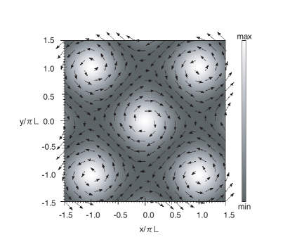
Figure 1: The configuration of the two-dimensional relativistic Vlasov-Maxwell equilibrium derived by applying the method in this paper. The gray scale represents the density distribution of electrons (or ions) in arbitrary units and the arrows represent the magnetic fields.

Figure 1 illustrates the thus derived configuration of equilibrium. The gray scale and the arrows represent the density distribution $g_{j,0}^{\mathrm{even}}$ of electrons or ions in arbitrary units and the magnetic field, respectively. As in the non-relativistic counterpart Suzuki and Shigeyama (2008), we can see that the current filaments lie along the $z$-axis and generate the magnetic fields around themselves. Each filament is surrounded by four filaments that carry anti-parallel currents.

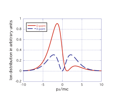
Figure 2: (Color online) The momentum distributions of ions at the O-point (solid line) and the X-point (dashed line).

Here, I focus on the momentum distributions at two points. One is the center of a filament (referred to as the O-point) and the other is a middle point between the filaments carrying parallel currents (referred to as the X-point). The magnetic field at the X-point is sheared like the Harris sheet equilibrium. Figure 2 shows the momentum distributions of ions at the X and O-points. The values of parameters are as follows; $B_{0}=0.1m_{e}\omega_{e}/e$, where $\omega_{e}$ is the electron plasma frequency, and $kT_{i}=kT_{e}=m_{i}c^{2}$. From these values, one obtains

$$\frac{K_{3}(\zeta_{i})}{\zeta_{i}K_{2}(\zeta_{i})}\simeq 0.0005,\ \ \ \frac{m_{e}^{2}K_{3}(\zeta_{e})}{m_{i}^{2}\zeta_{e}K_{2}(\zeta_{e})}\simeq 0.$$ (23)

So I have assumed $C=0.0005$. While a symmetric double-peak distribution appears at the X-point due to $A_{z}=0$, an asymmetric one is achieved at the O-point.

In contrast to ions, the momentum distribution of electrons has a symmetric double-peak both at the X and O-points, because the term $e^{2}A_{z}^{2}/m_{i}^{2}c^{4}(<0.04m_{e}^{2}\omega_{e}^{2}L^{2}/m_{i}^{2}c^{4})$ is much smaller than $C(=0.0005)$.

Finally, I make a remark on one of the relativistic effects. In comparison with the non-relativistic counterpart, the distribution tends to have a relatively shallow slope in the high-energy regime, which comes from the difference in the equilibrium distribution. While the Maxwell-Boltzmann distribution is proportional to $\exp(-p_{z}^{2}/2m_{j}k_{\mathrm{B}}T)$, the Maxwell-Jüttner distribution is proportional to $\exp(-cp_{z}/k_{\mathrm{B}}T)$ in the limit of $p_{z}/m_{j}c\gg 1$. In other words, the relativistic one has more high-energy particles than the non-relativistic does.

IV CONCLUSIONS

In this paper, I have developed a novel method to construct stationary solutions of the relativistic Vlasov-Maxwell system. By applying the method, a new two-dimensional equilibrium, which is a relativistic extension of the previous work Suzuki and Shigeyama (2008), is proposed. A comparison of the non-relativistic and the relativistic equilibrium is done. As well as the non-relativistic equilibrium, a sheared magnetic field is generated in the relativistic one. On the other hand, they show different behaviors in the high-energy regime. It may provide an initial setup for investigations of the relativistic collisionless magnetic reconnection that takes into account three-dimensional effects. It will be intriguing to investigate the stability of the equilibrium derived in this paper.

Appendix A Properties of the Modified Bessel Functions of Second Kind

In the next section, I often use the properties of the modified Bessel functions of second kind. Therefore, I review the properties in this section Gray and Mathews (1922).

The $n$th-order modified Bessel functions of second kind $K_{n}(x)$ is defined by the following integral;

$$K_{n}(x)=\int^{\infty}_{0}e^{-x\cosh\theta}\cosh(n\theta)d\theta.$$ (24)

It is known that $K_{n}(x)$ and $K_{n+1}$ satisfy the following recurrence formula;

$$\frac{d}{dx}\left(\frac{K_{n}}{x^{n}}\right)=-\frac{K_{n+1}}{x^{n}}.$$ (25)

After some algebraic manipulations, $K_{n}(x)$ is expressed in another form as

$$K_{n}(x)=\left(\frac{x}{2}\right)^{n}\frac{\Gamma(1/2)}{\Gamma(n+1/2)}\int^{\infty}_{0}e^{-x\cosh t}\sinh^{2n}tdt.$$ (26)

Dividing both sides of this equation by $x^{n}$ and differentiating with respect to $x$ yields the relation

$$K_{n+1}(x)=\left(\frac{x}{2}\right)^{n}\frac{\Gamma(1/2)}{\Gamma(n+1/2)}\int^{\infty}_{0}e^{-x\cosh t}\cosh t\sinh^{2n}tdt.$$ (27)

In the limit of $x\gg 1$, $K_{n}(x)$ reduces to

$$K_{n}(x)\simeq\sqrt{\frac{\pi}{2x}}e^{-x}.$$ (28)

Appendix B Construction fo Orthogonal Polynomials

In this section, I construct two special orthogonal polynomial series used in this paper.

B.1 Some useful integrals

In constructing the polynomials, two integrals are used again and again. These integrals are introduced beforehand.

The first one is

$$I_{n}^{\mathrm{odd}}=\int^{\infty}_{-\infty}\int^{\infty}_{-\infty}\int^{\infty}_{-\infty}\hat{p}_{z}^{2n}\exp\left[-\zeta\sqrt{1+\hat{p}_{x}^{2}+\hat{p}_{y}^{2}+\hat{p}_{z}^{2}}\right]\frac{d\hat{p}_{x}d\hat{p}_{y}\hat{p}_{z}}{\sqrt{1+\hat{p}_{x}^{2}+\hat{p}_{y}^{2}+\hat{p}_{z}^{2}}}.$$ (29)

where $n$ is an integer and $\zeta$ is an independent variable. Introducing the spherical coordinates $(p,\theta,\phi)$ as

$$\hat{p}_{x}=p\sin\theta\cos\phi,\ \ \ \hat{p}_{y}=p\sin\theta\sin\phi,\ \ \ \hat{p}_{z}=p\cos\theta,$$ (30)

the integrations with respect to $\theta$ and $\phi$ can be performed to obtain

$$I_{n}^{\mathrm{odd}}=\frac{4\pi}{2n+1}\int^{\infty}_{0}p^{2n+2}\exp\left[-\zeta\sqrt{1+p^{2}}\right]\frac{dp}{\sqrt{1+p^{2}}}.$$ (31)

Furthermore, a change of the integral variable from $p$ to $t$ defined as

$$p=\sinh t,$$ (32)

leads to

$$I_{n}^{\mathrm{odd}}=\frac{4\pi}{2n+1}\int^{\infty}_{0}e^{-\zeta\cosh t}\sinh^{2n+2}tdt.$$ (33)

Using the relation (26), the integral is expressed in terms of $K_{n+1}$ as

$$I_{n}^{\mathrm{odd}}=\frac{2^{n+2}\pi\Gamma(n+1/2)}{\zeta^{n+1}\Gamma(1/2)}K_{n+1}(\zeta)$$ (34)

The second integral is

$$I_{n}^{\mathrm{even}}=\int^{\infty}_{-\infty}\int^{\infty}_{-\infty}\int^{\infty}_{-\infty}\hat{p}_{z}^{2n}\exp\left[-\zeta\sqrt{1+\hat{p}_{x}^{2}+\hat{p}_{y}^{2}+\hat{p}_{z}^{2}}\right]d\hat{p}_{x}d\hat{p}_{y}d\hat{p}_{z}.$$ (35)

Again, from the relations (30) and (32), this integral is converted to

$$I_{n}^{\mathrm{even}}=\frac{4\pi}{2n+1}\int^{\infty}_{0}e^{-\zeta\cosh t}\sinh^{2n+2}t\cosh tdt$$ (36)

Using the relation (27), the integral is expressed in terms of $K_{n+2}$ as

$$I_{n}^{\mathrm{even}}=\frac{2^{n+2}\pi\Gamma(n+1/2)}{\zeta^{n+1}\Gamma(1/2)}K_{n+2}(\zeta)$$ (37)

B.2 Even orthogonal polynomials

I construct the polynomial series $S^{\mathrm{even}}_{n}(\hat{p}_{Z})$. This polynomial must satisfy two conditions; (1) These are even functions. (2) The set $S^{\mathrm{even}}_{n}$ forms an orthogonal basis in the even function space, in other words, each polynomials satisfy the following orthogonality relation,

$$\int^{\infty}_{-\infty}\int^{\infty}_{-\infty}\int^{\infty}_{-\infty}S^{\mathrm{even}}_{m}(\hat{p_{z}})S^{\mathrm{even}}_{n}(\hat{p_{z}})\exp\left[-\zeta\sqrt{1+\hat{p}_{x}^{2}+\hat{p}_{y}^{2}+\hat{p}_{z}^{2}}\right]d\hat{p}_{x}d\hat{p}_{y}d\hat{p}_{z}\propto\delta_{mn},$$ (38)

where I choose $\exp\left[-\zeta\sqrt{1+\hat{p}_{x}^{2}+\hat{p}_{y}^{2}+\hat{p}_{z}^{2}}\right]$ as the weight function and $\delta_{mn}$ represents Kronecker’s delta. Then we define the polynomials $S^{\mathrm{even}}_{n}$ as

$$S^{\mathrm{even}}_{0}=1,\ \ \ S^{\mathrm{even}}_{n}=\hat{p}_{z}^{2n}+\sum_{k=0}^{n-1}A_{nk}^{\mathrm{even}}S^{\mathrm{even}}_{k},$$ (39)

where $A_{nk}^{\mathrm{even}}$ are coefficients determined by the orthogonality relation (38). Multiplying $S^{\mathrm{even}}_{n}$ in (39) by $S^{\mathrm{even}}_{m}\exp\left[-\zeta\sqrt{1+\hat{p}_{x}^{2}+\hat{p}_{y}^{2}+\hat{p}_{z}^{2}}\right](m<n)$ and integrating it with respect to $\hat{p}_{x}$, $\hat{p}_{y}$, and $\hat{p}_{z}$, the following expression for $A^{\mathrm{even}}_{nk}$ is obtained;

$$A_{nm}^{\mathrm{even}}=-\frac{\int^{\infty}_{-\infty}\int^{\infty}_{-\infty}\int^{\infty}_{-\infty}\hat{p}_{z}^{2n}S^{\mathrm{even}}_{m}\exp\left[-\zeta\sqrt{1+\hat{p}_{x}^{2}+\hat{p}_{y}^{2}+\hat{p}_{z}^{2}}\right]d\hat{p}_{x}d\hat{p}_{y}d\hat{p}_{z}}{\int^{\infty}_{-\infty}\int^{\infty}_{-\infty}\int^{\infty}_{-\infty}(S^{\mathrm{even}}_{m})^{2}\exp\left[-\zeta\sqrt{1+\hat{p}_{x}^{2}+\hat{p}_{y}^{2}+\hat{p}_{z}^{2}}\right]d\hat{p}_{x}d\hat{p}_{y}d\hat{p}_{z}}.$$ (40)

Using this equation, one can determine the $n$th order polynomial $S^{\mathrm{even}}_{n}$ by induction. For example, the denominator and numerator of $A_{10}^{\mathrm{even}}$ become $I^{\mathrm{even}}_{0}$ and $I^{\mathrm{even}}_{1}$, respectively. Thus $A_{10}^{\mathrm{even}}(=S^{\mathrm{even}}-\hat{p}_{z}^{2})$ is expressed as

$$A_{10}^{\mathrm{even}}=-\frac{K_{3}(\zeta)}{\zeta K_{2}(\zeta)}.$$ (41)

In such a way, the even polynomials $S^{\mathrm{even}}_{n}$ are obtained from the lower order polynomials $S^{\mathrm{even}}_{m}(m<n)$. The expression of the first three are

$$S^{\mathrm{even}}_{0} = 1,$$ (42a)

$$S^{\mathrm{even}}_{1} = \hat{p}_{z}^{2}-\frac{K_{3}(\zeta)}{\zeta K_{2}(\zeta)},$$ (42b)

$$S^{\mathrm{even}}_{2} = \hat{p}_{z}^{4}-\frac{3}{\zeta}\frac{5K_{5}(\zeta)K_{2}(\zeta)-K_{4}(\zeta)K_{3}(\zeta)}{3K_{4}(\zeta)K_{2}(\zeta)-[K_{3}(\zeta)]^{2}}\left[\hat{p}_{z}^{2}-\frac{K_{3}(\zeta)}{\zeta K_{2}(\zeta)}\right]-\frac{3K_{4}(\zeta)}{\zeta^{2}K_{2}(\zeta)}.$$ (42c)

B.3 Odd orthogonal polynomials

The odd polynomial series $S^{\mathrm{odd}}_{n}(\hat{p}_{z})$ are supposed to satisfy the following orthogonal relation,

$$\int^{\infty}_{-\infty}\int^{\infty}_{-\infty}\int^{\infty}_{-\infty}S^{\mathrm{odd}}_{m}(\hat{p_{z}})S^{\mathrm{odd}}_{n}(\hat{p_{z}})\exp\left[-\zeta\sqrt{1+\hat{p}_{x}^{2}+\hat{p}_{y}^{2}+\hat{p}_{z}^{2}}\right]\frac{d\hat{p}_{x}d\hat{p}_{y}d\hat{p}_{z}}{\sqrt{1+\hat{p}_{x}^{2}+\hat{p}_{y}^{2}+\hat{p}_{z}^{2}}}\propto\delta_{mn}.$$ (43)

Note that the weight function differs from that of the even polynomial series. Then I define the polynomials $S^{\mathrm{odd}}_{n}$ as

$$S^{\mathrm{odd}}_{0}=\hat{p}_{z},\ \ \ S^{\mathrm{odd}}_{n}=\hat{p}_{z}^{2n+1}+\sum_{k=0}^{n-1}A_{nk}^{\mathrm{odd}}S^{\mathrm{odd}}_{k},$$ (44)

where $A^{\mathrm{odd}}_{nk}$ are coefficients determined by the same procedure as the even polynomial series. Thus, $A^{\mathrm{odd}}_{nm}$ are expressed as

$$A^{\mathrm{odd}}_{nm}=-\frac{\int^{\infty}_{-\infty}\int^{\infty}_{-\infty}\int^{\infty}_{-\infty}\hat{p}_{z}^{2n+1}S^{\mathrm{odd}}_{m}\exp\left[-\zeta\sqrt{1+\hat{p}_{x}^{2}+\hat{p}_{y}^{2}+\hat{p}_{z}^{2}}\right]d\hat{p}_{x}d\hat{p}_{y}d\hat{p}_{z}}{\int^{\infty}_{-\infty}\int^{\infty}_{-\infty}\int^{\infty}_{-\infty}(S^{\mathrm{odd}}_{m})^{2}\exp\left[-\zeta\sqrt{1+\hat{p}_{x}^{2}+\hat{p}_{y}^{2}+\hat{p}_{z}^{2}}\right]d\hat{p}_{x}d\hat{p}_{y}d\hat{p}_{z}}.$$ (45)

From this equation and the relation (34), one can derive the expression of the odd polynomial series. The first three are

$$S^{\mathrm{odd}}_{0} = \hat{p}_{z},$$ (46a)

$$S^{\mathrm{odd}}_{1} = \hat{p}_{z}^{3}-\frac{3K_{3}(\zeta)}{\zeta K_{2}(\zeta)}\hat{p}_{z},$$ (46b)

$$S^{\mathrm{odd}}_{2} = \hat{p}_{z}^{5}-\frac{5}{\zeta}\frac{7K_{5}(\zeta)K_{2}(\zeta)-3K_{4}(\zeta)K_{3}(\zeta)}{5K_{4}(\zeta)K_{2}(\zeta)-3[K_{3}(\zeta)]^{2}}\left[\hat{p}_{z}^{3}-\frac{3K_{3}(\zeta)}{\zeta K_{2}(\zeta)}\hat{p}_{z}\right]-\frac{15K_{4}(\zeta)}{\zeta^{2}K_{2}(\zeta)}\hat{p}_{z}.$$ (46c)

B.4 Properties

Here I list some properties of the two orthogonal polynomial series derived above. Because the products $S^{\mathrm{even}}_{n}S^{\mathrm{odd}}_{m}$ are odd function with respect to $\hat{p}_{z}$, the following integrals vanish;

$$\int^{\infty}_{-\infty}\int^{\infty}_{-\infty}\int^{\infty}_{-\infty}S^{\mathrm{even}}_{n}S^{\mathrm{odd}}_{m}\exp\left[-\zeta\sqrt{1+\hat{p}_{x}^{2}+\hat{p}_{y}^{2}+\hat{p}_{z}^{2}}\right]d\hat{p}_{x}d\hat{p}_{y}d\hat{p}_{z} = 0,$$ (47a)

$$\int^{\infty}_{-\infty}\int^{\infty}_{-\infty}\int^{\infty}_{-\infty}S^{\mathrm{even}}_{n}S^{\mathrm{odd}}_{m}\exp\left[-\zeta\sqrt{1+\hat{p}_{x}^{2}+\hat{p}_{y}^{2}+\hat{p}_{z}^{2}}\right]\frac{d\hat{p}_{x}d\hat{p}_{y}d\hat{p}_{z}}{\sqrt{1+\hat{p}_{x}^{2}+\hat{p}_{y}^{2}+\hat{p}_{z}^{2}}} = 0.$$ (47b)

Next, the derivatives of the polynomials can be expanded by $S^{\mathrm{odd}}_{n}$;

$$\frac{dS^{\mathrm{even}}_{n}}{d\hat{p}_{z}}=\sum_{k=0}^{n-1}B^{\mathrm{even}}_{nk}S^{\mathrm{odd}}_{k}.$$ (48)

Because the derivatives of $S^{\mathrm{even}}_{n}$ is an odd function. On the other hand, the derivatives of $S^{\mathrm{odd}}_{n}$ can be expanded by $S^{\mathrm{even}}_{n}$;

$$\frac{dS^{\mathrm{odd}}_{n}}{d\hat{p}_{z}}=\sum_{k=0}^{n}B^{\mathrm{odd}}_{nk}S^{\mathrm{even}}_{k}.$$ (49)

The expressions of $B^{\mathrm{even}}_{nk}$ and $B^{\mathrm{odd}}_{nk}$ are obtained by directly differentiating the expressions (42), (46), and their extensions for larger $n$.

References

- Shemi and Piran (1990) A. Shemi, and T. Piran, Astrophys. J. Lett., 365, L55 (1990).
- Paczynski (1990) B. Paczynski, Astrophys. J., 424, 708 (1990).
- Cercignani and Kremer (2002) C. Cercignani, and G. M. Kremer, The Relativistic Boltzmann Equation: Theory and Applications (Birkhauser, Boston, 2002) p.31.
- Parker (1957) E. N. Parker, Phys. Rev., 107, 830 (1957).
- Sweet (1956) P. A. Sweet, ”The neutral point theory of solar flares,” in Electromagnetic Phenomena in Cosmical Physics, edited by B. Lehnert (Cambridge University Press, 1958) p.123.
- Petschek (1964) H. E. Petschek, ”Magnetic field annihilation” in Physics of Solar Flares, edited by W. N. Ness, NASA SP-50, p.425 (1964).
- Zenitani and Hoshino (2001) S. Zenitani, and M. Hoshino, Astrophys. J. Lett. 562 L62 (2001).
- Jaroschek et al (2004) C. H. Jaroschek, R. A. Treumann, H. Lesch, and M. Scholer, Phys. Plasmas 11, 1151 (2004).
- Harris (1962) E. G. Harris, Nuovo Cimento 23, 115 (1962).
- Bennett (1934) D. Bennett, Phys. Rev. 45, 890 (1934).
- Bernstein et al (1957) B. Bernstein, J. M. Greene, and M. D. Kruskal, Phys. Rev. 108, 546 (1957).
- Mahajan (1989a) S. M. Mahajan, Phys. Fluids B, 1, 43 (1989).
- Mahajan (1989b) S. M. Mahajan, and W.-Q. Li, Phys. Fluids B 1, 2345 (1989).
- Attico and Pegoraro (1999) N. Attico, and F. Pegoraro, Phys. Plasmas 6, 767 (1999).
- Bobrova et al (2001) N. A. Bobrova and S. V. Bulanov, J. I. Sakai, and D. Sugiyama, Phys. Plasmas 8, 759 (2001).
- Mottez (2003) F. Mottez, Phys. Plasmas 10, 2501 (2003).
- Ceccherini et al (2005) F. Ceccherini, C. Montagna, F. Pegoraro, and G. Cicogna, Phys. Plasmas 12, 052506 (2005).
- Montagna and Pegoraro (2007) C. Montagna, and F. Pegoraro, Phys. Plasmas 14, 042103 (2007).
- Braasch (1997) P. Braasch, Math. Meth. Appl. Sci. 20, 667 (1997).
- Suzuki and Shigeyama (2008) A. Suzuki, and T. Shigeyama, Phys. Plasmas 15, 042107 (2008).
- Juttner (1911) F. Juttner, Ann. Phys. 34, 856 (1911).
- Gray and Mathews (1922) A. Gray and G. B. Mathews, A treatise on Bessel functions and their applications to physics, (Macmillan, London, 1922).