In-situ generation of transverse MHD waves from colliding flows in the solar corona

Abstract

Transverse MHD waves permeate the solar atmosphere and are a candidate for coronal heating. However, the origin of these waves is still unclear. In this work, we analyse coordinated observations from Hinode/SOT and IRIS of a prominence/coronal rain loop-like structure at the limb of the Sun. Cool and dense downflows and upflows are observed along the structure. A collision between a downward and an upward flow with an estimated energy flux of $10^{7}-10^{8}$ erg cm^-2 s^-1 is observed to generate oscillatory transverse perturbations of the strands with an estimated $\approx 40~{}$km s^-1 total amplitude, and a short-lived brightening event with the plasma temperature increasing to at least $10^{5}~{}$K. We interpret this response as sausage and kink transverse MHD waves based on 2D MHD simulations of plasma flow collision. The lengths, density and velocity differences between the colliding clumps and the strength of the magnetic field are major parameters defining the response to the collision. The presence of asymmetry between the clumps (angle of impact surface and/or offset of flowing axis) is crucial to generate a kink mode. Using the observed values we successfully reproduce the observed transverse perturbations and brightening, and show adiabatic heating to coronal temperatures. The numerical modelling indicates that the plasma $\beta$ in this loop-like structure is confined between $0.09$ and $0.36$. These results suggest that such collisions from counter-streaming flows can be a source of in-situ transverse MHD waves, and that for cool and dense prominence conditions such waves could have significant amplitudes.

1 Introduction

Transverse MHD waves permeate the solar atmosphere and constitute a possible candidate for coronal heating (for a review, see for example Arregui et al., 2012; De Moortel & Nakariakov, 2012; Arregui, 2015). A main source of evidence of these waves comes from observations of prominences and coronal rain, in which the naturally cold, dense and optically thicker plasma conditions allow much higher spatial resolution and reduced line-of-sight confusion (Lin et al., 2005; Lin, 2011; Okamoto et al., 2007; Ning et al., 2009; Hillier et al., 2013; Schmieder et al., 2013; Okamoto et al., 2015; Vial & Engvold, 2015). However, the origin of these waves (in coronal and prominence structures) remains unclear and is usually assumed to be in convective motions, or through mode conversion of $p-$modes propagating from the solar interior.

Another commonly observed feature of cool coronal structures such as prominences and rainy loops are field-aligned flows with speeds of $10-100$ km s^-1 and $40-200$ km s^-1, respectively (Ofman & Wang, 2008; Antolin & Rouppe van der Voort, 2012; Alexander et al., 2013; Kleint et al., 2014). Both downflows and upflows are observed along the legs of prominences (Vial & Engvold, 2015). These longitudinal dynamics are commonly associated to the formation mechanism of prominences or coronal rain, such as thermal instability or thermal non-equilibrium (Antiochos et al., 1999; Karpen et al., 2001; Antolin et al., 2010; Xia et al., 2017).

Through coordinated observations of a prominence/coronal rain complex (§2) with Hinode (Kosugi et al., 2007), the Interface Region Imaging Spectrograph (IRIS; De Pontieu et al., 2014) and the Solar Dynamics Observatory(SDO; Pesnell et al., 2012), and numerical MHD modelling (§4), we show that in-situ collisions from such counter-streaming flows could be a source of transverse MHD waves in the corona.

2 Observations

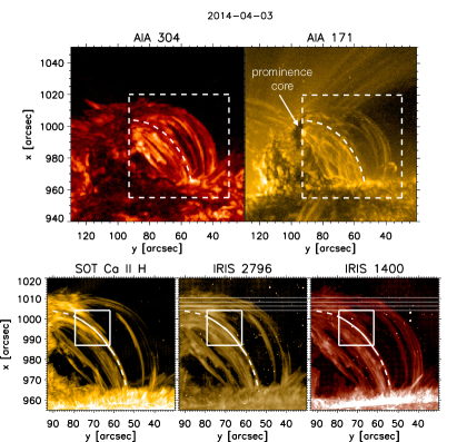
Figure 1: From top left to bottom right we show variance images (sum of squared differences from a 8 min average image) in the AIA 304, AIA 171, in the SOT Ca II H, SJI 2796 and SJI 1400 of IRIS. The FOV of the bottom three panels is shown as a dashed square in the top 2 panels. A particular set of downflows is followed along one of these structures (white dashed/solid curve). The horizontal dotted lines in the IRIS panels indicate the location of the slit during the 4-step raster. Note that the solar East-West direction corresponds to the vertical axes in the panels.

On April 3rd, 2014, SDO, IRIS and Hinode co-observed a prominence/coronal rain complex on the West limb of the Sun (IRIS-Hinode operation plan 254), shown in Fig. 1. The Hinode Solar Optical Telescope (SOT; Suematsu et al., 2008; Tsuneta et al., 2008) observed from 13:16UT to 14:30UT in the Ca II H line, with a cadence of 8 s (1.23 s exposure), with $0.^{\prime\prime}109$ pixel^-1 platescale, and a field-of-view (FOV) of $111\arcsec\times 111\arcsec$, centred at helioprojective coordinates $(x,y)=(996.5,31.1)$. IRIS observed from 13:16UT to 14:53UT with a 4-step sparse raster program (OBS ID 3840259471), with a cadence for the Slit-Jaw Imager (SJI) of 18.27 s (exposure time of 8 s) and 9 s for the spectrograph SG (roughly 37 s per raster position), with $0.^{\prime\prime}166$ pixel^-1 platescale, a FOV of $127\arcsec\times 128\arcsec$ centred at $(x,y)=(1007.1,34.2)$, containing the SOT FOV. The IRIS observing program included both the SJI 2796 and SJI 1400 filtergrams, which are dominated by Mg II k emission at 2796.35 Å around $2\times 10^{4}$ K and Si IV emission at 1402.77 Å around $10^{5}~{}$K, respectively. The images from the Atmospheric Imaging Assembly (AIA; Lemen et al., 2011) were in level 1.5. Their cadence is $12~{}$s, with a platescale of $0.^{\prime\prime}6$ pixel^-1.

The SOT dataset was processed using the $\tt{FG\_PREP}$ Solarsoft routine. The SJI data corresponds to level 2 data (De Pontieu et al., 2014), which includes correction for thermal variations of the pointing by co-aligning each image using a cross correlation maximisation routine. SOT, IRIS and AIA data were co-aligned manually.

The target of the observations was a loop-like structure stemming from a high ($\approx 55\arcsec$ above the limb) prominence core, reminiscent of the model by Keppens & Xia (2014). In Fig. 1 we show a variance image of this structure in Ca II H, SJI 2796 and SJI 1400, where the variance is taken over the first 8 min of the observation.

3 Colliding flows

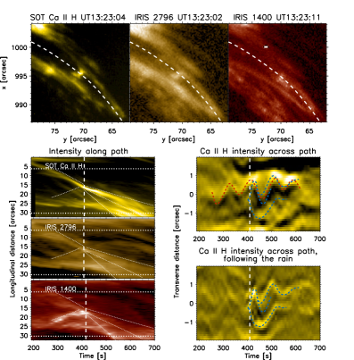
Figure 2: The 3 top panels show, from left to right, the region indicated by the small white square (solid lines) of Fig. 1, in the Ca II H line of SOT, the SJI 2796 and SJI 1400 of IRIS. The white dashed curve shows the path of counter-streaming plasma clumps. The time-distance diagram along this path is shown in the 3 left panels, where distance is measured from the top of the path shown in Fig. 1. The intensity is integrated over a width of $1\arcsec$. The horizontal dotted lines in these panels indicate the top and bottom coordinates along the trajectory within the FOV of the top 3 panels. The vertical dashed line indicates the closest time to collision for each channel. The middle and bottom right panels show transverse cuts to the trajectory of the clumps. The contours of the brightest oscillatory paths are traced visually in dashed red and blue curves, respectively for the middle and bottom right panels. In the middle panel the intensity along part of the path (solid curve in Fig. 1) is integrated for each transverse cut. In the lower panel the downflowing set of clumps is followed and at each time the transverse cut to the trajectory is plotted. See also the accompanying animation.

The focus of the present investigation is the main loop-like structure connected to the prominence core seen in the middle of the images in Fig. 1. The flows along this loop structure are clumpy and multi-stranded, particularly in the higher resolution Ca II H intensity images, a general characteristic of coronal rain material when observed at high resolution (Antolin et al., 2015). Mostly downflows are observed, stemming from the prominence core (top left) towards the surface. Additionally, and in contrast to the usual coronal rain, the current case also exhibits a significant amount of upflows probably caused by dips at the loop apex, enhancing thermal instability.

We follow a particular set of clumps during their downward trajectory (dashed curve in Figs. 1 and 2) at a constant velocity of $\approx 50$ km s^-1 in the plane-of-the-sky (POS). At high resolution in Ca II H, the clumps are $0.3\arcsec-1.4\arcsec$ in width (across the loop), with a continuously variable length of a few arcsec. Half-way along the loop at $t=13.23$UT the clumps’ intensities in all 3 channels suddenly increase, and a bright front of about $2\arcsec$ in width is observed (visible in Fig. 2). Afterwards, the downward speeds of some of the clumps are reduced by half, as seen in the time-distance diagram along the loop (3-set bottom left panels in Fig. 2). In addition, the clumps are seen to oscillate transversely in Ca II H following the intensity increase. This is best seen in the time-distance diagram transverse to the loop (bottom right panel in Fig. 2), where we follow the clump along its downward trajectory. We can see that some clumps undergo an outward transverse motion of $\approx 1\arcsec$ (radially away from the Sun, positive transverse distance in the panel), while others undergo an inwards transverse motion of similar amplitude. The initial transverse velocity in the POS is $\approx 25$ km s^-1. The outward transverse motion can be tracked for longer times and the oscillation is damped in $2-3$ periods. Note that the period of the oscillation increases from the first to the second oscillation, from $50-60~{}$s to $80-90$ s.

The IRIS SJIs reveal an upward flow with a speed of $\approx 40~{}$km s^-1 that seems to collide with the downward flow (see the time-distance diagram along the loop). The time of collision coincides with both the brightness increase in all 3 channels and the start of the transverse oscillation. This upward flow is clearly visible in SJI 1400, but barely visible in SJI 2796 and Ca II H. This intensity difference across the channels suggests that the upward flow is about 10 times hotter, with a temperature around $10^{5}~{}$K. This event suggests that a collision occurs between the downward and upward flows, which then leads to the generation of transverse MHD waves.

The middle right panel in Fig. 2 shows the presence of transverse MHD waves along the loop even prior to the flow collision, with a period of $\approx 90-100$ s. The oscillation initiated by the collision (blue curves in the panels) is different from this background oscillation (red curves). For instance, the time of flow collision ($t\approx 410$ s) and the subsequent maxima is initially out-of-phase with this background oscillation. The increasing period of the generated transverse oscillation leads to in-phase second maxima.

We have estimated the total densities of the plasma towards the prominence core with the help of the AIA data. These estimates are based on EUV absorption by the cool material (mainly neutral Hydrogen and Helium) in the AIA wavelengths following the technique by Landi & Reale (2013) and Antolin et al. (2015). Taking a 5% Helium abundance, we find values between $6\times 10^{10}$ cm^-3 and $3\times 10^{11}$ cm^-3, in agreement with previous measurements in prominences (Vial & Engvold, 2015) and coronal rain (Antolin et al., 2015).

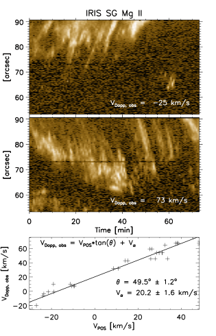
Figure 3: The top 2 panels show the time-distance diagram along part of the bottom-most slit position (tangent to the loop apex) at 2 wavelength positions. The slopes ($v_{\mathrm{POS}}$) of several paths of clumps are measured for each wavelength position ($v_{\mathrm{Dopp,obs}}$) and plotted in the bottom panel. Positive/negative slopes correspond, respectively, to negative/positive $V_{\mathrm{POS}}$.

Due to its position and orientation the IRIS slit captures a significant fraction of the loop near its apex (see Fig. 1). Hence, the slit captures the spectra of several flows directed along the loop. These flows produce positive / negative slopes for upward / downward flows, respectively, in the time-distance diagram along the slit (see Fig. 3). For each wavelength position (corresponding to a Doppler velocity $v_{\mathrm{Dopp,obs}}$, assuming the wavelength value from CHIANTI for the zero velocity, Dere et al., 2009) we select the most distinct paths and measure the slopes, which corresponds to the POS velocity along the slit $v_{\mathrm{POS}}$. These measurements are shown in the scatter plot of the bottom panel. The quantities follow the relation $v_{\mathrm{Dopp,obs}}=v_{\mathrm{POS}}tan(\theta)+v_{\mathrm{\alpha}}$, where $v_{\mathrm{\alpha}}$ corresponds to the zero Doppler velocity in the reference frame of the loop, and $\theta$ corresponds to the angle of the flow path (at the loop apex) with the POS plane. We find $\theta=49.5^{\circ}\pm 1.2^{\circ}$ and $v_{\mathrm{\alpha}}=20.2\pm 1.6$ km s^-1. This implies that the total velocity of a flow with POS velocity of 50 km s^-1 is close to 77 km s^-1, and that the transverse amplitude of the wave is $\approx 40~{}$km s^-1.

4 MHD Model

In order to interpret our observations, we set up a 2D MHD model of counter-streaming plasma clumps.

We consider a 2D spatial domain that extends for $12~{}$Mm in the $x-$direction (field aligned) and $6~{}$Mm in the $y-$direction. The magnetic field, $B_{0}$, is uniform and directed along the $x-$direction. Two trapezoidal clumps are placed at a distance of $4~{}$Mm and are $1~{}$Mm wide and $3~{}$Mm long in a background corona where the density is $n_{0}=1.2\times 10^{9}$ $cm^{-3}$ and the temperature is $T_{0}=1~{}$MK. The clumps are $n_{\mathrm{c}}$ times denser than the background plasma and colder in order to maintain pressure equilibrium. The plasma within the clumps has an initial velocity of $V_{\mathrm{B}}=\pm 70~{}$km s^-1. The shape of the clumps is such that the two facing sides are inclined in the same direction with an angle $\phi=50^{\circ}$. We numerically solve the set of ideal MHD equations using the MPI-AMRVAC software (Porth et al., 2014). We neglect non-ideal effects, as they would act on time scales longer than the observed evolution.

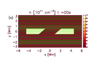
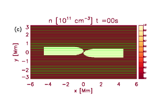
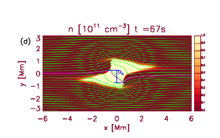
Figure 4: Maps of number density with overlaid magnetic field lines for the initial conditions of the simulations with trapezoidal or circular front clumps ((a) and (c)) and the times when the kink is maximum ((b) and (d)), for the strong collision scenario when $\beta=0.098$. The blue lines mark the amplitude $a_{k}$ of the kink. See also the accompanying animation.

The observations suggest lower and upper limits for the density contrast of the clumps. Therefore, we model a strong collision scenario where we have $n_{\mathrm{c}}=100$ and a weak collision scenario where we have $n_{\mathrm{c}}=25$. For each scenario we first run 4 simulations with different values of plasma $\beta$ ($0.02,0.05,0.2,0.5$) that defines a posteriori the field strength $B_{0}$. Fig. 4a illustrates the density and magnetic field lines in the initial condition for all simulations.

The clumps move towards one another and leads to the compression of plasma between the clumps, which is adiabatically heated up to $\sim 3$ MK and cools down to $750000$ $K$ in $\sim 10$ s due to mixing with the cold clump plasma. The pressure equilibrium no longer holds and the plasma expands in the $y-$direction leading to the distortion of the magnetic field. Because of the inclination of the facing sides of the clumps, the magnetic field is distorted at two different locations with an offset along the $x-$direction. This geometry leads to the kink of the magnetic field, as shown in Fig. 4b. The magnetic field lines threading the clumps appear all similarly distorted. After the initial kink of the magnetic field, the kink propagates along the clumps at the kink speed, which increases once the wave leaves the clumps. We measure the kink amplitude as the difference between the maximum and minimum $y-$coordinates of the magnetic field line crossing the origin at $t=0$ (blue lines marking in Fig. 4b).

As the kink is generated by the imbalanced thermal pressure due to the compression between the clumps, the amplitude of the kink depends on the background plasma $\beta$. For the strong and weak collision scenarios, we derive the kink amplitude as a function of $\beta$ and then, with a linear interpolation, we derive the best $\beta$ value to match the observed kink amplitude. We find that the kink amplitude increases until a maximum is reached and then reduces (Fig. 5a). As expected, the strong collision scenario leads to larger kink amplitudes and the higher the plasma $\beta$, the more the magnetic field is distorted. It is also evident that the wave period is longer for the larger plasma $\beta$ that implies the decrease in the Alfvén speed.

Fig. 5b shows the maximum kink amplitude for the two scenarios as a function of $\beta$. By means of this parameter space investigation, we derive that in the strong and weak collision scenarios the observed kink amplitude is matched when $\beta=0.09$ and when $\beta=0.36$, respectively. Therefore, by applying this simple model to the observed event we can constrain the value of the loop plasma $\beta$. While the initial distortion of the magnetic field is similar to a kink mode, once this travels away from the clumps, the amplitude of the remaining perturbation decreases and becomes more similar to a sausage mode (symmetric oscillation around $y=0$ axis). In particular for the strong collision scenario, this occurs between $\beta=0.05$ and $\beta=0.2$. For lower $\beta$, the collision is not strong enough to produce any significant long lasting oscillation and for higher $\beta$, the post collision magnetic field becomes so entangled that it no longer behaves as a wave guide. In the weak collision scenario we do not notice a visible persistence of sausage modes after the collision. Similarly, as long as the clumps’ collision is ongoing, the continued compression keeps the magnetic field kinked, but the magnetic field distortion location drifts towards the external part of the clumps. Only after the collision process is over, can the kink mode properly oscillate. Therefore, the wavelength of the initial kink oscillation depends on the length and speed of the clumps, as well as the plasma $\beta$.

To investigate the dependence on the shape of the clumps, we perform two more simulations (with the best $\beta$ values for both scenarios) where the two clumps are symmetric and have elliptic facing surfaces (Fig. 4c). Here, the central axes of the clumps are offset, overlapping for 75% of their width. In this configuration, the asymmetry that induces the kink is given by this offset. The kink amplitude (Fig. 4d) is found to be only $\sim 10\%$ smaller than in the simulation with trapezoidal clumps. Hence, although the presence of an asymmetry is crucial to produce a kink-like perturbation, the exact nature of this asymmetry (shape of interface or offset) appears unimportant in the current framework. We intend to pursue a more complete parameter space investigation to identify more exactly the role and nature of this asymmetry. Future 3D simulations will address more properties of this mechanism for the generation of kink and sausage waves, including the generation of torsional waves.

Figure 5: (a) Graph of the kink amplitude as a function of time for simulations with trapezoidal clumps. Solid and dashed lines correspond, respectively, to the strong and weak case scenario. (b) Maximum kink amplitude in each simulation as function of $Log_{\mathrm{10}}\left(\beta\right)$. Different colours mark the $\beta$ value: light blue, green, red, and blue for $\beta=0.02,0.05,0.2,0.5$, respectively. Magenta for the $\beta$ values that match best the observed kink amplitude in both scenarios.

5 Discussion and Conclusions

We have analysed coordinated observations with Hinode and IRIS of flows along a loop-like structure connecting a prominence with the solar surface. A collision between a downflow and an upflow is observed at estimated total speeds of $80~{}$km s^-1 and $60~{}$km s^-1, respectively (including Doppler and POS speeds). The densities of the flows are estimated to be around $6\times 10^{10}-3\times 10^{11}~{}$cm^-3. The flows are seen in SJI 2796 and 1400, indicating temperatures of $10^{4}-10^{5}$ K. At high resolution with SOT in the Ca II H line the flows appear clumpy, with widths of $0.3\arcsec-1.4\arcsec$. Coinciding with the time and location of collision, a bright and short-lived front is generated, indicating at least a 10 fold temperature increase. Also, at high resolution with SOT, these clumps are observed to oscillate transversely just after the collision, with an estimated total amplitude of $\approx 40~{}$km s^-1. We estimate a combined kinetic and enthalpy energy flux for these flows of $10^{7}-10^{8}$ erg cm^-2 s^-1.

Through 2D MHD numerical modelling, we have reproduced the collision between two counter-streaming flows with conditions similar to those observed. Since the clump densities are the least well-defined parameter, we allow a range of $25-100$ density contrast. Through a parameter space investigation, in order to reproduce the observed amplitude we find that the plasma $\beta$ must be confined between 0.09 and 0.36, which correspond, respectively, to magnetic field values of 6.5 G and 3.4 G.

The modelling indicates that the presence of asymmetry between the colliding clumps leads to the in-situ generation of trapped and leaky MHD waves, in particular transverse and sausage, which agrees with the initially out-of-phase (radial) oscillation of strands (characteristic of the sausage mode), followed by an in-phase transverse oscillation (characteristic of the kink mode). The observed increase in period is also well explained by the modelling: the wavelength of the transverse wave is set by the length of the clumps, which increases from the time of maximum compression. Transverse MHD waves may therefore be generated in-situ in the corona through flow collision. For cool and dense prominence conditions such waves could have significant amplitudes.

The temperature at the collision can increase to coronal values, explaining the sudden intensity increase in all 3 channels. No localised signature was found in the SDO/AIA channels (excluding AIA 304), possibly due to the increased LOS integration or long ionisation times. Nonetheless, similar signatures of counter-streaming flows and transverse MHD waves are observed at other times in this structure. The cumulative effect of such flow collisions (possibly explaining the observed background oscillation) and in-situ generated transverse MHD waves (particularly the compressive waves) may contribute to the energy balance, which may explain the EUV emission of the entire structure.

References

- Alexander et al. (2013) Alexander, C. E., Walsh, R. W., Régnier, S., et al. 2013, ApJ, 775, L32
- Antiochos et al. (1999) Antiochos, S. K., MacNeice, P. J., Spicer, D. S., & Klimchuk, J. A. 1999, ApJ, 512, 985
- Antolin & Rouppe van der Voort (2012) Antolin, P., & Rouppe van der Voort, L. 2012, ApJ, 745, 152
- Antolin et al. (2010) Antolin, P., Shibata, K., & Vissers, G. 2010, ApJ, 716, 154
- Antolin et al. (2015) Antolin, P., Vissers, G., Pereira, T. M. D., Rouppe van der Voort, L., & Scullion, E. 2015, ApJ, 806, 81
- Arregui (2015) Arregui, I. 2015, Philosophical Transactions of the Royal Society of London Series A, 373, 20140261
- Arregui et al. (2012) Arregui, I., Oliver, R., & Ballester, J. L. 2012, Living Reviews in Solar Physics, 9, 2
- De Moortel & Nakariakov (2012) De Moortel, I., & Nakariakov, V. M. 2012, Royal Society of London Philosophical Transactions Series A, 370, 3193
- De Pontieu et al. (2014) De Pontieu, B., Title, A. M., Lemen, J. R., et al. 2014, Sol. Phys., 289, 2733
- Dere et al. (2009) Dere, K. P., Landi, E., Young, P. R., et al. 2009, A&A, 498, 915
- Hillier et al. (2013) Hillier, A., Morton, R. J., & Erdélyi, R. 2013, ApJ, 779, L16
- Karpen et al. (2001) Karpen, J. T., Antiochos, S. K., Hohensee, M., Klimchuk, J. A., & MacNeice, P. J. 2001, ApJ, 553, L85
- Keppens & Xia (2014) Keppens, R., & Xia, C. 2014, ApJ, 789, 22
- Kleint et al. (2014) Kleint, L., Antolin, P., Tian, H., et al. 2014, ApJ, 789, L42
- Kosugi et al. (2007) Kosugi, T., Matsuzaki, K., Sakao, T., et al. 2007, Sol. Phys., 243, 3
- Landi & Reale (2013) Landi, E., & Reale, F. 2013, ApJ, 772, 71
- Lemen et al. (2011) Lemen, J. R., Title, A. M., Akin, D. J., et al. 2011, Sol. Phys., 172
- Lin (2011) Lin, Y. 2011, Space Sci. Rev., 158, 237
- Lin et al. (2005) Lin, Y., Engvold, O., Rouppe van der Voort, L., Wiik, J. E., & Berger, T. E. 2005, Sol. Phys., 226, 239
- Ning et al. (2009) Ning, Z., Cao, W., Okamoto, T. J., Ichimoto, K., & Qu, Z. Q. 2009, A&A, 499, 595
- Ofman & Wang (2008) Ofman, L., & Wang, T. J. 2008, A&A, 482, L9
- Okamoto et al. (2015) Okamoto, T. J., Antolin, P., De Pontieu, B., et al. 2015, ApJ, 809, 71
- Okamoto et al. (2007) Okamoto, T. J., Tsuneta, S., Berger, T. E., et al. 2007, Science, 318, 1577
- Pesnell et al. (2012) Pesnell, W. D., Thompson, B. J., & Chamberlin, P. C. 2012, Sol. Phys., 275, 3
- Porth et al. (2014) Porth, O., Xia, C., Hendrix, T., Moschou, S. P., & Keppens, R. 2014, ApJS, 214, 4
- Schmieder et al. (2013) Schmieder, B., Kucera, T. A., Knizhnik, K., et al. 2013, ApJ, 777, 108
- Suematsu et al. (2008) Suematsu, Y., Tsuneta, S., Ichimoto, K., et al. 2008, Sol. Phys., 249, 197
- Tsuneta et al. (2008) Tsuneta, S., Ichimoto, K., Katsukawa, Y., et al. 2008, Sol. Phys., 249, 167
- Vial & Engvold (2015) Vial, J.-C., & Engvold, O., eds. 2015, Astrophysics and Space Science Library, Vol. 415, Solar Prominences (Springer International Publishing Switzerland)
- Xia et al. (2017) Xia, C., Keppens, R., & Fang, X. 2017, A&A, 603, A42