ALMA reveals molecular cloud N 55 in the Large Magellanic Cloud as a site of massive star formation

Abstract

We present the molecular cloud properties of N 55 in the Large Magellanic Cloud using ¹²CO(1-0) and ¹³CO(1-0) observations obtained with Atacama Large Millimeter Array. We have done a detailed study of molecular gas properties, to understand how the cloud properties of N 55 differ from Galactic clouds. Most CO emission appears clumpy in N 55, and molecular cores that have YSOs show larger linewidths and masses. The massive clumps are associated with high and intermediate mass YSOs. The clump masses are determined by local thermodynamic equilibrium and virial analysis of the ¹²CO and ¹³CO emissions. These mass estimates lead to the conclusion that, (a) the clumps are in self-gravitational virial equilibrium, and (b) the ¹²CO(1-0)-to-H₂ conversion factor, X_CO, is 6.5$\times$10²⁰ cm^-2 (K km s^-1)^-1. This CO-to-H₂ conversion factor for N55 clumps is measured at a spatial scale of $\sim$0.67 pc, which is about two times higher than the X_CO value of Orion cloud at a similar spatial scale. The core mass function of N 55 clearly show a turnover below 200 M_⊙, separating the low-mass end from the high-mass end. The low-mass end of the ¹²CO mass spectrum is fitted with a power law of index 0.5$\pm$0.1, while for ¹³CO it is fitted with a power law index 0.6$\pm$0.2. In the high-mass end, the core mass spectrum is fitted with a power index of 2.0$\pm$0.3 for ¹²CO, and with 2.5$\pm$0.4 for ¹³CO. This power-law behavior of the core mass function in N 55 is consistent with many Galactic clouds.

1 Introduction

Most stars form as clusters in Giant Molecular Clouds (GMCs) which encompass cold molecular gas and dust with masses $\sim$10^4-5M_⊙. Therefore, understanding the evolution of dust and gas in GMCs is important to understand the formation of stars in galaxies. The GMCs are composed of sub-parsec-sized clumps, the size of which is determined by the forces of gravity and magneto-turbulent pressure. Stars form inside these clumps, hence a detailed understanding of the star formation process requires a sub-parsec scale resolution view of GMCs and accurate measurements of the physical parameters of these clumps. Star formation requires high-density clumps where most of the interstellar hydrogen should be in the form of molecular, H₂. Since H₂, in the form of cold molecular gas, is almost totally undetectable with observations, emission from the tracer CO and its isotopes is widely used in galaxies to estimate the molecular core properties and distribution of GMCs. There have been large-scale molecular surveys undertaken in ¹²CO(1-0) and ¹³CO(1-0) emission of the Galactic clouds to unveil distribution, structure and physical properties of molecular clumps (Dame et al., 1987; Combes, 1991; Mizuno et al., 1995; Onishi et al., 1996). Infrared observations of these molecular clouds have revealed young stellar objects (YSOs) embedded in dense molecular cores, that strongly suggest on-going star formation. ¹³CO emission often can be optically thin and traces dense molecular gas, therefore it can be used to study the relationship between YSOs and their parent molecular cloud (Bally, 1989; Fukui & Mizuno, 1991). Similar observations at high spatial resolution in Galactic clouds have been extended to much denser molecular tracers, such as NH₃, CS, HCN, and HCO⁺ (Myers, 1987; Zhou et al., 1989; Myers, 1983; Stutzki & Guesten, 1990). These authors found that small dense cores, with size $\sim$ 0.1 pc and density n$\sim$10⁴ cm^-3 are the sites for massive star formation, and physical conditions of cores are closely related to the properties of embedded YSOs.

There is an extensive literature available on determining the physical parameters of clumps in Galactic molecular clouds and their relationships to star formation. Many of these studies focus on GMC scaling relations between observable quantities such as size, velocity dispersion, mass surface density, etc. Larson (1981) reported three empirical scaling relations for clump basic parameters in Milky Way GMCs. Those are: 1) a power law relation between velocity dispersion and size of emitting medium, $\sigma_{v}\propto R^{0.38}$; 2) molecular clouds are virialized, $2\sigma_{v}R^{2}/GM\sim 1$; 3) mean density of cloud is inversely related to size, $n\sim R^{-1.1}$. The Larson scaling relationships have been later tested with observations in various molecular tracers including rotational transitions of CO, its isotopes and denser molecular tracers such as NH₃, CS, HCN, and HCO⁺ (Dame et al., 1986; Scoville et al., 1986; Solomon et al., 1987; Zhou et al., 1989; Hobson, 1992; Myers, 1983; Tatematsu et al., 1998; Heyer et al., 2001, 2009; Ikeda et al., 2009). Many of these studies reveal power law relationships between the velocity dispersion and size indicating self-gravitating clouds in virial equilibrium with a power law index ranging from 0.25 to 0.75. In contrast, Oka et al. (2001) reported large velocity dispersion in the Galactic center clouds with ¹²CO(1-0) observations, showing a deviation from a power law relation between velocity dispersion and radius. Their studies indicate the requirement of external pressure for cloud equilibrium confinement. Spatially resolved studies of molecular gas properties in the Large Magellanic Cloud (LMC), as well as certain dwarf galaxies and local group spiral galaxies, show similar GMC characteristics as those found in the Milky Way (Bolatto et al., 2008; Fukui et al., 2008; Hughes et al., 2010; Wong et al., 2011). The GMCs in these galaxies show similar size, linewidths and masses as in Galactic clouds. However, observation of CO lines in metal-poor dwarf galaxies indicates extremely weak CO luminosity compared to their star formation rates. The CO luminosity to star formation rate ratio tends to decrease with decreasing metallicity, although the dwarf galaxies may still follow the Kennicutt-Schmidt relationship depending on how the H₂ mass is accounted for (Ohta et al., 1993; Taylor et al., 1998; Schruba et al., 2012; Cormier et al., 2014). Observations suggest that in metal-poor galaxies, the clump properties and hence star formation process may differ from those in metal-rich environments due to hard radiation field from newly formed stars. Due to reduced dust shielding and molecular gas abundances, radiation can penetrate more deeply into the molecular cloud and may produce a clumpier cloud (Madden et al., 2006; Rémy-Ruyer et al., 2013).

Spatially resolved CO observations in large-scale surveys have been carried out in the nearest low-metallicity galaxy, the LMC, with an aim to investigate whether the GMC characteristics and star formation conditions follow universal patterns. The LMC is an excellent site to explore the GMC characteristics in a sub-solar metallicity (0.5 Z_⊙) due to its proximity (50 kpc) and favorable viewing angle (Pietrzyński et al., 2013; van der Marel & Cioni, 2001). The clumpy structures have been revealed in CO observations of the LMC molecular clouds. For example, the observations of ¹²CO and ¹³CO in J=1-0, 2-1, 3-2 and 4-3 transitions have revealed the dense and hot molecular clumps, along with detailed physical properties of the molecular gas at a spatial resolution of $\sim$5 pc in H ii regions (Minamidani et al., 2008, 2011). These observations were done at an angular resolution $\sim$ 23^′′, which cannot resolve the clump sub-structures at the LMC distance, 50 kpc (Pietrzyński et al., 2013). The large-scale CO surveys in the LMC molecular clouds include: 12^′ resolution map of ¹²CO(1-0) with 1.2 m Columbia Millimeter-Wave Telescope; 2.6^′ resolution map of ¹²CO(1-0) with the NANTEN 4 m telescope; 45^′′ resolution ¹²CO(1-0) targeted mapping of known CO clouds from NANTEN survey with the Mopra telescope (MAGMA Wong et al. (2011)); 1^′ resolution individual cloud mapping in ¹²CO(1-0) with the Swedish-ESO Submillimetre Telescope (SEST). Fukui et al. (2008) report the CO-to-H₂ conversion factor to be 7$\times$10²⁰ cm^-2(K km s^-1)^-1 for the molecular clouds in the LMC from the NANTEN survey at angular resolution 2.6^′. The size-linewidth relation is found to be consistent with the power law relation proposed by Larson (1981) with power law index of 0.5. Wong et al. (2011) report a much steeper power law relation for size and velocity dispersion. They suggest that this power law relation may break down when the structures are decomposed into smaller structures.

In addition, there has been high spatial resolution (sub-parsec) mapping of ¹²CO(2-1) and ¹³CO(2-1) observations with the Atacama Large Millimeter Array (ALMA) in the active star-forming regions, 30 Doradus and N 159 west, of the LMC (Indebetouw et al., 2013; Fukui et al., 2015). Indebetouw et al. (2013) report relatively high velocity dispersions for 30 Doradus clouds and a power law relation inconsistent with those found for Galactic clouds. They suggest the large velocity dispersions for 30 Doradus clouds must be due to pressure confinement where an external force is necessary to hold clumps in equilibrium. Furthermore, the dust mass is found to be a factor of 2 lower than the average value of the LMC, indicating a reduced dust-to-gas mass ratio in 30 Doradus. Fukui et al. (2015) identified protostellar outflows toward two young high-mass stars along with an indication of colliding filaments in N 159 west using ¹³CO(2-1) mapping at sub-parsec scale resolution. These observations necessitate a further study of GMC properties in an LMC molecular cloud, where the star formation activity should be comparable to many other Milky Way clouds abiding Larson’s scaling relations.

This paper examines the molecular clump properties such as size, velocity dispersion, mass, and their association to star formation in N 55 region of the LMC. This region is less extreme than the well studied 30 Doradus or N 159 environments. We choose this cloud based on our infrared spectroscopic and photometric observations with Spitzer and Hershel space telescopes as part of Surveying the Agents of Galaxy Evolution (SAGE) and the Herschel Inventory of the Agents of Galaxy Evolution (HERITAGE) of the LMC (Meixner et al., 2006, 2010). With infrared spectrograph on Spitzer (as part of SAGE), we have detected the H₂ rotational transitions at 28.2 and 17.1${\,\rm\mu m}$ (Naslim et al., 2015) in N55. The clumpy and filamentary structures of H₂ emission in N 55 spatially resemble the distribution of polycyclic aromatic hydrocarbon (PAH) emission traced by Spitzer InfraRed Array Camera (IRAC) 8.0${\,\rm\mu m}$ as well as the dust emission traced by Herschel Photodetector Array Camera and Spectrometer (PACS) 100${\,\rm\mu m}$. A detailed analysis of the infrared observations of this region will be presented in a future paper. In this paper, we aim to determine how (dis-)similar the N 55 clumps are from Milky Way clumps and 30 Doradus. We study the molecular clump scaling relations of N 55 and investigate whether the power law relations for Milky Way clouds hold in a sub-solar metallicity environment.

2 N 55 molecular cloud

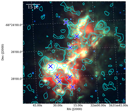
Figure 1: The structure of N 55 is shown in a composition of three color map: in blue, Spitzer IRAC 5.8${\,\rm\mu m}$ which traces infrared bright sources, in green Spitzer IRAC 8.0${\,\rm\mu m}$ which traces the PAH emission and in red MIPS 24${\,\rm\mu m}$ tracing hot dust heated by hard radiation from massive stars. The hot stars from Olsen et al. (2001) are labelled in crosses. For comparison, ¹²CO(3-2) emission observed with ASTE is shown in contours, tracing warm molecular gas.

N 55 is located inside LMC 4, the largest Supergiant Shell (SGS) in the LMC (Yamaguchi et al., 2001). The LMC 4 has a diameter of about 1.5 kpc. A study of the H${\alpha}$ map by Olsen et al. (2001) shows that the H ii region of N 55 may be excited by a young cluster, LH 72, containing at least 8 O and B type stars. Olsen et al. (2001) also reported the LMC 4 was not formed as a unit, but by overlapping shells, and N 55 seems to be associated with one of the overlapping shells SGS 14, which may have triggered the formation of LH 72. Therefore N 55 seems to be located in an environment of multiple supernova explosions, the most recent one being SGS 14. Complex filamentary structures are especially prominent toward N 55 in Spitzer SAGE images (Figure 1), which show the distribution of hot gas and photo-dissociated PAHs in the interstellar medium. These filamentary structures may be due to instabilities enhanced by shocks. Shocks of supernova explosions are reported to be a cause of the enhanced filamentary structures and dense clumps in molecular clouds (Ntormousi et al., 2011). The clumpy nature of the molecular gas in N 55 is revealed by ¹²CO(3-2) emission observed with Atacama Submillimeter Telescope Experiment (ASTE) (Figure 1). The interior of LMC 4 is otherwise almost empty of ionized and atomic gas, while N 55 stands out as a bright H ii region in H${\alpha}$ map (Olsen et al., 2001). The formation of LMC 4 and the survival of N 55 have been debated for a decade. Suggestions include supernova explosions, gamma ray bursts, stellar winds from massive stars in LH 72 or stochastic propagation of star formation which have cleared out the gas from the interior (Book et al., 2009). Book et al. (2009) suggest that star formation was likely triggered by the compression of a pre-existing cloud in the expanding shell, LMC 4, as evidenced by the distribution and kinematics of the gas in the expanding LMC 4 (Israel et al., 2003). Based on the Spitzer colors of point sources, Gruendl & Chu (2009) and Seale et al. (2014) identified 16 YSOs in N 55 indicating on-going star formation.

3 Observations

N 55 was observed with ALMA in cycle 1 & 2 ( 2013.1.00214.S and 2012.1.00335.S), using band 3 receivers in spectral windows centered at 115.27, 110.20 and 109.67 GHz with 70.557 kHz (0.2 km s^-1) spectral resolution. The area of coverage was 4${}^{\prime}\times$6^′ at the center position: right ascension $\sim 05^{\rm h}32^{\rm m}15^{\rm s}.49$ and declination $\sim-66^{\rm o}26^{\prime}14^{\prime\prime}.00$. In each spectral window, the correlator was set to have a bandwidth of 117.18 MHz. Uranus and Ganymede were used as flux calibrators. The data were processed in the Common Astronomy Software Application (CASA) package and visibilities imaged. The synthesized beam for ¹²CO(1-0) is approximately 3.5${}^{\prime\prime}\times$2.3^′′ which corresponds to 0.84$\times$0.55 pc². The achieved rms per channel over 0.2 km s^-1 is about $\sim$70 mJy beam^-1 (0.8 K). For ¹³CO(1-0) the synthesized beam is about 3.1${}^{\prime\prime}\times$2.5^′′ which corresponds to 0.74$\times$0.60 pc², and the achieved sensitivity per channel over 0.2 km s^-1 is 20 mJy beam^-1 (0.30 K). Note that, our ¹³CO(1-0) data are three times more sensitive than the ¹²CO(1-0) data, due to the longer integration time and four repeated observations of the ¹³CO. The details of observations are given in Table 1. The typical system noise temperatures of the ¹²CO and the ¹³CO are $\sim$170 K and $\sim$90 K. We use a moment masked cube (Dame, 2011) to suppress the noise effect in our analysis. The moment masked cube has zero values at the emission free pixels, which is useful to avoid a large error arising from the random noise. The emission-free pixels are determined by identifying significant emission from the smoothed data whose noise level is much lower than the original data. The caveat of this method is that it eliminates small clouds with low peak intensity because we smooth the data both for the velocity and spatial directions (Dame, 2011). In order to determine the fraction of missing flux caused by interferometric observation with ALMA 12 m array, we compare our data with the single dish Mopra observation of ¹²CO(1-0). About 30$\%$ of the ALMA flux is missing when smoothed to 45” and compared to the Mopra observations.

Table 1: Observations

12CO(1-0)			13CO(1-0)
Execution Block	Date	Integration time	Execution Block	Date	Integration time
		(minutes)			(minutes)
uid://A002/X98ed3f/X1cf5	2015-01-06	70	uid://A002/X77da97/X177	2013-12-31	55
			uid://A002/X77da97/X836	2014-01-01	51
			uid://A002/X98ed3f/X21cf	2015-01-06	65
			uid://A002/X9a24bb/X1460	2015-01-22	57

4 Molecular gas distribution in N 55

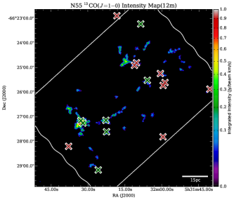
Figure 2: ¹²CO(1-0) (left) and ¹³CO(1-0) (right) integrated intensity maps of N 55. The YSOs identified with Spitzer (green-white crosses) and Herschel (red-white crosses) are labelled (Gruendl & Chu, 2009; Seale et al., 2014).

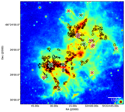
Figure 3: ¹²CO(1-0) emission in contours on IRAC 8.0${\,\rm\mu m}$ map. The contour levels are 0.09, 1.5, 3.0, 4.5, 6.0, and 9.0 Jy beam^-1 km s^-1. The YSOs identified with Spitzer (green-white crosses) and Herschel (red-white crosses) are labelled (Gruendl & Chu, 2009; Seale et al., 2014)

Our ¹²CO(1-0) and ¹³CO(1-0) observations with ALMA show the clumpy nature of molecular gas in N 55 at sub-parsec scale (Figure 2). It is clearly seen by eye that compact molecular clumps are distributed along the filamentary structure of PAH emission traced by IRAC 8.0${\,\rm\mu m}$ (Figure 3). The ¹²CO(1-0) integrated intensity map appears to be relatively extended, compared to that of its isotopologue ¹³CO(1-0) which is clumpier and most of the clumps are clearly delineated by the Spitzer-identified YSO candidates (Table 2). These YSO positions are shown in Figure 2 along with ¹²CO(1-0) and ¹³CO(1-0) integrated intensity maps. Many clouds show numerous sub-clumps and these sub-clumps (molecular cores) are associated with YSOs. The filamentary structures traced by ¹²CO(1-0) follows that of the PAHs traced by IRAC 8.0${\,\rm\mu m}$ map (Figure 3). These observations may indicate that the CO is mostly excited in the same regions where the dust is photoelectrically heated by ultraviolet radiation. Since the structure is very complex, we identify the clumps and determine their properties using a dendrogram method.

5 Molecular mass determination

Figure 4: Excitation temperature map of N 55 which is derived from ¹²CO(1-0) emission using equation 2.

We determine the molecular gas mass using virial and local thermodynamic equilibrium (LTE) assumptions. In order to determine the LTE mass ($M_{\rm LTE}$) from ¹³CO(1-0) emission, we need to calculate column density and assume that the excitation temperature for ¹³CO(1-0) is the same as the ¹²CO(1-0) emission. To derive the ¹³CO(1-0) column density we follow the method given by Dickman (1978), Pineda et al. (2008), Pineda et al. (2010) and Nishimura et al. (2015). Assuming that the emission is optically thin and in LTE, we derive the column density using the following formula (Pineda et al., 2008).

$$N(^{13}{\rm CO})=3.0\times 10^{14}\left(\frac{\tau(^{13}{\rm CO})}{1-e^{-\tau}}\right)\left(\frac{W({\rm CO})}{1-e^{-5.3/T_{{\rm ex}}}}\right)$$ (1)

In equation 1, $W$(CO) is the integrated intensity ($\sum{T_{{\rm mb}}}dv$) of ¹³CO(1-0) in K km s^-1. To derive column density of ¹³CO(1-0), we require the excitation temperature $T_{\rm ex}$ and optical depth $\tau$. The excitation temperature $T_{\rm ex}$ at each position in 0.2 km s^-1 wide channel is determined from the peak temperature ($T_{{}^{12}\rm CO}$) of the optically thick ¹²CO line.

$$T_{{\rm ex}}=\frac{5.5\,{\rm K}}{{\rm ln}\{1+5.5\,{\rm K}/[T(^{12}{\rm CO})+0.82\,\rm{K}]\}}$$ (2)

Using the excitation temperature derived from the above equation we calculate ¹³CO optical depth for each position in 0.2 km s^-1 wide channel along the line of sight using the following equation:

$$\tau(^{13}{\rm CO})=-{\rm ln}\left[1-\frac{T_{{\rm max}}/5.3}{1/({\rm e}^{5.3/T_{{\rm ex}}}-1)-0.16)}\right]$$ (3)

Here $T_{\rm max}$ is the main beam brightness temperature at the peak of the ¹³CO emission.

The assumption of optically thin ¹³CO(1-0) emission and identical excitation temperatures for ¹³CO(1-0) and ¹²CO(1-0) in LTE, may cause several systematic errors in mass determination. In reality, the excitation condition for ¹²CO(1-0) and ¹³CO(1-0) is not the same throughout the cloud, as both these emission sample different volume densities. Moreover, the excitation of ¹³CO(1-0) is not fully thermalized in most of the cloud volume, however ¹²CO(1-0) can be thermalized even at densities lower than ¹²CO critical density ($n$H${}_{2}<$750 cm³). Heyer et al. (2009) have quantitatively checked these effects by comparing the column densities derived by the LTE method with models obtained for several sets of cloud conditions using a large velocity gradient (LVG) approximation. They found that the LTE method can either underestimate or overestimate the input column density. In our study the typical densities of the cloud is $n$H${}_{2}>1000$ cm^-3. Based on Figure 6 in Heyer et al. (2009) the ratio of LTE to LVG model masses is around unity, however there is a scatter about 40$\%$.

We derive the total molecular gas mass using ¹³CO(1-0) column density and the molecular abundance ratios [¹²CO/¹³CO] and [¹²CO/H₂]. We adopt abundance ratios of 50 for [¹²CO/¹³CO] and 1.6$\times$10^-5 for [¹²CO/H₂] which were derived for N 159 in the LMC (Mizuno et al., 2010). Hence, we obtain an H₂ column density of $N({\rm H_{2}})=\frac{50}{1.6\times 10^{-5}}N(^{13}\rm CO)$. Finally, the molecular gas mass is calculated from $N({\rm H_{2}}$) at the LMC distance, assuming that the mean molecular weight per H₂ is 2.7.

We applied the above formula to molecular clumps of ¹³CO(1-0) obtained with our clump decomposition method astrodendro (section 6) and derived the LTE mass $M_{{\rm LTE}}$ for each clump, where the excitation temperature of ¹³CO(1-0) is obtained from the $T_{\rm ex}$ map (Figure 4) derived from equation 2.

In addition to the LTE mass, we derive virial masses for ¹³CO(1-0) and ¹²CO(1-0) clumps. We assume that clouds are spherical with a truncated density profile, $\rho\sim$r^-1, and derive the virial mass from the radius (R) and velocity dispersion ($\sigma_{v}$) of the clump (Wong et al., 2011) as,

$$M_{\rm VIR}[M_{\odot}]=1040\sigma_{v}^{2}R$$ (4)

6 Clump decomposition using astrodendro

The structure of molecular clouds is highly hierarchical. Small scale dense molecular cores are invariably enclosed within the envelope of large scale lower density gas (Lada, 1992). These sub-parsec scale ($\sim$0.1 pc) dense cores are the sites for high mass star formation inside molecular clouds. Probing the properties such as mass, radius and velocity dispersion of these cores, allow us to understand the mass function as well as conditions for star formation because of their close relationship with newly formed stars (di Francesco et al., 2007). In order to determine the properties of molecular clouds in ¹³CO(1-0) and ¹²CO(1-0) emission, we use the python package astrodendro. The concept of dendrograms to characterize the structures of molecular gas as a ”structure tree” in a three-dimensional data cube was first introduced by Houlahan & Scalo (1992). A more systematic way of a clump-finding algorithm using a dendrogram method was later implemented by Rosolowsky et al. (2008), who showed how to graphically represent the hierarchical structure of nested isosurfaces in three-dimensional data cubes. A dendrogram is composed of leaves and branches where each entity in the dendrogram is represented as an isosurface (three-dimensional contour) in the data cube. The leaves are the brightest and smallest structures that represent three-dimensional contours with single local maxima. The local maxima represent the top level of the dendrogram which are the brightest structures (dense molecular cores) that we refer as leaves. Branches represent parent structures which connect two leaves and form larger structures that represent lower density media. Finally, all leaves and branches merge together to form trunks of the tree. In this paper molecular cores are the structures which are identified as dendrogram leaves. Most of the leaves are of sub-parsec scale size. The clumps are those identified as dendrogram trunks which are mostly of parsec scale size. A cluster of clumps and cores is referred to as a cloud. With the use of dendrogram, we can represent the complexity of molecular clouds effectively over a range of size scales starting from low-density gas in the bottom level.

Astrodendro identifies unique isosurfaces from each region of emission in a three-dimensional data cube and computes the properties based on the moment of volume weighted intensities of emission from every pixel (Rosolowsky et al., 2008). The data cube consists of two spatial dimensions (X and Y) and a velocity dimension (V). The rms sizes (Colombo et al., 2015) of a clump in two spatial dimensions ($\sigma_{\rm x}$ and $\sigma_{\rm y}$), i.e. along the major axis and minor axis are computed from the intensity-weighted second moments in two dimensions, dx and dy. The geometric mean of these second spatial moment along the major and minor axis of the clump is the final rms radius of a clump ($\sigma_{r}$). The rms radius in the second spatial moments obtained from astrodendro is converted into the radius of a spherical cloud $R=1.91\sigma_{r}$ (Solomon et al., 1987).

The velocity dispersion, $\sigma_{v}$, is the intensity-weighted second moment of the velocity axis. The sum of all emission within an isosurface is the flux of a clump (F=$\sum{T_{i}dxdydv}$), where $T_{i}$ is the brightness temperature. The luminosity of a clump is the integrated flux scaled by the square of the distance to the object in parsec.

$$L_{{\rm CO}}[{\rm K\,km\,s^{-1}\,pc^{2}}]=D^{2}\sum(T)dxdydv$$ (5)

To determine the uncertainties in the derived parameters, we use a bootstrapping technique similar to the method given in Rosolowsky et al. (2008). We use 100 iterations to sample the derived parameters. Tables 3 and 4 list ¹²CO and ¹³CO clump (${\it astrodendro}$ trunk) properties.

The size and linewidth determinations can be biased by the limited instrumental resolution and sensitivity. This can be particularly important when the extent of the intensity distribution is comparable to the instrumental profile, e.g., the structures have sizes similar to or less than the beam width. Rosolowsky & Leroy (2006) applied a correction for this bias by extrapolating the size, linewidth, and flux to a zero noise level and then deconvolving the instrumental resolution. To determine the deconvolved sizes, for instance, they subtracted the rms beam size from the extrapolated spatial moments along the major and minor axes of the clump, ($\sigma_{x}$, $\sigma_{y}$), in quadrature. They found that without deconvolution, the resolution effect can exaggerate the clump size by $\sim$40$\%$, and that applying their deconvolution method recovers the size to within 10$\%$ for S/N ratios greater than 5. The chief drawback to this approach is the required extrapolation to the zero intensity level, which is much less reliable for blended structures (such as clumps within a molecular cloud) than for isolated, discrete structures. For instance, Wong et al. (2008) showed that extrapolation increases the ¹³CO clump masses in the RCW 106 GMC by roughly an order of magnitude, violating the limit imposed by the total map flux. On the other hand, deconvolution without extrapolation would lead to an underestimation of the sizes of structures and lead to many of the smallest structures (what we refer to as cores) having unreliable size because their apparent sizes (above a noise threshold) are less than the beam size. Thus, instead of attempting to correct for instrumental resolution, we indicate the regions (as shaded blue) where the resolution significantly affects the values in the histogram and correlation plots (Figures 5, 6 and 10). The channel width divided by $\sqrt{8\,{\rm ln}\,2}$ is taken as resolution in $\sigma_{v}$, and the beam width multiplied by 1.91 and divided by $\sqrt{8\,{\rm ln}\,2}$ is taken as resolution in radius Wong et al. (2017). In our analysis the sizes of all identified dendrogram trunks are above the resolution limit ($\sim 0.55$ pc), hence these structures are large enough to resolve the clumps. About 30$\%$ of the dendrogram leaves are having a size below the resolution limit which are the smallest structures in the dendrogram. We do not consider those as reliable structures.

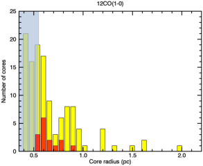
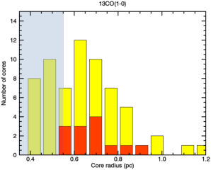
Figure 5: Histograms of ¹²CO (left) and ¹³CO (right) core radii with (red) and without (yellow) YSOs. The shaded blue indicates the region where the observational resolution affects the sizes.

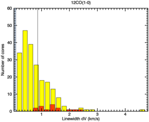
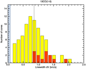
Figure 6: Histograms of ¹²CO (left) and ¹³CO (right) core linewidths with (red) and without (yellow) YSOs. Thermal and turbulent molecular cores are separated by the vertical lines at 0.861 km s^-1 (¹²CO) and 0.863 km s^-1 (¹³CO). The shaded blue indicates the region where the observational resolution affects the linewidths.

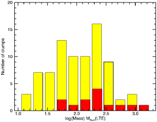
Figure 7: Histograms of ¹³CO core LTE masses with (red) and without (yellow) YSOs.

7 Results

7.1 Molecular clump properties and association with YSOs

Our dendrogram analysis on ¹³CO(1-0) and ¹²CO(1-0) emission provides the cloud properties such as size, velocity dispersion, and mass of N 55. We use these properties to understand the close relation of star formation with molecular cores. We derive the apparent velocity width $\Delta V$, FWHM, of each clump by multiplying the velocity dispersion $\sigma_{v}$ with $2\sqrt{2{\rm ln}2}$, assuming a Gaussian distribution.

We compare the sizes and velocity widths of molecular clumps in N 55 with YSOs and those without YSOs. For this purpose, we choose the molecular cores in ¹³CO(1-0) and ¹²CO(1-0) emission that are identified as leaves (Tables 5 and 6) with astrodendro where the stars are assumed to be formed. The size distribution of ¹³CO(1-0) and ¹²CO(1-0) cores are given as histograms in Figure 5. Radii of ¹³CO(1-0) dense cores with YSOs range from 0.55 to 0.9 pc and those with larger 0.95–1.2 pc do not show YSOs. In Figure 5, the shaded blue indicates the region where the observation resolution affects the sizes. About 30$\%$ of CO cores have sizes less than the instrumental resolution, those we do not consider as relevant structures in our analysis. The positions of all identified YSOs and associated molecular clumps are given in Table 2.

The velocity width distributions for ¹²CO(1-0) and ¹³CO(1-0) emission are shown in Figure 6. Those with YSOs are shown (in red) for comparison. We note that YSOs are embedded within ¹³CO(1-0) dense cores with larger velocity widths (0.9–2.0 km s^-1). The distribution of ¹²CO(1-0) velocity widths shows a peak at 0.4 km s^-1 and the velocity width tail extends up to 4.6 km s^-1. The ¹²CO(1-0) velocity widths for star forming cores range from 0.8–2.5 km s^-1. The ¹³CO(1-0) velocity widths peak at 0.8 km s^-1 and show a velocity width tail extending up to 2.1 km s^-1. The large velocity width in general suggests the effect of internal turbulence in molecular cores. If the observed velocity width is higher than the thermal velocity width, the molecular cores are expected to be dominated by non-thermal motions.

According to Myers et al. (1991) and Ikeda et al. (2007), the massive star-forming cores with turbulent and thermal motion can be differentiated on the basis of their critical velocity width, $dv_{cr}$, at which thermal and nonthermal velocity components are equal. The cores are considered to be thermal or nonthermal if the nonthermal velocity component is significantly less than or greater than the thermal velocity. Therefore, the cores with observed velocity width greater than the $dv_{cr}$ is considered as turbulent. In figure 6 we indicate the critical velocity widths calculated from equation 8 of Ikeda et al. (2007) for ¹³CO(1-0) and ¹²CO(1-0) with the vertical lines at 0.861 and 0.863 km s^-1 respectively. We note that all star-forming ¹³CO(1-0) and ¹²CO(1-0) cores, have linewidths $\geq dv_{cr}$, indicating some effect of turbulence. In Figure 7, we compare the distribution of LTE masses of molecular cores with (red) and without (yellow) YSOs. We find that 50$\%$ of massive cores ($\geq$500M_⊙) are associated with YSOs.

Figure 8 shows the relationship between LTE and virial masses for clumps with YSOs and those without YSOs. The relationship is fitted with a power law of $M_{{\rm VIR}}$=1.75$M_{{\rm LTE}}^{0.68\pm 0.12}$ with a correlation coefficient 0.8 which indicates a tight correlation. The ratio of LTE mass to virial mass shows an average value of 1.12, including all star-forming and non-star-forming clumps. The star-forming clumps cluster around the power law line $M_{{\rm VIR}}$=1.75$M_{{\rm LTE}}^{0.68\pm 0.12}$. Three massive clumps with YSOs have LTE masses three times larger than their virial masses, and all other star-forming clumps have LTE masses consistent with virial masses. These results indicate that most of the star-forming and non-star-forming cores are gravitationally bound.

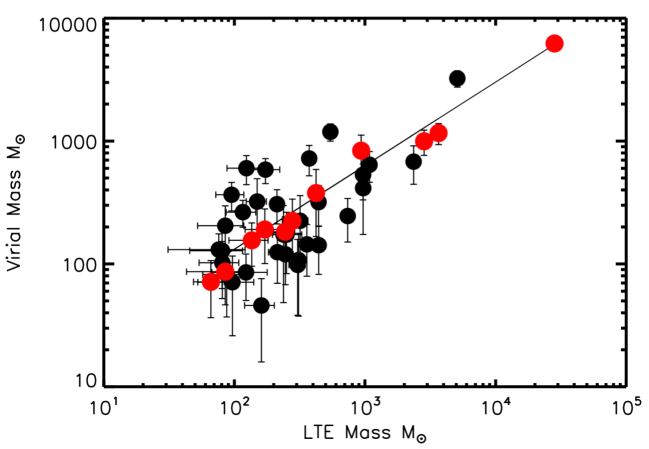
Figure 8: LTE mass versus virial mass relation of ¹³CO clumps (black) in N 55. Those with star formation (with YSOs) are shown in red for comparison.

7.2 Scaling relations

7.2.1 Size-linewidth relation

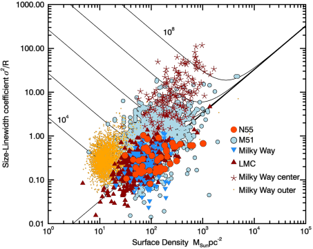
Figure 9: Size-linewidth coefficient $\sigma^{2}$/R is plotted against mass surface density in M_⊙ pc^-2 for N 55 ¹³CO(1-0) clumps. Milky Way GMCs (Heyer et al., 2009, 2001; Oka et al., 2001), M51 (Colombo et al., 2014) and the LMC molecular clouds from Mopra observations by Wong et al. (2011) are shown for comparison. The $\sigma^{2}$/R for N 55 clumps, Milky Way GMCs (Heyer et al., 2009) and the LMC clouds roughly show a linear relation to the mass surface density, indicating that clouds are virialized with negligible external pressure (along the solid diagonal line). The solid curves are pressure bounded virial equilibrium curves for external pressure ranging from $P$/k_B = 10⁴-10⁸ cm^-3K. The clouds in the Milky Way centre and Milky Way outer show large velocity dispersion and confined by external pressure.

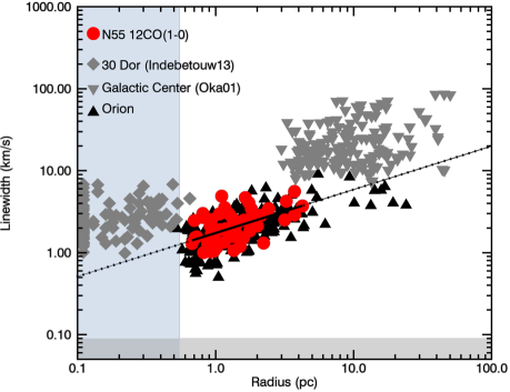
Figure 10: Linewidth versus radius relation for ¹²CO(1-0) in N 55 compared to that of Orion molecular cloud and 30 Doradus. The N 55 clumps follow a power law relation, $\Delta V\propto R^{0.5}$, which agrees well with the Orion clumps. The shaded blue indicates the region where the observational resolution affects the sizes.

In order to check the virial boundedness of the clumps we test the relationship between the mass surface density, size and linewidth of the clumps (Heyer et al., 2009), since the virial theorem links those three basic parameters. Leroy et al. (2015) have reported a diagnostic diagram relating the size-linewidth coefficient $\sigma_{v}^{2}$/$R$ with mass surface density to distinguish the pressure-bound clouds from gravity-bound. For this relation, the mass surface density is obtained from the LTE assumption. In figure 9 we show the $\sigma_{v}^{2}$/$R$ - surface density relation for N 55 ¹³CO(1-0) clumps, where the mass densities are derived from the LTE assumption. For comparison we show the Milky Way clouds (Heyer et al., 2009) which are observed with spatial scale $3.5-13$ pc and spectral resolution 1 km s^-1, the Milky Way center clouds (Oka et al., 2001) observed with 1.4 pc spatial and 2 km s^-1 spectral resolutions, the Milky Way outer clouds (Heyer et al., 2001) observed with $0.4-4.5$ pc spatial and 0.98 km s^-1 spectral resolutions, M51 clouds (Colombo et al., 2014) observed with 40 pc spatial and 5 km s^-1 spectral resolution, and the LMC clouds from ¹²CO(1-0) Mopra survey (Wong et al., 2011) with 14.5 pc spatial and 0.5 km s^-1 spectral resolutions. The solid curves are $\sigma_{v}^{2}$/$R$ as a function of surface density for a range of external pressures 10⁴–10⁸ cm^-3 K (Field et al., 2011). $\sigma_{v}^{2}$/$R$ roughly shows a linear relation with mass surface density for N55 clumps, many Milky Way GMCs and the LMC clouds, while the Milky Way center and outer clouds show deviation from the linear trend. If the clouds are in virial equilibrium, i.e. with low external pressure, the velocity dispersion of these clouds can be determined from their mass surface density. This relation is shown by a diagonal solid line in Figure 9, where the mass surface density $\sim$ 330$\sigma^{2}$/$R$. This relation indicates that N 55 clumps are virialized with negligible external pressure. In Figure 10, we compares the linewidth (2$\sqrt{2{\rm ln}2}\times$velocity dispersion) versus radius relation for ¹²CO(1-0) clumps (dendrogram trunks) in N 55 with Orion, 30 Doradus and Galactic center clouds. For Orion molecular cloud, ¹²CO(1-0) data of Dame et al. (2001) was decomposed with astrodendro as for N 55 clumps. The 30 Doradus size-linewidth relation is shown for the ¹²CO(2-1) transition derived by Indebetouw et al. (2013). The radius-linewidth relation for N 55 is fitted with a function $\Delta V$ $\propto\,R^{0.5}$ with a correlation coefficient of 0.7. This relation agrees well with the Orion molecular cloud. The 30 Doradus and Galactic center clouds show larger velocity dispersions compared to N 55 and Orion.

7.2.2 Virial mass-luminosity relation

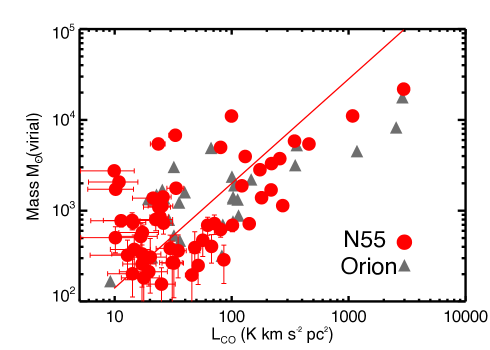
Figure 11: Virial mass versus luminosity relation for ¹²CO(1-0) clumps in N 55 is fitted with a function log($M_{{\rm VIR}}$)=1.0+(1.15$\pm$0.3) log($L_{{\rm co}}$) for a correlation coefficient 0.6. For a comparison, the virial mass versus luminosity relation for Orion is shown.

The Galactic molecular clouds and low-resolution ¹²CO(1-0) observation of the LMC molecular clouds show a power law correlation between ¹²CO luminosity and virial mass. Solomon et al. (1987) demonstrated how to use the mass-luminosity relation of optically thick ¹²CO(1-0) lines as a calibrator for total cloud mass, i.e. molecular hydrogen mass. They found a tight correlation between ¹²CO(1-0) luminosity and virial mass with a power law index of 0.81 for nearly 278 Galactic molecular clouds. Figure 11 compares the virial mass versus the ¹²CO(1-0) luminosity relation of N 55 clumps with the Orion molecular cloud obtained with the NANTEN 4 m telescope (Nishimura et al., 2015). The N 55 clouds show a power law relation between virial mass and CO luminosity (correlation coefficient 0.6) with a scatter of more than an order of magnitude. The mass-luminosity relation of N 55 in Figure 11 is fitted with a function log($M$)=($1.15\pm 0.3$) log($L_{\rm CO})+1.0$. The Orion cloud shows a power law index of 0.55.

7.3 Cloud mass spectrum

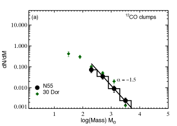
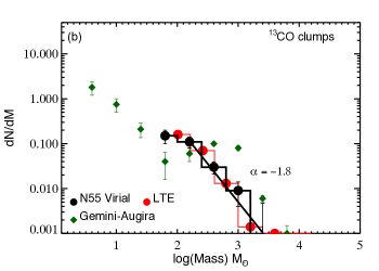
Figure 12: The ¹²CO(1-0) and ¹³CO(1-0) clump mass spectra obtained from dendrogram trunks are shown in (a) and (b) respectively. The masses are derived from the virial and LTE assumptions. The best fit power-law index for the function $dN/dM\propto M^{-\alpha}$ is $1.5\pm 0.15$ for ¹²CO(1-0) and $1.8\pm 0.25$ for ¹³CO(1-0). For comparison, the clump mass spectra of 30 Doradus (Indebetouw et al., 2013) and Gemini-augira clouds (Kawamura et al., 1998) are given.

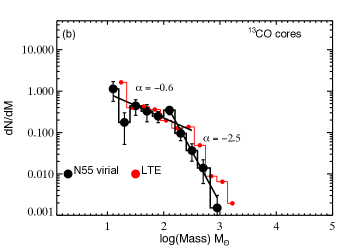
Figure 13: The ¹²CO(1-0) and ¹³CO(1-0) core mass spectra obtained from dendrogram leaves are given in (a) and (b) respectively. a) The best fit power-law index for ¹²CO(1-0) in low-mass end is $\alpha$=$0.5\pm 0.05$, and in high-mass end $\alpha$=$2.0\pm 0.3$. b) The best fit power-law index for the ¹³CO(1-0) core mass spectrum is $0.6\pm 0.2$ in low-mass end, and $2.5\pm 0.4$ in high-mass end.

The mass spectrum of a distribution of molecular clumps in a cloud is usually represented in a differential form of cloud numbers N_i in the mass range between $M_{i}$ and $M_{i}+dM$, where $dM$ is mass bin. This can be represented as $dN/dM=f(M)$. It is found that the molecular cloud mass spectrum is often well described by a power law:

$$\frac{dN}{dM}\propto M^{-\alpha}$$ (6)

The above differential form of the power law can be sensitive to the adopted mass bins, hence a cumulative or a truncated power law is often adopted to represent the mass distribution, $dN/d{\rm ln}M\propto(M_{m}/M)^{\alpha}$ (Kawamura et al., 1998; Indebetouw et al., 2013). Here $dN$ is the number of clouds in the mass range $M_{i}$ and $M_{i}+d{\rm ln}M$, and $M_{m}$ is the upper mass. However, it is much easier to recognize the behavior of a mass spectrum in differential form, as in equation 6. Therefore, in our analysis we use the differential form of clump mass spectrum i.e. $dN/dM=f(M)$. We find that index of the power law is not affected by the mass bins we adopted.

From the dendrogram analysis of ¹²CO(1-0) and ¹³CO(1-0) maps, we have obtained two sets of structures, molecular cores (leaves) and clumps (trunks). We use these leaves and trunks separately to construct the mass spectra and compare their trends in Figures 12 and 13. We compare the mass spectra of N 55 from the virial as well as LTE masses calculated for ¹²CO(1-0) and ¹³CO(1-0). The trunks reveal the high mass end of mass spectra in both ¹²CO(1-0) and ¹³CO(1-0) which are fitted with the functions $dN/dM\propto M^{-1.5\pm 0.15}$ and $dN/dM\propto M^{-1.8\pm 0.25}$ respectively. In Figure 12 a, for comparison we show the mass spectrum of the star-forming region 30 Doradus in the LMC from ¹²CO(2-1) clumps observed with ALMA (Indebetouw et al., 2013) along with the ¹²CO(1-0) clump mass spectrum in N 55. In Figure 12 b, we present the clump mass spectrum for ¹³CO(1-0), and compare the power law behavior with Gemini-Augira cloud (in the same mass range 10-10⁴M _⊙) in the Milky Way (Kawamura et al., 1998). The dendrogram leaves are tracers of the low-mass cores along with a few high-mass cores which clearly show a turnover below 200 M_⊙ (Figure 13) in the mass spectrum. The low-mass end of ¹²CO(1-0) mass spectrum, $\leq$ 200 M_⊙, is fitted with a power law index of 0.5$\pm$0.1 and that for ¹³CO(1-0) is fitted with a power law index of 0.6$\pm$0.2. The steep high-mass part shows power law indices 2.0$\pm$0.3 and 2.5$\pm$0.4 for ¹²CO(1-0) and ¹³CO(1-0) cores respectively.

8 Discussion

8.1 Clump physical properties: size-linewidth relation and mass spectrum

We quantify the molecular clump properties at smaller scales (sub-parsec $\sim$0.1 pc) and probe the GMC characteristics’ close relationship to star formation in N 55 using ALMA observations. In order to investigate, how the N 55 GMC properties differ from those of the Galaxy, we compare the size-linewidth, virial mass-luminosity and clump mass function relations of clouds in N 55 with the Orion molecular cloud, Milky Way outer and inner clouds and Gemini-Augira regions (Figures 10 - 13). As we have already noted in section 1, the Galactic molecular clouds and many extragalactic clouds which are observed at resolutions of $>$10 pc show a power law relation between clump size and velocity dispersion $\sigma_{v}$: $\sigma_{v}\propto R^{\beta}$. Does this size-linewidth power law relation hold or breakdown in sub-parsec scales for the LMC? Do we find any deviation in size-linewidth power law behavior at lower metallicity, where the clumps can be highly dissociated by hard UV radiation or perturbed by shocks due to massive star formation?

Indebetouw et al. (2013) and Nayak et al. (2016) have reported cloud properties of 30 Doradus using ¹²CO(2-1) observations with ALMA. They noticed a large scatter in the size-linewidth relation with relatively high velocity dispersion in 30 Doradus compared to the Galactic clouds, indicating the effect of external pressure in addition to gravitational equilibrium. This behavior can be checked in other star-forming regions in the LMC. The size-linewidth relation in Figure 10 indicates that the N 55 molecular clumps show very similar power law relationship as in the Orion cloud. The Galactic center and 30 Doradus clouds show large velocity dispersions which the authors say may be due to the effect of external pressure. In Figure 9, we try to evaluate whether any effect of external force is required for equilibrium confinement of N 55 molecular clumps in addition to gravity. Like many Milky Way GMCs and the LMC molecular clouds from the Mopra survey, the N 55 clouds reported in this work cluster around the equilibrium line (solid diagonal line in Figure 9) as defined by Leroy et al. (2015). This relation suggests that N 55 clumps are gravitationally bound. Clouds clustering above this line include GMCs in the outer and center regions of the Milky Way, which require high external pressure for confinement in a high turbulent medium. We note that in N 55 clouds the average ratio of virial mass to LTE mass is 1.12, where the LTE mass versus virial mass relation is fitted with a power law index 0.68$\pm$0.12 which is consistent with the power index found for Orion cloud (i.e. gravitationally bound) (Ikeda & Kitamura, 2009; Liu et al., 2012).

The core mass distribution is another important characteristic of the molecular cloud population which has a significant impact on star-forming clouds, because of its similarity with the stellar initial mass function. For the inner Milky Way clouds, the mass distribution follows a power law relation $dN/dM\propto M^{-\alpha}$ where $\alpha=1.5$. The surveys of the Local Group galaxies have revealed the power law behavior of cloud mass spectrum (Wong et al., 2011). The clump mass spectrum of N 55 tends to follow a similar behavior as in 30 Doradus of the LMC, Gemini-Augira cloud, and many other star-forming clouds in the Milky Way. We note that ALMA observation of ¹²CO(1-0) and ¹³CO(1-0) emission in N 55 reveal more massive clumps than in 30 Doradus by ¹²CO(2-1) emission. This may be due to the hard radiation field and preferential destruction of molecular clumps in 30 Doradus. Kawamura et al. (1998) reported a power law index of 1.4–1.9 for Gemini-Augira clouds. Similar studies have been done for Cepheus and Cassiopeia regions with the ¹³CO(1-0) survey by Yonekura et al. (1997). They have compared the mass spectrum behavior of Cepheus and Cassiopeia with several other ¹³CO Galactic clouds and reported a power law index in the range of 1.5–1.8 for most of the ¹³CO clouds with the mass range 10–10⁵M_⊙. This power law behavior of the clump mass spectrum is consistent with many star-forming clouds in the Milky Way, such as Orion (Ikeda et al., 2009; Johnstone et al., 2000, 2006), $\rho$Ophiuchi cloud (Motte et al., 1998), and Taurus (Onishi et al., 2002). These studies have shown the power law index of 2.0–3.0 in the high-mass part. Our studies show that the mass spectrum index is not dependent on the environments sampled. This study confirms a universal behavior of the clump mass function at smaller spatial scales in a sub-solar metallicity galaxy.

8.2 X_CO factor

We determine the CO-to-H₂ conversion factor for N 55 molecular clouds using our ¹²CO(1-0) observations. Since the determination of molecular hydrogen mass is fundamental to understand the physics of star formation, and a direct detection of bulk H₂ mass is almost impossible, the CO luminosity-mass relation is widely used as a calibrator for measuring the CO-to-H₂ mass conversion factor, X_CO (Solomon et al., 1987). The reason for using the CO luminosity-mass relation as a calibrator for X_CO is that, for gravitationally bound clouds the ratio of virial mass to ¹²CO luminosity is directly proportional to the square root of H₂ density and inversely proportional to the average brightness temperature (Solomon & Barrett, 1991). In our analysis, the masses of N 55 clumps are determined by LTE and virial assumption of ¹²CO and ¹³CO emission. The consistency between LTE mass and virial mass of the clumps along with a virial ratio of 1.12, and the virial equilibrium relationship in the $\sigma^{2}$/R versus mass surface density plot (where the mass surface density is determined using the LTE method) strongly suggest that N 55 clumps are gravitationally bound. Fukui et al. (2008) reported a power law relation between ¹²CO(1-0) luminosity and virial mass with an index of 1.2$\pm$0.3 for the LMC molecular clouds. This relation yields an X_CO factor of 7$\times$10²⁰ cm^-2(K km s^-1)^-1 for a total cloud mass of 28$\times$10⁵ M_⊙ and luminosity 2$\times$ 10⁵ K km s^-1 pc² using the NANTEN CO survey. Note that the NANTEN CO survey of the LMC has a spatial resolution of 2.6${}^{\prime}\sim$ 37 pc. Using the Mopra CO data of the LMC at spatial resolution 45${}^{\prime\prime}\sim$ 11 pc, the value of X_CO is reported to be 4$\times$10²⁰ cm^-2(K km s^-1)^-1 (Hughes et al., 2010). The virial mass-luminosity relation of N 55 is fitted with a power law index of 1.15$\pm$0.3 (Figure 11). This relation yields an X_CO factor 6.5$\times$10²⁰ cm^-2(K km s^-1)^-1 for a total cloud mass of 1.2$\times$ 10⁵ M_⊙ and luminosity of 8$\times$ 10³K km s^-1 pc². This X_CO factor value is consistent with the value given in Fukui et al. (2008). In Figure 11, we compare the mass-luminosity relation of the N 55 clumps with that of Orion cloud. The mass-luminosity relation of the Orion cloud yields an X_CO factor comparable to that found for Galactic clouds (Polk et al., 1988).

8.3 Star formation

In order to investigate the efficiency with which the stars form within the dense cores, we adopt the YSOs identified from Spitzer and Herschel observations. In section 7.1 we compare the physical properties of the star-forming CO cores with the non-star-forming CO cores. We compare the histograms of radius, velocity width, and mass of ¹³CO and ¹²CO cores. The star-forming CO cores tend to have larger masses compared with the non-star-forming cores. The velocity widths of the ¹³CO and ¹²CO cores also show a similar trend, where the star-forming cores have a velocity width larger than the critical velocity width. This may indicate some effect of turbulence. This result is consistent with the study of ¹³CO clumps in 30 Doradus, where the massive star formation occurs in clumps with high masses and linewidths (Nayak et al., 2016). The size-linewidth relation of N 55 indicates a negligible effect of external pressure, hence the larger velocity width of star-forming clouds might be due to high radiation fields or shocks caused by nearby massive stars. These findings are consistent with massive star forming regions in Galactic clouds such as Orion molecular cloud (Ikeda et al., 2009) and Gemini-Augira cloud (Kawamura et al., 1998).

Gruendl & Chu (2009) and Seale et al. (2014) identified about 16 young stellar objects in N 55 using infrared colors. Among them, 15 are in the field of our ALMA observation. From Gruendl & Chu (2009) we obtained Spitzer photometric magnitudes of seven YSOs. However, we do not have enough parametric information, such as mass and luminosities for a detailed study of star formation efficiency. Gruendl & Chu (2009) suggested a selection criterion 8.0${\,\rm\mu m}$ $\leq$ [8.0] for massive YSOs in the LMC. This can be a reasonable approximation for estimating the masses, even though a strict mass-luminosity relation is not valid. The infrared spectral energy distribution fitting of the YSOs in N 44 and N 159 of the LMC have shown that, the brightest YSOs with 8.0${\,\rm\mu m}$ magnitude $\leq$ [8.0] have masses $\geq$ 8.0M_⊙ (Chen et al., 2009, 2010). The brightest source identified with Spitzer in our field of observation has a 8.0${\,\rm\mu m}$ magnitude of [7.27$\pm$0.07] which can have a mass of 20M_⊙ and a luminosity of 6.0$\times$10⁴ L_⊙ according to Chen et al. (2009) (Table 7). Three sources have 8.0${\,\rm\mu m}$ magnitudes $\sim$ [8.76, 8.94, 8.24] which represent masses in the range 8–15 M_⊙, and two others show 8.0${\,\rm\mu m}$ magnitude $\sim$ [10.17, 10.49] which may have masses below 8.0M_⊙. These studies indicate that N 55 is a site for high and intermediate mass star formation in the LMC.

Table 2: Position of identified YSOs and associated clumps

Number	Identified YSOs		Associated Clumps		cClump ID
	R.A. (deg)	Decl. (deg)	R.A. (deg)	Decl. (deg)
1a	083.0245	-66.4252	83.0270	-66.4258	23
2	083.0936	-66.4601	83.0936	-66.4602	53
3	083.0946	-66.4523	83.0949	-66.4523	33
4	083.1076	-66.4860	83.1077	-66.4858	37
5	083.1335	-66.4542	83.1352	-66.4547	77
6	083.1371	-66.4526	83.1372	-66.4524	38
			83.1374	-66.4563	2
			83.1404	-66.4550	55
7	083.0357	-66.3870	83.0342	-66.3869	98*
8b	082.9186	-66.4311	82.9227	-66.4325	4
9	083.0024	-66.4206	82.9999	-66.4202	72
			83.0045	-66.4207	66
10	82.9945	-66.4267	82.9923	-66.4275	91*
11	82.9977	-66.4287	82.9923	-66.4275
12	83.0428	-66.4134	83.0435	-66.4139	28
13	83.0462	-66.4151	83.0486	-66.4152	5
14	82.9979	-66.4635	83.0581	-66.4684	125*
15	83.1578	-66.4699	83.1581	-66.4703	10

a: Spitzer YSOs from Gruendl & Chu (2009). b: Herschel YSOs from Seale et al. (2014). c: ¹³CO clump number IDs from Table 5; those with * are identified in ¹²CO emission (Table 3, 6), but not in ¹³CO.

9 Summary

We report the molecular cloud properties of the N 55 star forming region in the LMC with ALMA observations of ¹²CO(1-0) and ¹³CO(1-0) emission. This cloud is strongly irradiated by a young star cluster LH 72 within an expanding SGS, LMC 4. The results of our analysis are summarized as follow:

1. ALMA observations of N 55 reveal the clumpy nature of CO clouds in sub-parsec scales. The cloud properties are analyzed using dendrograms which give two sets of clumps, leaves and trunks. We use both leaves and trunks separately to understand their physical properties such as radii, linewidths, luminosities, masses, and their relation to star formation. We find that molecular cores (dendrogram leaves) that are associated with YSOs generally show larger linewidths and masses.

2. The ¹²CO and ¹³CO clump masses are determined by LTE and virial assumptions. These independent mass estimates show that the LTE masses of most of the clumps are in very good agreement with the virial masses, and the LTE versus virial mass plot can be fitted with a power law of $M_{{\rm VIR}}$=1.75$M_{{\rm LTE}}^{0.68\pm 0.12}$, where the virial ratio is 1.12. The size-linewidth coefficient ($\sigma^{2}$/R) shows a linear relation with mass surface density as in many Milky Way and LMC quiescent clouds, where mass surface density is determined by LTE method. These findings indicate that N 55 clumps are in self-gravitational virial equilibrium with negligible external pressure.

3. The size-linewidth relation is a power law with an index of 0.5$\pm$0.05, which is consistent with the the size-linewidth relation of the Orion cloud, measured at similar spatial scale. This result strengthens our argument that N 55 clouds are gravitationally bound and the effects of any external pressure can be negligible. We present the size-linewidth relation of ¹²CO clumps that are identified as dendrogram trunks whose power law relation does not show much difference from ¹³CO clumps.

4. A power law relation between ¹²CO virial mass and luminosity is presented, which gives an X_CO factor of 6.5$\times$ 10²⁰ cm^-2 (K km s^-1)^-1. This value of X_CO factor is two times the value of Orion cloud, measured for similar spatial scale.

5. ¹²CO and ¹³CO core mass functions show a turnover below 200M_⊙. This turnover separates the steep high mass end from the shallower low-mass part. The low-mass end of the ¹²CO mass spectrum is fitted with a power law of index 0.5$\pm$0.1, while for ¹³CO it is fitted with a power law index 0.6$\pm$0.2. The steep high-mass end is fitted with a power law index 2.0$\pm$0.3 for ¹³CO clumps and 2.5$\pm$0.4 for ¹³CO. Our studies show that clump mass function in N 55 shows trend similar to Galactic clouds.

Table 3: ¹²CO(1-0) clump (dendrogram trunks) properties

Number ID	R.A.	Decl.	Radius (R)	$\delta$R	$\sigma_{v}$	$\delta\sigma_{v}$	Velocity	Lco(K km s-1 pc2)		Tpk	MVIR	$\delta$M
	deg	deg	pc	pc	km s-1	km s-1	km s-1	$\delta$Lco	$\delta$Lco	K	M⊙	M⊙
1	83.1367	-66.4543	3.73	0.12	2.37	0.10	288.9	2958	2.0	40.0	21824	40
2	83.1385	-66.4603	0.80	0.50	1.14	0.50	276.3	23.8	6.2	9.1	1095	210
3	83.0718	-66.4039	1.79	0.23	0.86	0.25	283.3	180.2	3.3	22.1	1389	120
4	83.0535	-66.4027	0.94	0.50	1.08	0.45	283.7	25.3	6.0	10.2	1128	200
5	82.9232	-66.4267	0.96	0.40	0.602	0.42	283.7	34.9	6.0	10.1	362	180
6	83.0545	-66.4130	4.26	0.10	1.58	0.10	287.5	1082.5	1.4	25.3	11057	45
7	82.9230	-66.4328	0.98	0.35	0.446	0.30	283.7	14.2	5.5	6.9	202	90
8	83.0979	-66.4531	2.42	0.16	1.47	0.20	289.4	458.1	2.7	30.2	5431	100
9	83.0895	-66.4777	1.43	0.35	0.97	0.30	285.9	25.9	4.5	9.7	1416	120
10	83.1581	-66.4704	1.07	0.38	1.26	0.35	286.0	33.4	5.5	10.2	1768	135
11	83.1484	-66.4608	0.71	0.50	0.647	0.50	284.5	20.1	7.5	11.4	309	185
12	83.0427	-66.4036	1.82	0.24	1.45	0.23	287.4	130.6	3.2	21.6	3954	100
13	82.9686	-66.4181	0.90	0.50	0.46	0.40	284.8	45.7	5.5	28.2	196	150
14	83.1073	-66.4855	1.11	0.43	2.08	0.35	288.5	80.4	8.0	20.2	4983	140
15	83.0609	-66.4384	0.81	0.40	1.28	0.45	286.7	21.3	7.0	10.4	1374	170
16	83.0404	-66.4313	1.01	0.47	0.49	0.30	286.2	51.7	4.8	19.5	249	95
17	83.0547	-66.4403	0.70	0.40	1.05	0.52	286.5	22.4	9.0	11.4	800	200
18	82.9795	-66.4054	3.73	0.12	1.23	0.12	287.9	344.7	1.6	17.1	5841	55
19	83.0581	-66.4685	0.98	0.30	0.61	0.40	286.1	14.7	5.5	8.8	374	165
20	83.1569	-66.4448	1.77	0.30	0.79	0.25	287.6	273.2	3.5	24.1	1137	125
21	83.0753	-66.4467	3.16	0.14	1.07	0.10	288.2	258.0	1.4	13.2	3744	40
22	83.0266	-66.4012	2.01	0.18	0.90	0.20	287.3	217.3	3.0	20.9	1693	85
23	83.0343	-66.3870	0.73	0.40	0.66	0.50	286.3	17.1	7.7	13.4	334	190
24	83.0904	-66.4605	2.14	0.20	1.22	0.20	289.1	219.2	3.0	26.7	3302	90
25	83.1245	-66.4425	1.64	0.25	1.99	0.27	289.6	32.9	4.0	3.3	6775	125
26	83.1510	-66.4679	1.74	0.28	1.73	0.25	288.9	23.6	3.4	2.6	5436	115
27	83.1618	-66.4544	3.25	0.12	1.80	0.13	288.5	99.6	1.8	4.3	11030	60
28	83.1155	-66.4536	1.25	0.38	1.26	0.30	287.5	10.9	5.0	3.0	2068	120
29	83.0712	-66.4402	0.97	0.40	0.50	0.40	286.8	17.1	5.5	15.3	259	160
30	83.1090	-66.4331	0.93	0.40	0.73	0.45	287.3	16.7	6.5	5.4	521	205
31	82.9541	-66.4189	0.95	0.40	0.76	0.35	286.9	17.2	6.5	6.5	576	120
32	82.9657	-66.4131	1.38	0.25	0.71	0.35	287.4	71.2	4.0	16.2	722	175
33	83.1181	-66.4829	1.60	0.30	1.06	0.24	288.5	122.2	3.7	18.3	1881	100
34	83.0252	-66.4273	2.23	0.20	0.56	0.18	287.2	141.3	2.6	16.4	719	75
35	83.0171	-66.4489	1.32	0.28	0.67	0.28	287.8	80.5	4.0	23.1	620	110
36	82.9924	-66.4275	0.67	0.40	0.55	0.30	287.2	19.6	9.0	14.9	213	65
37	82.9958	-66.4127	0.82	0.40	0.43	0.30	286.8	25.1	7.8	14.6	155	80
38	83.0639	-66.4578	0.95	0.30	0.69	0.40	288.3	56.6	5.5	18.0	473	160
39	83.1261	-66.4460	1.16	0.40	1.51	0.30	288.9	9.9	4.8	3.9	2747	110
40	83.1401	-66.4429	1.22	0.33	0.781	0.30	287.4	11.3	5.0	3.3	775	115

Table 3: Continued

Number ID	R.A.	Decl.	Radius (R)	$\delta$R	$\sigma_{v}$	$\delta\sigma_{v}$	Velocity	Lco(K km s-1 pc2)		Tpk	MVIR	$\delta$M
	deg	deg	pc	pc	km s-1	km s-1	km s-1	$\delta$Lco	$\delta$Lco	K	M⊙	M⊙
41	83.1110	-66.4432	1.33	0.30	1.12	0.25	288.6	10.2	4.3	3.6	1724	90
42	83.1417	-66.4321	1.16	0.40	0.57	0.40	288.0	48.4	4.6	19.7	392	195
43	82.9530	-66.4161	0.94	0.30	0.52	0.40	287.6	32.0	6.7	17.9	265	155
44	83.0357	-66.4396	0.94	0.43	0.72	0.40	288.0	10.1	5.0	5.3	505	160
45	83.0006	-66.4211	1.85	0.20	1.21	0.23	290.5	174.5	2.8	19.4	2827	100
46	83.0744	-66.4120	1.43	0.27	0.70	0.29	289.3	14.3	4.1	5.8	740	125
47	83.0312	-66.4501	1.60	0.30	0.65	0.25	289.3	101.5	3.5	22.8	692	105
48	83.0659	-66.4510	0.88	0.44	0.59	0.40	289.6	12.9	6.7	6.5	324	150
49	83.0189	-66.3943	1.18	0.35	0.83	0.30	290.2	24.4	4.4	7.2	855	110
50	83.1110	-66.4782	1.50	0.27	0.51	0.30	289.9	67.2	4.2	20.6	404	140
51	83.1126	-66.4494	0.92	0.50	0.44	0.35	290.0	17.7	6.3	12.5	182	117
52	83.0756	-66.4370	1.38	0.33	0.70	0.33	290.3	62.4	3.8	16.1	692	155
53	83.1202	-66.4722	1.35	0.28	0.45	0.30	290.6	85.7	4.0	22.2	288	130
54	83.1452	-66.4441	0.92	0.48	0.63	0.40	290.8	29.8	7.2	13.5	385	153
55	83.1504	-66.4502	1.07	0.33	0.81	0.40	291.1	26.1	5.2	4.5	729	177
56	83.0355	-66.4186	0.91	0.50	0.91	0.42	293.2	14.1	6.0	4.5	781	167
57	83.0286	-66.4206	0.88	0.50	0.54	0.46	293.7	31.0	6.8	21.3	268	195

Table 4: ¹³CO(1-0) clump (dendrogram trunks) properties

Number ID	R.A.	Decl.	Radius (R)	$\delta$R	$\sigma_{v}$	$\delta\sigma_{v}$	Velocity	Tpk	Lco  (K km s-1 pc2)		N${}_{\rm H_{2}}$	MLTE	$\delta$MLTE	MVIR	$\delta$M
	deg	dec	pc	pc	km s-1	km s-1	km s-1	K	$\delta$Lco	$\delta$Lco	1021cm-2	M⊙	M⊙	M⊙	M⊙
1	83.1354	-66.4586	0.55	0.30	0.58	0.40	282.0	1.99	1.7	0.5	4.0	171	50	191	90
2	83.0713	-66.4044	1.23	0.35	0.65	0.40	283.1	1.38	9.5	0.2	5.0	967	23	532	200
3	83.1374	-66.4563	0.65	0.30	0.48	0.30	282.8	1.15	1.3	0.4	2.9	136	45	156	60
4	82.9227	-66.4325	0.80	0.40	0.29	0.20	283.5	1.96	1.1	0.3	1.0	66	20	72	35
5	83.0486	-66.4152	0.63	0.30	0.53	0.30	284.8	2.16	2.4	0.5	3.8	245	45	183	60
6	83.0623	-66.4126	2.33	0.20	1.16	0.45	287.2	3.77	40	0.1	9.9	5097	15	3237	490
7	83.1374	-66.4539	2.98	0.15	1.42	0.42	288.9	5.39	154	0.1	27	28278	20	6222	550
8	82.9683	-66.4180	0.73	0.40	0.36	0.28	284.9	2.74	2.3	0.3	4.4	305	45	98	60
9	82.9886	-66.4064	0.55	0.30	0.39	0.25	286.4	1.94	1.2	0.5	3.3	123	55	85	35
10	83.0404	-66.4313	0.88	0.40	0.39	0.25	286.2	3.03	4.1	0.3	4.1	443	34	142	60
11	83.1567	-66.4451	1.55	0.30	0.65	0.38	287.6	4.20	19.3	0.2	8.5	2357	20	680	235
12	82.9783	-66.4053	1.04	0.40	0.55	0.40	287.1	1.72	1.6	0.3	1.7	149	25	322	172
13	82.9644	-66.4129	0.75	0.40	0.88	0.45	287.3	0.94	1.4	0.4	2.0	124	35	602	160
14	83.0264	-66.4017	1.44	0.30	0.53	0.40	287.2	1.91	9.7	0.2	4.8	969	25	414	240
15	82.9956	-66.4127	0.69	0.35	0.31	0.25	286.7	1.54	1.1	0.5	1.8	97	44	71	45
16	83.1187	-66.4828	1.20	0.35	0.76	0.40	288.2	1.52	4.0	0.2	2.9	374	22	722	200
17	83.0953	-66.4526	1.36	0.40	0.91	0.40	288.8	6.58	23.0	0.2	14	3662	30	1162	225
18	83.0642	-66.4441	0.81	0.40	0.52	0.40	287.3	3.11	2.6	0.4	3.8	319	47	225	135
19	82.9715	-66.4041	0.61	0.30	0.57	0.38	287.3	1.10	1.0	0.4	1.9	85	33	205	92
20	83.0251	-66.4268	1.65	0.28	0.47	0.35	287.3	1.29	4.5	0.2	2.3	422	18	377	210
21	83.0435	-66.4136	1.25	0.30	0.87	0.42	288.6	3.80	19.0	0.2	13	2835	30	995	230
22	83.1243	-66.4558	0.54	0.30	0.55	0.40	287.6	2.47	2.2	0.7	5.6	251	78	173	90
23	83.0425	-66.4038	0.81	0.40	0.83	0.40	288.3	1.13	1.7	0.5	2.2	173	50	586	135
24	83.0930	-66.4601	1.08	0.40	0.86	0.50	289.2	2.73	7.0	0.3	6.7	936	40	836	280
25	83.0640	-66.4576	0.75	0.40	0.47	0.40	288.4	2.25	2.4	0.4	3.2	238	40	173	125
26	82.9536	-66.4163	0.67	0.32	0.43	0.30	287.8	1.08	0.9	0.4	1.5	81	35	128	65
27	83.1077	-66.4858	0.67	0.32	0.57	0.40	289.4	2.32	2.4	0.4	4.1	278	45	225	112
28	83.0165	-66.4488	0.85	0.40	0.37	0.25	288.2	1.80	2.0	0.3	2.4	214	30	125	55
29	83.0813	-66.4489	1.00	0.52	0.48	0.30	288.9	2.77	5.7	0.3	5.7	738	35	246	95
30	83.1419	-66.4321	0.80	0.40	0.38	0.25	288.2	2.49	2.4	0.4	3.1	246	35	120	52
31	83.0466	-66.4090	0.53	0.30	0.49	0.28	288.3	1.28	0.9	0.6	2.1	76	45	131	45
32	83.0714	-66.4469	0.99	0.40	0.55	0.30	288.8	1.57	2.5	0.3	2.2	212	22	307	95
33	83.0312	-66.4501	1.41	0.32	0.47	0.28	289.4	2.35	3.7	0.2	3.1	441	25	319	115

Table 4: Continued

Number ID	R.A.	Decl.	Radius (R)	$\delta$R	$\sigma_{v}$	$\delta\sigma_{v}$	Velocity	Tpk	Lco  (K km s-1 pc2)		N${}_{\rm H_{2}}$	MLTE	$\delta$M	MVIR	$\delta$M
	deg	dec	pc	pc	km s-1	km s-1	km s-1	K		$\delta$Lco	1021cm-2	M⊙	M⊙	M⊙	M⊙
34	82.9848	-66.4055	0.97	0.45	0.38	0.25	289.2	2.86	3.5	0.3	3.2	359	28	144	65
35	82.9704	-66.4098	0.72	0.35	0.37	0.25	289.3	1.60	1.0	0.3	1.6	81	27	102	50
36	83.1375	-66.4616	0.97	0.45	0.80	0.42	290.3	3.79	6.8	0.4	7.6	1083	62	642	180
37	83.0014	-66.4205	1.11	0.43	1.01	0.40	290.5	2.59	5.5	0.2	4.0	544	24	1188	190
38	83.0770	-66.4365	0.68	0.37	0.61	0.30	290.2	1.40	1.3	0.3	2.2	116	30	264	65
39	82.9953	-66.4220	0.64	0.30	0.36	0.25	290.2	1.82	1.0	0.5	1.9	85	42	86	40
40	83.1098	-66.4774	0.73	0.35	0.25	0.20	290.2	2.10	1.5	0.4	2.5	161	41	46	30
41	83.1210	-66.4716	0.82	0.40	0.36	0.28	290.5	2.45	2.5	0.4	3.6	310	46	108	70
42	83.1453	-66.4443	0.69	0.30	0.34	0.25	290.9	1.80	1.1	0.4	1.8	87	30	82	45
43	83.1079	-66.4542	0.99	0.45	0.60	0.30	291.4	0.93	1.2	0.3	1.3	95	23	365	95

Table 5: ¹³CO(1-0) core (dendrogram leaves) properties

Number ID	R.A.	Decl.	Radius	$\sigma_{v}$	Velocity	Tpk	Lco	MLTE	MVIR
	deg	dec	pc	km s-1	km s-1	K	K km s-1 pc2	M⊙	M⊙
1	83.1354	-66.4586	0.55	0.58	282.0	2.0	1.7	160	191
2	83.1374	-66.4563	0.65	0.48	282.8	1.2	1.3	135	156
3	83.0712	-66.4042	0.76	0.43	283.2	1.6	3.1	312	145
4	82.9227	-66.4325	0.80	0.29	283.6	1.4	1.1	62	71
5	83.0486	-66.4152	0.63	0.53	284.8	2.2	2.4	245	183
6	82.9683	-66.418	0.73	0.36	284.9	2.7	2.3	305	98
7	83.1357	-66.4546	0.59	0.14	284.9	4.4	0.2	41	13
8	83.0605	-66.4122	1.14	0.57	286.2	3.1	7.7	973	386
9	82.9886	-66.4064	0.55	0.39	286.4	1.9	1.2	123	85
10	83.1449	-66.455	0.66	0.28	285.8	1.9	1.2	112	54
11	83.0411	-66.4317	0.46	0.23	286.0	3.0	1.3	137	26
12	82.9644	-66.4129	0.75	0.88	287.3	0.9	1.4	125	602
13	83.0594	-66.4094	0.81	0.43	286.5	1.8	2.5	216	153
14	82.9956	-66.4127	0.69	0.31	286.8	1.5	1.1	97	71
15	83.1187	-66.4828	1.20	0.76	288.2	1.5	4.0	374	722
16	83.0642	-66.4441	0.81	0.52	287.3	2.8	2.6	317	225
17	83.0226	-66.4281	1.01	0.36	287.2	1.0	1.6	128	136
18	82.9715	-66.4041	0.61	0.57	287.3	1.1	1.0	85	205
19	83.1243	-66.4558	0.54	0.55	287.6	2.5	2.2	251	173
20	83.027	-66.4258	0.88	0.41	287.1	1.8	2.0	189	153
21	82.9772	-66.4049	0.62	0.29	287.2	1.1	0.7	60	52
22	83.0278	-66.4023	0.60	0.34	287.1	2.1	1.2	123	74
23	83.0239	-66.4001	0.56	0.47	287.3	3.5	2.8	328	129
24	83.1566	-66.4446	0.70	0.38	287.4	3.6	4.3	513	107
25	83.0435	-66.4139	0.72	0.58	288.2	3.6	8.1	1205	250
26	82.9802	-66.4059	0.66	0.22	286.9	1.5	0.5	44	34
27	83.0303	-66.4044	0.52	0.42	287.2	3.6	2.1	228	97
28	83.0425	-66.4038	0.81	0.83	288.3	1.1	1.7	173	586
29	83.064	-66.4576	0.75	0.47	288.4	2.0	2.4	236	173
30	83.0949	-66.4523	0.54	0.67	288.5	6.6	9.2	1482	253
31	82.9536	-66.4163	0.67	0.43	287.7	1.2	0.9	81	128
32	83.1077	-66.4858	0.67	0.57	289.4	1.7	2.4	274	225
33	83.0165	-66.4488	0.86	0.37	288.2	1.4	2.0	211	125

Table 5: ¹³CO(1-0) core (dendrogram leaves) properties

Number ID	R.A.	Decl.	Radius	$\sigma_{v}$	Velocity	Tpk	Lco	MLTE	MVIR
	deg	dec	pc	km s-1	km s-1	K	K km s-1 pc2	M⊙	M⊙
34	83.0811	-66.4488	0.91	0.48	288.9	2.8	5.3	679	220
35	83.1419	-66.4321	0.80	0.38	288.2	2.5	2.4	246	120
36	83.0466	-66.409	0.53	0.49	288.3	1.2	1.0	76	131
37	83.1005	-66.4526	0.49	0.41	288.7	2.4	1.6	170	84
38	83.1561	-66.4467	0.42	0.24	288.0	3.5	0.8	82	25
39	83.0623	-66.4131	0.63	0.36	288.3	2.9	2.3	274	86
40	83.1344	-66.4591	0.76	0.44	288.8	3.3	3.3	423	155
41	83.1431	-66.4563	0.45	0.29	288.3	3.8	1.6	178	39
42	83.1275	-66.454	0.88	0.37	288.6	2.8	3.9	405	124
43	83.1311	-66.4526	0.45	0.17	288.0	2.6	0.6	69	14
44	83.0729	-66.4471	0.70	0.43	288.5	1.6	1.2	104	137
45	83.0673	-66.4149	0.54	0.28	288.4	5.0	3.5	500	44
46	83.0936	-66.4602	0.60	0.78	289.3	2.9	3.8	516	384
47	82.9848	-66.4055	0.97	0.38	289.2	2.9	3.5	359	144
48	83.1404	-66.455	0.64	0.42	289.0	3.9	5.6	742	117
49	82.9704	-66.4098	0.72	0.37	289.3	1.6	1.0	81	102
50	83.0312	-66.4493	0.78	0.42	289.3	2.4	2.1	253	145
51	83.1406	-66.4617	0.53	0.22	289.1	1.4	0.5	43	27
52	83.1446	-66.4476	0.51	0.36	289.3	1.6	0.9	77	70
53	83.031	-66.4516	0.60	0.20	289.3	2.1	0.5	46	24
54	83.0686	-66.4466	0.50	0.27	289.4	1.2	0.5	33	37
55	83.077	-66.4365	0.68	0.61	290.2	1.2	1.3	115	264
56	83.1372	-66.4616	0.85	0.69	290.4	3.8	5.5	876	424
57	82.9953	-66.422	0.64	0.36	290.2	1.8	1.0	85	86
58	83.0946	-66.4535	0.47	0.14	289.8	2.4	0.4	50	10
59	82.9999	-66.4202	0.48	0.52	290.8	2.6	1.9	193	135
60	83.1098	-66.4774	0.73	0.25	290.2	2.1	1.5	161	46
61	83.121	-66.4716	0.82	0.36	290.5	2.3	2.5	313	108
62	83.1382	-66.457	0.47	0.32	290.4	3.3	1.7	231	51
63	83.1453	-66.4443	0.69	0.34	290.9	1.4	1.0	86	82
64	83.1079	-66.4542	0.99	0.60	291.4	0.7	1.2	81	365

Table 6: ¹²CO(1-0) core (dendrogram leaves) properties

Number ID	R.A.	Decl.	Radius	$\sigma_{v}$	Velocity	Lco	MVIR
	deg	dec	pc	km s-1	km s-1	K km s-1 pc2	M⊙
1	83.0709	-66.4376	0.42	0.32	290.9	4.5	43
2	83.0410	-66.4317	0.42	0.20	286.0	8.3	18
3	82.9905	-66.4059	0.42	0.28	288.3	3.1	35
4	83.0732	-66.4465	0.42	0.20	289.1	5.6	18
5	83.0846	-66.4541	0.43	0.31	291.3	4.0	43
6	82.9798	-66.4027	0.43	0.22	286.9	5.7	22
7	83.0610	-66.4387	0.43	0.42	287.3	6.5	80
8	82.9762	-66.4045	0.44	0.16	288.4	2.5	11
9	83.0378	-66.4024	0.44	0.49	285.1	7.6	109
10	83.1184	-66.4756	0.44	0.34	290.0	2.6	52
11	83.1245	-66.4494	0.44	0.46	289.0	3.2	95
12	83.0782	-66.4629	0.45	0.42	286.4	0.9	83
13	83.1252	-66.4477	0.45	0.38	287.7	2.1	69
14	83.1365	-66.4612	0.45	0.66	279.1	2.1	202
15	83.1297	-66.4519	0.45	0.36	287.6	10.5	60
16	83.0772	-66.4122	0.46	0.41	289.1	3.6	81
17	83.0214	-66.3953	0.46	0.26	290.4	2.2	34
18	82.9904	-66.4070	0.47	0.11	288.9	1.8	6
19	83.0262	-66.3988	0.47	0.20	288.4	3.5	20
20	83.0750	-66.4460	0.47	0.28	287.4	3.5	38
21	83.1300	-66.4569	0.47	0.23	290.3	3.3	26
22	83.0273	-66.4259	0.48	0.25	287.1	8.7	30
23	83.0467	-66.4091	0.48	0.36	288.5	9.1	65
24	82.9768	-66.4050	0.48	0.16	287.2	4.5	13
25	83.1566	-66.4442	0.48	0.15	287.3	7.7	12
26	82.9703	-66.4101	0.48	0.20	289.1	6.8	20
27	82.9705	-66.4077	0.49	0.13	289.6	1.9	8
28	83.0187	-66.3941	0.51	0.53	290.1	6.5	146
29	83.1476	-66.4541	0.51	0.31	293.3	3.0	50
30	83.0769	-66.4101	0.51	0.26	288.2	1.2	36

Table 6: Continued

Number ID	R.A.	Decl.	Radius	$\sigma_{v}$	Velocity Lco	MVIR
	deg	dec	pc	km s-1	km s-1	K km s-1 pc2	M⊙
31	83.1064	-66.4539	0.51	0.22	290.8	3.8	26
32	83.1480	-66.4495	0.51	0.56	290.8	12.3	167
33	83.0706	-66.4403	0.51	0.46	286.8	12.1	115
34	83.1296	-66.4591	0.52	0.71	277.7	8.1	275
35	83.1252	-66.4533	0.52	0.27	288.9	16.0	40
36	82.9949	-66.4221	0.53	0.32	290.4	11.3	57
37	83.1717	-66.4567	0.53	0.59	289.8	1.0	194
38	83.1133	-66.4832	0.54	0.29	287.2	6.2	47
39	83.1260	-66.4588	0.54	0.54	275.4	3.4	168
40	83.1355	-66.4584	0.54	0.63	281.8	19.3	226
41	83.1244	-66.4557	0.55	0.63	287.8	31.8	222
42	83.0906	-66.4786	0.55	0.49	286.6	11.3	138
43	83.0760	-66.4007	0.55	0.22	284.5	2.7	28
44	83.1346	-66.4538	0.55	0.47	289.1	26.4	124
45	83.0307	-66.4515	0.56	0.25	289.4	9.8	35
46	83.0613	-66.4128	0.56	0.31	287.9	15.1	58
47	83.1541	-66.4515	0.56	0.52	292.3	3.2	158
48	83.0531	-66.4027	0.56	0.60	283.4	9.9	210
49	83.0214	-66.4317	0.57	0.23	287.0	6.8	33
50	83.1523	-66.4506	0.58	0.40	290.9	3.8	95
51	83.1399	-66.4550	0.58	0.31	289.4	23.7	56
52	83.1451	-66.4551	0.58	0.74	285.4	27.6	327
53	83.1124	-66.4799	0.58	0.23	289.5	9.6	33
54	83.0822	-66.4627	0.58	0.44	289.3	14.4	115
55	83.0447	-66.4014	0.59	0.59	286.0	13.5	212
56	83.0487	-66.4152	0.60	0.57	285.0	28.7	198
57	83.0554	-66.4025	0.61	0.39	286.1	1.9	97
58	82.9965	-66.4089	0.61	0.28	288.3	6.4	49
59	83.0715	-66.4125	0.61	0.43	289.7	4.8	116
60	83.0279	-66.3982	0.62	0.42	285.8	9.1	115
61	83.1100	-66.4773	0.62	0.27	290.2	20.5	46
62	82.9720	-66.4143	0.62	0.32	287.7	6.2	66
63	83.1611	-66.4535	0.63	0.32	288.7	2.3	65
64	83.1113	-66.4556	0.63	0.63	290.6	19.3	264
65	83.0429	-66.4041	0.63	0.42	287.6	25.8	119

Table 6: Continued

Number ID	R.A.	Decl.	Radius	$\sigma_{v}$	Velocity Lco	MVIR
	deg	dec	pc	km s-1	km s-1	K km s-1 pc2	M⊙
66	83.0573	-66.4128	0.64	0.24	286.6	20.9	38
67	82.9879	-66.4064	0.64	0.32	286.4	21.4	70
68	83.1210	-66.4484	0.64	0.40	291.0	10.8	107
69	83.1274	-66.4454	0.65	1.08	288.5	3.6	779
70	83.1556	-66.4563	0.65	0.56	286.7	23.9	210
71	83.1486	-66.4695	0.65	0.92	287.3	10.2	573
72	83.0675	-66.4148	0.65	0.45	288.3	53.6	139
73	83.0422	-66.4164	0.66	0.67	291.5	19.5	304
74	83.1367	-66.4617	0.66	0.39	290.2	48.3	102
75	83.1172	-66.4541	0.67	0.22	290.6	2.0	34
76	83.1345	-66.4592	0.67	0.56	289.0	46.2	219
77	82.9924	-66.4275	0.67	0.55	287.2	19.6	213
78	83.0547	-66.4403	0.70	1.05	286.5	22.4	801
79	83.0932	-66.4599	0.70	0.84	289.2	74.2	512
80	83.0811	-66.4449	0.71	0.36	286.9	23.0	94
81	82.9530	-66.4162	0.71	0.47	287.6	25.3	164
82	82.9809	-66.4057	0.72	0.21	287.0	9.3	34
83	83.0644	-66.4091	0.73	0.31	282.8	5.8	72
84	83.0343	-66.3870	0.73	0.66	286.3	17.1	334
85	83.1387	-66.4603	0.74	0.76	276.0	21.7	444
86	82.9851	-66.4055	0.79	0.35	289.3	31.4	98
87	83.0436	-66.4140	0.79	0.57	288.2	92.2	263
88	83.1076	-66.4858	0.79	1.02	289.5	59.1	864
89	83.1251	-66.4458	0.81	0.40	290.5	2.3	135
90	82.9958	-66.4127	0.82	0.43	286.7	25.1	155
91	83.0812	-66.4488	0.83	0.47	288.8	53.2	187
92	83.0641	-66.4442	0.84	0.41	287.1	42.2	148
93	83.1064	-66.4841	0.87	0.49	285.1	15.8	219
94	83.0769	-66.4368	0.87	0.48	290.1	32.6	211
95	83.0286	-66.4206	0.88	0.54	293.6	31.0	268
96	83.0659	-66.4510	0.88	0.59	289.6	12.9	324
97	83.1716	-66.4566	0.89	0.27	287.5	2.5	69
98	83.0303	-66.4136	0.89	0.54	285.6	17.8	272
99	83.1193	-66.4827	0.89	0.61	288.4	54.1	344
100	82.9686	-66.4181	0.90	0.46	284.8	45.7	196
101	83.1452	-66.4441	0.92	0.63	290.8	29.8	385
102	83.1126	-66.4494	0.92	0.44	290.0	17.7	182
103	83.1090	-66.4331	0.93	0.73	287.3	16.7	521
104	83.0357	-66.4396	0.94	0.72	288.0	10.1	504
105	82.9541	-66.4189	0.95	0.76	286.9	17.2	576

Table 6: Continued

Number ID	R.A.	Decl.	Radius	$\sigma_{v}$	Velocity Lco	MVIR
	deg	dec	pc	km s-1	km s-1	K km s-1 pc2	M⊙
106	83.0639	-66.4578	0.95	0.69	288.3	56.6	473
107	83.1418	-66.4320	0.96	0.47	288.1	42.2	224
108	82.9232	-66.4267	0.96	0.60	283.7	34.9	362
109	83.0884	-66.4765	0.96	0.66	285.3	9.3	436
110	82.9230	-66.4328	0.98	0.45	283.7	14.2	202
111	83.0581	-66.4685	0.98	0.61	286.1	14.7	374
112	83.1203	-66.4719	1.03	0.38	290.6	64.3	151
113	83.1401	-66.4429	1.22	0.78	287.4	11.3	775
114	83.0714	-66.4043	1.24	0.69	283.2	123.6	608
115	83.1155	-66.4536	1.25	1.26	287.5	10.9	2068
116	83.1556	-66.4535	1.25	0.64	287.9	8.4	534
117	83.1110	-66.4432	1.33	1.12	288.6	10.2	1724
118	83.1530	-66.4663	1.55	0.78	290.3	10.7	977
119	83.1245	-66.4425	1.64	1.99	289.6	33.0	6775
120	83.1702	-66.4543	1.64	0.55	288.2	11.0	519
121	83.1608	-66.4537	1.99	0.68	290.4	16.6	952

References

- Bally (1989) Bally, J. 1989, in European Southern Observatory Conference and Workshop Proceedings, ed. B. Reipurth, vol. 33 of European Southern Observatory Conference and Workshop Proceedings, 1–32
- Bolatto et al. (2008) Bolatto, A. D., Leroy, A. K., Rosolowsky, E., Walter, F., & Blitz, L. 2008, ApJ, 686, 948, 0807.0009
- Book et al. (2009) Book, L. G., Chu, Y.-H., Gruendl, R. A., & Fukui, Y. 2009, AJ, 137, 3599, 0901.0400
- Chen et al. (2009) Chen, C.-H. R., Chu, Y.-H., Gruendl, R. A., Gordon, K. D., & Heitsch, F. 2009, ApJ, 695, 511, 0901.1328
- Chen et al. (2010) Chen, C.-H. R., et al. 2010, ApJ, 721, 1206, 1007.5326
- Colombo et al. (2015) Colombo, D., Rosolowsky, E., Ginsburg, A., Duarte-Cabral, A., & Hughes, A. 2015, MNRAS, 454, 2067, 1510.04253
- Colombo et al. (2014) Colombo, D., et al. 2014, ApJ, 784, 3, 1401.1505
- Combes (1991) Combes, F. 1991, ARA&A, 29, 195
- Cormier et al. (2014) Cormier, D., et al. 2014, A&A, 564, A121, 1401.0563
- Dame (2011) Dame, T. M. 2011, ArXiv e-prints, 1101.1499
- Dame et al. (1986) Dame, T. M., Elmegreen, B. G., Cohen, R. S., & Thaddeus, P. 1986, ApJ, 305, 892
- Dame et al. (2001) Dame, T. M., Hartmann, D., & Thaddeus, P. 2001, ApJ, 547, 792, %****␣N55_alma.bbl␣Line␣50␣****astro-ph/0009217
- Dame et al. (1987) Dame, T. M., et al. 1987, ApJ, 322, 706
- di Francesco et al. (2007) di Francesco, J., Evans, N. J., II, Caselli, P., Myers, P. C., Shirley, Y., Aikawa, Y., & Tafalla, M. 2007, Protostars and Planets V, 17, astro-ph/0602379
- Dickman (1978) Dickman, R. L. 1978, ApJS, 37, 407
- Field et al. (2011) Field, G. B., Blackman, E. G., & Keto, E. R. 2011, MNRAS, 416, 710, 1106.3017
- Fukui & Mizuno (1991) Fukui, Y. & Mizuno, A. 1991, in Fragmentation of Molecular Clouds and Star Formation, eds. E. Falgarone, F. Boulanger, & G. Duvert, vol. 147 of IAU Symposium, 275
- Fukui et al. (2008) Fukui, Y., et al. 2008, ApJS, 178, 56, 0804.1458
- Fukui et al. (2015) — 2015, ApJ, 807, L4, 1503.03540
- Gruendl & Chu (2009) Gruendl, R. A. & Chu, Y.-H. 2009, ApJS, 184, 172, 0908.0347
- Heyer et al. (2009) Heyer, M., Krawczyk, C., Duval, J., & Jackson, J. M. 2009, ApJ, 699, 1092, 0809.1397
- Heyer et al. (2001) Heyer, M. H., Carpenter, J. M., & Snell, R. L. 2001, ApJ, 551, 852, astro-ph/0101133
- Hobson (1992) Hobson, M. P. 1992, MNRAS, 256, 457
- Houlahan & Scalo (1992) Houlahan, P. & Scalo, J. 1992, ApJ, 393, 172
- Hughes et al. (2010) Hughes, A., et al. 2010, MNRAS, 406, 2065, 1004.2094
- Ikeda & Kitamura (2009) Ikeda, N. & Kitamura, Y. 2009, ApJ, 705, L95, 0910.2757
- Ikeda et al. (2009) Ikeda, N., Kitamura, Y., & Sunada, K. 2009, ApJ, 691, 1560
- Ikeda et al. (2007) Ikeda, N., Sunada, K., & Kitamura, Y. 2007, ApJ, 665, 1194
- Indebetouw et al. (2013) Indebetouw, R., et al. 2013, ApJ, 774, 73, 1307.3680
- Israel et al. (2003) Israel, F. P., et al. 2003, A&A, 406, 817, astro-ph/0306038
- Johnstone et al. (2006) Johnstone, D., Matthews, H., & Mitchell, G. F. 2006, ApJ, 639, 259, astro-ph/0512382
- Johnstone et al. (2000) Johnstone, D., Wilson, C. D., Moriarty-Schieven, G., Joncas, G., Smith, G., Gregersen, E., & Fich, M. 2000, ApJ, 545, 327
- Kawamura et al. (1998) Kawamura, A., Onishi, T., Yonekura, Y., Dobashi, K., Mizuno, A., Ogawa, H., & Fukui, Y. 1998, ApJS, 117, 387
- Lada (1992) Lada, E. A. 1992, ApJ, 393, L25
- Larson (1981) Larson, R. B. 1981, MNRAS, 194, 809
- Leroy et al. (2015) Leroy, A. K., et al. 2015, ApJ, 801, 25, 1411.2836
- Liu et al. (2012) Liu, T., Wu, Y., & Zhang, H. 2012, ApJS, 202, 4, 1207.0881
- Madden et al. (2006) Madden, S. C., Galliano, F., Jones, A. P., & Sauvage, M. 2006, A&A, 446, 877, astro-ph/0510086
- Meixner et al. (2006) Meixner, M., et al. 2006, AJ, 132, 2268, astro-ph/0606356
- Meixner et al. (2010) — 2010, A&A, 518, L71, 1006.0985
- Minamidani et al. (2008) Minamidani, T., et al. 2008, ApJS, 175, 485, 0710.4202
- Minamidani et al. (2011) — 2011, AJ, 141, 73, 1012.5037
- Mizuno et al. (1995) Mizuno, A., Onishi, T., Yonekura, Y., Nagahama, T., Ogawa, H., & Fukui, Y. 1995, ApJ, 445, L161
- Mizuno et al. (2010) Mizuno, Y., et al. 2010, PASJ, 62, 51, 0910.0309
- Motte et al. (1998) Motte, F., Andre, P., & Neri, R. 1998, A&A, 336, 150
- Myers (1983) Myers, P. C. 1983, ApJ, 270, 105
- Myers (1987) — 1987, in Star Forming Regions, eds. M. Peimbert & J. Jugaku, vol. 115 of IAU Symposium, 33–43
- Myers et al. (1991) Myers, P. C., Ladd, E. F., & Fuller, G. A. 1991, ApJ, 372, L95
- Naslim et al. (2015) Naslim, N., et al. 2015, MNRAS, 446, 2490, 1407.7658
- Nayak et al. (2016) Nayak, O., Meixner, M., Indebetouw, R., De Marchi, G., Koekemoer, A., Panagia, N., & Sabbi, E. 2016, ApJ, 831, 32
- Nishimura et al. (2015) Nishimura, A., et al. 2015, ApJS, 216, 18, 1412.0790
- Ntormousi et al. (2011) Ntormousi, E., Burkert, A., Fierlinger, K., & Heitsch, F. 2011, ApJ, 731, 13, 1011.5751
- Ohta et al. (1993) Ohta, K., Tomita, A., Saito, M., Sasaki, M., & Nakai, N. 1993, PASJ, 45, L21
- Oka et al. (2001) Oka, T., Hasegawa, T., Sato, F., Tsuboi, M., Miyazaki, A., & Sugimoto, M. 2001, ApJ, 562, 348
- Olsen et al. (2001) Olsen, K. A. G., Kim, S., & Buss, J. F. 2001, AJ, 121, 3075, astro-ph/0102444
- Onishi et al. (1996) Onishi, T., Mizuno, A., Kawamura, A., Ogawa, H., & Fukui, Y. 1996, ApJ, 465, 815
- Onishi et al. (2002) Onishi, T., Mizuno, A., Kawamura, A., Tachihara, K., & Fukui, Y. 2002, ApJ, 575, 950
- Pietrzyński et al. (2013) Pietrzyński, G., et al. 2013, Nature, 495, 76, 1303.2063
- Pineda et al. (2008) Pineda, J. E., Caselli, P., & Goodman, A. A. 2008, ApJ, 679, 481, 0802.0708
- Pineda et al. (2010) Pineda, J. L., Goldsmith, P. F., Chapman, N., Snell, R. L., Li, D., Cambrésy, L., & Brunt, C. 2010, ApJ, 721, 686, 1007.5060
- Polk et al. (1988) Polk, K. S., Knapp, G. R., Stark, A. A., & Wilson, R. W. 1988, ApJ, 332, 432
- Rémy-Ruyer et al. (2013) Rémy-Ruyer, A., et al. 2013, A&A, 557, A95, 1309.1371
- Rosolowsky & Leroy (2006) Rosolowsky, E. & Leroy, A. 2006, PASP, 118, 590, astro-ph/0601706
- Rosolowsky et al. (2008) Rosolowsky, E. W., Pineda, J. E., Kauffmann, J., & Goodman, A. A. 2008, ApJ, 679, 1338, 0802.2944
- Schruba et al. (2012) Schruba, A., et al. 2012, AJ, 143, 138, 1203.4231
- Scoville et al. (1986) Scoville, N. Z., Sanders, D. B., & Clemens, D. P. 1986, ApJ, 310, L77
- Seale et al. (2014) Seale, J. P., et al. 2014, AJ, 148, 124
- Solomon & Barrett (1991) Solomon, P. M. & Barrett, J. W. 1991, in Dynamics of Galaxies and Their Molecular Cloud Distributions, eds. F. Combes & F. Casoli, vol. 146 of IAU Symposium, 235
- Solomon et al. (1987) Solomon, P. M., Rivolo, A. R., Barrett, J., & Yahil, A. 1987, ApJ, 319, 730
- Stutzki & Guesten (1990) Stutzki, J. & Guesten, R. 1990, ApJ, 356, 513
- Tatematsu et al. (1998) Tatematsu, K., Umemoto, T., Heyer, M. H., Hirano, N., Kameya, O., & Jaffe, D. T. 1998, ApJS, 118, 517
- Taylor et al. (1998) Taylor, C. L., Kobulnicky, H. A., & Skillman, E. D. 1998, AJ, 116, 2746, astro-ph/9808210
- van der Marel & Cioni (2001) van der Marel, R. P. & Cioni, M.-R. L. 2001, AJ, 122, 1807, astro-ph/0105339
- Wong et al. (2008) Wong, T., et al. 2008, MNRAS, 386, 1069, 0802.2298
- Wong et al. (2011) — 2011, ApJS, 197, 16, 1108.5715
- Wong et al. (2017) — 2017, ArXiv e-prints, 1708.08890
- Yamaguchi et al. (2001) Yamaguchi, R., Mizuno, N., Onishi, T., Mizuno, A., & Fukui, Y. 2001, PASJ, 53, 959
- Yonekura et al. (1997) Yonekura, Y., Dobashi, K., Mizuno, A., Ogawa, H., & Fukui, Y. 1997, ApJS, 110, 21
- Zhou et al. (1989) Zhou, S., Wu, Y., Evans, N. J., II, Fuller, G. A., & Myers, P. C. 1989, ApJ, 346, 168