Bias-free Measurement of Giant Molecular Cloud Properties

Abstract

We review methods for measuring the sizes, line widths, and luminosities of giant molecular clouds (GMCs) in molecular-line data cubes with low resolution and sensitivity. We find that moment methods are robust and sensitive — making full use of both position and intensity information — and we recommend a standard method to measure the position angle, major and minor axis sizes, line width, and luminosity using moment methods. Without corrections for the effects of beam convolution and sensitivity to GMC properties, the resulting properties may be severely biased. This is particularly true for extragalactic observations, where resolution and sensitivity effects often bias measured values by 40% or more. We correct for finite spatial and spectral resolutions with a simple deconvolution and we correct for sensitivity biases by extrapolating properties of a GMC to those we would expect to measure with perfect sensitivity (i.e. the 0 K isosurface). The resulting method recovers the properties of a GMC to within 10% over a large range of resolutions and sensitivities, provided the clouds are marginally resolved with a peak signal-to-noise ratio greater than 10. We note that interferometers systematically underestimate cloud properties, particularly the flux from a cloud. The degree of bias depends on the sensitivity of the observations and the $(u,v)$ coverage of the observations. In the Appendix to the paper we present a conservative, new decomposition algorithm for identifying GMCs in molecular-line observations. This algorithm treats the data in physical rather than observational units (i.e. parsecs rather than beams or arcseconds), does not produce spurious clouds in the presence of noise, and is sensitive to a range of morphologies. As a result, the output of this decomposition should be directly comparable among disparate data sets.

1. Introduction

Over the last 15 years, it has become possible to observe molecular emission in nearby galaxies with sufficient resolution and sensitivity to distinguish individual giant molecular clouds (GMCs). The immediate goal of such studies is to determine whether (and how) the GMCs in other galaxies differ from those seen in the Solar neighborhood. The most common method used to address this question has been to use molecular-line tracers of H₂, in particular ¹²CO($1\to 0$), to compare the macroscopic properties (size, line width, and luminosity) of GMCs in other galaxies to those of Milky Way GMCs. Unfortunately, a wide variety of methods have been used to reduce data from spectral line data cubes into macroscopic GMC properties. As a result, many of the differences between GMC populations found in the literature can be attributed, at least partially, to observational artifacts or methodological differences. It is therefore difficult to assess what the real differences between GMC populations are based on the reported data in the literature.

For GMCs that are either marginally resolved or marginally detected, observational biases can be severe. Figure 1 shows the variation of the measured spatial size and line width with the resolution for a model cloud. Typical Galactic GMCs have sizes of a few 10s of parsecs, comparable to the spatial resolution of many data sets used to study extragalactic GMCs (e.g.  Vogel et al., 1987; Wilson & Scoville, 1990; Wilson & Reid, 1991; Israel et al., 1993; Wilson & Rudolph, 1993; Fukui et al., 1999; Sheth et al., 2000; Rosolowsky et al., 2003). Figure 1 shows that when the size of the beam is comparable to the size of the object, the measured size is much higher than the true size of the object. Millimeter spectrometers and correlators often have excellent frequency resolution, so the spectral resolution bias is usually less important for GMC studies, but it can become substantial when data are binned to increase signal-to-noise. Figure 1 shows that the measured spatial size, line width, and flux of a real GMC in M 33 (EPRB1 from Rosolowsky et al., 2003) are all strong functions of the sensitivity of the data. We discuss another major source of bias, the method by which emission is decomposed into GMCs, in the Appendix.

To place these biases in the the context of real molecular cloud studies, Figure 1 shows the peak flux and angular size of typical GMCs (those of Solomon et al., 1987) as a function of distance. The sensitivities and resolutions of a representative sample of molecular cloud studies have been indicated as horizontal lines in these plots. Distances to commonly observed objects have also been labeled. Figure 1 demonstrates that most studies of extragalactic GMCs are conducted where the clouds of interest are only marginally resolved and are found at low sensitivity. Even future observations of GMCs in the Virgo cluster using the Atacama Large Millimeter Array (ALMA) will be affected by resolution and sensitivity biases.

The resolution bias for a model cloud. These two panels show the variations in the measured spatial size (left) and line width (right) as a function of the resolution of a data set. These plots show measurements of Gaussian clouds convolved with a Gaussian beam and integrated across square velocity channels. Marginally resolved data yields measurements affected by a significant resolution bias. The spatial size bias is encountered frequently in extragalactic GMC measurements.

The sensitivity bias for a bright GMC in M 33 (EPRB1 from Rosolowsky et al., 2003). These four panels show the variations in the measured spatial size, line width, and flux of the GMC for a range of sensitivities (signal-to-noise ratios). We simulate the effect of changing sensitivity by varying the boundary isosurface, $T_{edge}$, and measuring properties only from data within this isosurface. All four properties are a strong function of $T_{edge}$, so the data display a substantial sensitivity bias. The gray, dashed lines show the extrapolation to the 0 Kelvin isosurface using a weighted, least-squares fit to each property as a function of $T_{edge}$. The extrapolated value is shown as an $\times$.

Peak flux density (left) and angular size (right) of molecular clouds as a function of distance. Diagonal lines indicate the peak flux density and size of clouds with $10^{3},10^{4},10^{5}$ and $10^{6}~{}M_{\odot}$ (bottom to top) from the relationships observed in the inner Milky Way (Solomon et al., 1987). For reference, the diameters of these clouds are roughly 3, 10, 30, and 100 pc respectively. Horizontal black lines indicate the typical 5$\sigma$ sensitivity (left) and effective resolution (right) of various telescopes used to observe the cloud. Observational parameters from the following studies: CfA 1.2 m: Dame et al. (2001), Massachusetts-Stony Brook (MSB) survey: Sanders et al. (1986), FCRAO Outer Galaxy Survey: Heyer et al. (1998), NANTEN studies of the Magellanic Clouds: Fukui et al. (1999), BIMA studies of M33: Rosolowsky et al. (2003), ALMA: web-based sensitivity calculator.

In this paper, we examine the effects of biases stemming from finite spatial resolution, spectral resolution, and sensitivity in molecular-line observations of GMCs. We recommend data analysis methods to produce a standardized set of observed cloud properties that account for these biases. Most of the methods used in this paper have been adopted piecemeal and ad hoc in previous studies. Here, we endeavor to justify our choice of methodologies and to synthesize various author’s techniques for approaching the problems of molecular cloud data analysis. In Section 2, we describe a standardized method to measure three basic properties of an emission distribution — size, line width, and flux — while accounting for the sensitivity and resolution of a data set. In Section 3, we discuss how these measurements can be transformed into physical quantities — radius, line width, luminosity, and implied mass. Finally, we consider the effects of using interferometers to derive cloud properties in Section 4. The results in these three sections are applicable to all observations of molecular clouds. In contrast, the methods used for decomposing emission into molecular clouds vary widely, and there is little basis for favoring one method over another in all cases. Hence, we defer a presentation of our decomposition algorithm to the Appendix of the paper, leaving only a brief discussion of the decomposition problem in Section 5. We conclude the paper by exhibiting several examples of the application of our standardized methods to previously observed data and making recommendations for future observations (Section 6).

The methods described in this paper require a computer program to apply. A documented software version of the decomposition and measurement algorithms is available from the authors as an IDL package.

2. Measuring Molecular Cloud Properties

This section describes how to derive the spatial size, line width, and flux from a region of emission within a spectral line map (a “data cube”) while accounting for the finite sensitivity and resolution of the data set. We use moment methods (e.g.  Solomon et al., 1987), which make full use of position and intensity information without assuming a functional form for the cloud. They are therefore robust to pathologies in the data within the cloud.

Moments are, however, sensitive to the inclusion of false emission (noise) at the edge of a cloud. Including noise has the effect of artificially increasing the values of the moment. Therefore the methods outlined here should be employed in conjunction with careful signal identification so that the calculations include as little noise as possible. We assume throughout this section that the algorithm is being applied to a distribution of real emission that we label a “cloud” (we discuss signal identification and decomposition in the Appendix).

2.1. Moment Measurements of Size, Line Width, and Flux

This subsection describes how to apply moment methods to derive the size, line width, and flux from a distribution of emission (a “cloud”) within a position-position-velocity data cube. The data cube consists of a number of pixels that have sizes of $\delta x$, $\delta y$, and $\delta v$ in the two spatial dimensions and the velocity dimension, respectively. The $i$th pixel in the data cube has positions $x_{i}$ and $y_{i}$, velocity $v_{i}$, and brightness temperature $T_{i}$. We assume that the cloud is contiguous and bordered by an isosurface in brightness temperature of value $T_{edge}$, so that all of the pixels in the cloud have $T>T_{edge}$ and the pixels outside the cloud have $T<T_{edge}$ or are separated from the cloud by emission with $T<T_{edge}$.

We begin by rotating the spatial axes so that the $x$ and $y$ axes align with the major and minor axis of the cloud, respectively. We determine the orientation of the major axis using principal component analysis. We find the eigenvectors of the intensity-weighted covariance matrix for the cloud,

$$\frac{1}{\sum_{i}T_{i}}\left[\begin{array}[]{ll}\sum_{i}T_{i}\left(x_{i}-\bar{x}\right)^{2}&\sum_{i}T_{i}\left(x_{i}-\bar{x}\right)\left(y_{i}-\bar{y}\right)\\ \sum_{i}T_{i}\left(x_{i}-\bar{x}\right)\left(y_{i}-\bar{y}\right)&\sum_{i}T_{i}\left(y_{i}-\bar{y}\right)^{2}\\ \end{array}\right]\mbox{ .}$$

In the equations above the sum $\sum_{i}$ runs over all pixels within the cloud and $\bar{x}$ and $\bar{y}$ are the intensity weighted mean positions within the cloud (defined below). We define the new $x$ axis to lie along the eigenvector with the largest eigenvalue — the major axis of the cloud. The $y$ axis lies perpendicular to the $x$ axis along the minor axis of the cloud. In the discussion below, $x$ refers to position along the major axis and $y$ refers to position along the minor axis. Rotating the axes in this manner yields information about the axis ratio of the cloud and allows a more careful deconvolution. This method for determining the position angle of molecular clouds has also been adopted by Koda et al. (2005).

To measure of the size of the cloud, we compute the geometric mean of the second spatial moments along the major and minor axis. This is $\sigma_{r}$, the root-mean-squared (RMS) spatial size:

$$\sigma_{r}(T_{edge})=\sqrt{\sigma_{maj}(T_{edge})~{}\sigma_{min}(T_{edge})}$$ (1)

where $\sigma_{maj}(T_{edge})$ and $\sigma_{min}(T_{edge})$ are the RMS sizes (second moments) of the intensity distribution along the two spatial dimensions. We adopt this particular functional form since it has been used in previous observational studies (Solomon et al., 1987) and explored in depth by Bertoldi & McKee (1992) with respect to inclination, aspect ratio, and virialization. We calculate $\sigma_{maj}(T_{edge})$ and $\sigma_{min}(T_{edge})$ by:

$$\sigma_{maj}(T_{edge}) = \sqrt{\frac{\sum_{i}^{cloud}T_{i}\left[x_{i}-\bar{x}(T_{edge})\right]^{2}}{\sum_{i}^{cloud}T_{i}}},\mbox{ where}$$ (2)

$$\bar{x}(T_{edge}) = \frac{\sum_{i}^{cloud}T_{i}x_{i}}{\sum_{i}^{cloud}T_{i}}\mbox{~{}and}$$ (3)

$$\sigma_{min}(T_{edge}) = \sqrt{\frac{\sum_{i}^{cloud}T_{i}\left[y_{i}-\bar{y}(T_{edge})\right]^{2}}{\sum_{i}^{cloud}T_{i}}}\mbox{, where}$$ (4)

$$\bar{y}(T_{edge}) = \frac{\sum_{i}^{cloud}T_{i}y_{i}}{\sum_{i}^{cloud}T_{i}}\mbox{.}$$ (5)

In the equations above the sum $\sum_{i}^{cloud}$ runs over all pixels within the cloud. We have written each of the moments as a function of $T_{edge}$ because changing the isosurface that defines the boundary of the cloud ($T_{edge}$) will change the set of pixels included in the sum and therefore the values of the moments. Note that $\sigma_{r}$ is not the RMS distance ($d=\sqrt{x^{2}+y^{2}}$) from the center of the cloud. Rather it is the analogous to the RMS size of the cloud along an arbitrarily chosen axis. Thus, $\sigma_{r}=\sigma_{x}=\sigma_{y}$ for a perfectly round cloud, while the RMS distance from the center for such a distribution is larger, $\sigma_{d}=\sqrt{2}\sigma_{x}>\sigma_{x}$. Also note that $\sigma_{maj}/\sigma_{min}$ is the axis ratio of the cloud and will be $\sim 1$ for round clouds and $\gg 1$ for elongated or filamentary clouds.

We calculate the velocity dispersion, $\sigma_{v}(T_{edge})$ in the same manner as the size:

$$\sigma_{v}(T_{edge}) = \sqrt{\frac{\sum_{i}^{cloud}T_{i}\left[v_{i}-\bar{v}(T_{edge})\right]^{2}}{\sum_{i}^{cloud}T_{i}}}\mbox{, where}$$ (6)

$$\bar{v}(T_{edge}) = \frac{\sum_{i}^{cloud}T_{i}v_{i}}{\sum_{i}^{cloud}T_{i}}\mbox{ .}$$ (7)

The sums again run over all emission in the cloud. For a Gaussian line profile, such as that found for most clouds, the full-width half-maximum (FWHM) line width, $\Delta V(T_{edge})$ will be related to $\sigma_{v}(T_{edge})$ by

$$\Delta V(T_{edge})=\sqrt{8\ln(2)}~{}\sigma_{v}(T_{edge})\mbox{.}$$ (8)

Finally, we calculate the flux of the cloud, $F_{\mathrm{CO}}(T_{edge})$ using the zeroth moment:

$$F_{\mathrm{CO}}(T_{edge})=\sum_{i}T_{i}~{}\delta v~{}\delta x~{}\delta y\mbox{.}$$ (9)

If $\delta x$ and $\delta y$ are in units of arcseconds, $\delta v$ in km s^-1, and $T_{i}$ in K, then the resulting flux will have units of K km s^-1 arcsecond².

2.2. Correcting for the Sensitivity Bias

The sensitivity of a dataset influences the cloud properties derived from that data, a fact that we have emphasized in the previous section by explicitly writing the moments as functions of $T_{edge}$, the cloud boundary (usually set by the signal-to-noise ratio of the data). Figure 1 shows the variation of spatial size, line width, and flux as a function of sensitivity for a bright cloud in M33. The data for this cloud shows a substantial sensitivity bias; all of the derived properties are strong functions of the boundary isosurface ($T_{edge}$). In order to compare data sets with different sensitivities, one must account for this bias. In this section we describe a method to do this by extrapolating the measured properties of a cloud—$\sigma_{maj}(T_{edge})$, $\sigma_{min}(T_{edge})$, $\sigma_{v}(T_{edge})$, and $F_{\mathrm{CO}}(T_{edge})$—to those we would expect to measure for a cloud within a boundary isosurface of $T_{edge}=0$ Kelvin (i.e., perfect sensitivity).

We estimate the values of the moments at $T_{edge}=0$ K by extrapolating from higher values of $T_{edge}$. This technique was originally suggested for inferring total cloud areas by Blitz & Thaddeus (1980) and applied to molecular cloud properties by Scoville et al. (1987). We calculate each of the moments for a sample of boundary temperatures, $T_{edge}$, ranging from near the peak temperature of the cloud to the lowest boundaries allowed by the data. Thus, we measure the variations of the moments as a function of the boundary temperature, $T_{edge}$, within the cloud (this is how we constructed the plot shown in Figure 1). Below, we assume that we have measured each of the four moments for values of $T_{edge}$ ranging from $T_{min}$ (the minimum allowed by the data, that is the sensitivity limit) to $T_{max}$ (near the peak temperature of the cloud).

We estimate the value of the moments at $T_{edge}=0$ K by performing a weighted, linear least-squares fit to the measured moments. As an example, we consider $\sigma_{maj}(T_{edge})$. The data are modeled as

$$\sigma_{maj}(T_{edge})=m~{}T_{edge}+\sigma_{maj}(0~{}\mbox{K})$$ (10)

and the fit determines the extrapolated moment, $\sigma_{maj}(0~{}\mbox{K})$. For the fit, each pair of data $\{T_{edge},\sigma_{maj}(T_{edge})\}$ is assigned a weight proportional to the number of data in the cloud with $T>T_{edge}$, so that measurements of the moment using more data are weighted more heavily. Practically, this means that points to the left in Figure 1 have higher weights than those to the right. We use this linear extrapolation for $\sigma_{maj}$, $\sigma_{min}$, and $\sigma_{v}$, but we find that a quadratic extrapolation (including a $T_{edge}^{2}$ term) gives better results for the zeroth moment, $F_{\mathrm{CO}}$ (though we revert to a linear extrapolation when the extrapolated flux is lower than the measured flux). We plot the flux of a Gaussian cloud as a function of $T_{edge}$ in Figure 2.2 for an uncorrected zeroth moment and the linear and quadratic extrapolations to illustrate the appropriateness of the quadratic fit to the zeroth moment. At very low sensitivities (signal-to-noise ratios near unity), the quadratic extrapolation is very noisy, but for signal-to-noise ratios of $2$ or better it does a dramatically better job of recovering the true flux of the cloud ($F/F_{0}=1$) than either the linear extrapolation or no extrapolation.

The recovered flux as a function of sensitivity, $T_{peak}/T_{edge}$. The three lines show the fraction of the total flux measured for a Gaussian cloud using no sensitivity correction (dashed line), a linear extrapolation to perfect sensitivity (gray line), and a quadratic extrapolation (black line). The quadratic extrapolation does an excellent job of recovering the correct value of the flux down to low sensitivities. The uncorrected sum and the flux corrected by a linear extrapolation both show a substantial sensitivity bias.

Figure 1 also shows these extrapolations for a bright cloud in M 33. The result of this extrapolation is a set of four moments — $\sigma_{maj}(0~{}\mathrm{K})$, $\sigma_{min}(0~{}\mathrm{K})$, $\sigma_{v}(0~{}\mathrm{K})$, and $F_{\mathrm{CO}}(0~{}\mathrm{K})$ — that correspond to those we would expect to measure given infinite sensitivity. The values of these moments should be directly comparable even among datasets with different sensitivities (values of $T_{min}$).

Note that diffuse emission surrounding a GMC may confuse this method. If one data set is measured with sensitivity sufficient to detect diffuse emission surrounding a GMC, while another lacks the sensitivity to do so then this approach may not be sufficient to correct for the sensitivity bias. This problem may be particularly acute when comparing Galactic GMCs observed with very good sensitivity to extragalactic clouds with worse signal-to-noise ratios. Interferometric data “resolves out” emission significantly more extended than the synthesized beam (see §4), representing another bias against detecting diffuse emission. Polk et al. (1988), Blitz (1985), Rosolowsky et al. (2003), and Leroy et al. (2005) find evidence for diffuse emission surrounding GMCs in the Milky Way and the Local Group Galaxies M 31, M 33, and IC 10, respectively.

2.3. Correcting for the Resolution Bias

Any astronomical data set represents the convolution of the intensity of the source with the profile of the instrument used to observe it. Care must therefore be taken in measuring sizes and line widths when the extent of the intensity distribution is comparable to the instrumental profile. In a typical spectral line data cube two profiles are important: the spatial beam and the width of a velocity channel. In this section, we describe simple corrections to account for the effects of finite spatial and spectral resolution.

We “deconvolve” the spatial beam from the measured cloud size by subtracting the RMS beam size, $\sigma_{beam}$, from the extrapolated spatial moments, $\sigma_{maj}(T_{edge}=0~{}\mathrm{K})$ and $\sigma_{min}(T_{edge}=0~{}\mathrm{K})$, in quadrature — an approach that is exact for Gaussians. The deconvolved second moment is given by:

$$\sigma_{r,dc}=\sqrt{[\sigma_{maj}^{2}\left(0~{}\mathrm{K}\right)-\sigma_{beam}^{2}]^{1/2}~{}[\sigma_{min}^{2}\left(0~{}\mathrm{K}\right)-\sigma_{beam}^{2}]^{1/2}}~{}\mbox{ ,}$$ (11)

where $\sigma_{maj}\left(0~{}\mathrm{K}\right)$ and $\sigma_{min}\left(0~{}\mathrm{K}\right)$ are extrapolated to the 0 Kelvin isosurface as described in §2.2. This extrapolation is necessary to make this deconvolution valid: subtracting the full $\sigma_{beam}$ from the spatial moment measured for only part of the cloud will lead to an overcorrection and thus to an underestimate of the cloud size. Measuring the spatial size along the minor axis is also necessary to ensure that the cloud is indeed resolved in all dimensions. This is an advantage of the choice of axes (major/minor) described above. With sufficient signal-to-noise, this method of deconvolution provides a robust measurement of cloud size even for marginally resolved clouds.

Instrumental resolution also affects the measured line width. Spectrometers measure the average intensity across a channel, rather than sampling the intensity at the center (nominal frequency) of that channel. When the width of the spectral line under consideration is comparable to the bandwidth of a single channel, the line strength varies significantly across an individual channel. In this case, the average value may differ substantially from the value at line center. The output of the spectrometer is thus a convolution of the true spectral profile with the profile of an individual channel. We account for this potential bias towards higher line widths by a simple deconvolution of the channel width from the extrapolated second moment:

$$\sigma_{v,dc}=\sqrt{{\sigma_{v}^{2}\left(0~{}\mathrm{K}\right)-\frac{\Delta V^{2}_{chan}}{2~{}\pi}}}$$ (12)

where $\sigma_{v}\left(0~{}\mathrm{K}\right)$ is the second moment of the cloud in the $v$ dimension extrapolated to 0 Kelvin as described in §2.2 and $\Delta V_{chan}$ is the width of a velocity resolution element. Although the channel profiles are usually square in shape and not Gaussian, we simplify the deconvolution by approximating the channel shape as a Gaussian with integrated area equal to that of a square channel with width $\Delta V_{chan}$. For such a Gaussian, $\sigma_{chan}=\Delta V_{chan}/\sqrt{2~{}\pi}$.

2.4. Comparison with Other Methods

We use extrapolated moments to measure GMC properties rather than employing an established method from the literature. In this section, we justify our choice by comparing several methods of measuring GMC properties. We focus on the performance of these methods at marginal resolution and low signal-to-noise, conditions typical of extragalactic GMC observations.

Determining the radius of a cloud is particularly difficult because GMCs are often asymmetrical with poorly defined boundaries. Several authors have devised methods to return a single characteristic size for complicated emission distributions. The intensity-weighted second moments in the spatial directions have been used in many studies (e.g.  Solomon et al., 1987), but are sensitive to both noise and convolution effects. The other commonly used method (e.g.  Williams et al., 1994; Heyer et al., 2001) is to infer the radius based on the area of the cloud:

$$R_{e}=\sqrt{\frac{A-A_{pt}}{\pi}}.$$

Here $A_{pt}$ is the area of a point source that has been convolved with a beam and measured with the same signal-to-noise as the emission in the map. Finally, Wilson & Scoville (1990) and Taylor et al. (1999) adopted the size of the cloud as the mean of the deconvolved FWHMs of the emission distribution along two perpendicular directions.

We compare these three methods to the extrapolated moment method presented above across a range of resolutions and sensitivities. We measure the size of a Galactic GMC using each method after convolving it to a desired resolution and adding noise to produce a particular signal-to-noise ratio. For the data, we use the ¹²CO data from the Rosette molecular cloud (Blitz & Stark, 1986), which we clip at 2$\sigma_{RMS}$ (the RMS noise in the original data set) and integrate in the velocity dimension to produce a map of integrated intensity. For a range of sensitivities and resolutions, we convolve this map with a Gaussian beam and add noise. We measure the size of the cloud in 100 realizations of the noise for each such {resolution, sensitivity} pair using (a) the extrapolated moment method, (b) the moment of the data without extrapolation, (c) the area method and (d) the FWHM method. Wherever possible we corrected for the effects of beam convolution and signal-to-noise for each of the methods. The results of the analysis are shown in Figure 2.4.

The recovered radius as a function of sensitivity ($T_{max}/\sigma_{RMS}$) and resolution ($\sigma_{0}/\sigma_{beam}$). The four panels show the radius recovered by (a) the extrapolated moment method (this paper), (b) the uncorrected moment method, (c) the area method, and (d) the FWHM method. The hashed region indicates the where each algorithm obtains a result within 10% of the original value. The extrapolated moment accurately recovers the radius over a large zone of parameter space. Of particular importance for extragalactic measurements, it performs better at low signal-to-noise than the other three methods.

Figure 2.4 shows the recovered radius as a function of resolution and sensitivity, with the “true” radius defined as that measured at very high sensitivity and very good resolution (i.e. in the original data, the top right corner of each plot). The hashed region of parameter space shows the range of parameters over which each algorithm recovers a radius within 10% of the true value. The extrapolated moment method has the largest hashed region and so is remarkably robust, recovering the true radius over a large range of sensitivities and resolutions. Only at low sensitivity ($T_{max}/\sigma_{RMS}<5$) and marginal resolution ($\sigma_{beam}\gtrsim\sigma_{0}$), does the derived radii depart systematically from the true radius. Notably, the extrapolated second moment performs quite well at signal-to-noise ratios from 5 to 10 (in the integrated intensity map), values typical of extragalactic CO data sets. By contrast, the uncorrected moment method (panel b in Figure 2.4) underestimates the size at low signal-to-noise since (by construction) the uncorrected moment does not account for emission below the noise level. Similarly, the area method (panel c) shows systematic variation at both low signal-to-noise (where emission drops below the noise level) and low resolution (where the convolved area of the emission distribution grows disproportionately because of the filamentary nature of the cloud). Finally, the FWHM method (panel d) shows large systematic variations since it depends only on the location of the FWHM contour and not on the remainder of the emission distribution.

The region of systematic underestimation at low signal-to-noise but reasonable resolution shows the effects of missing the diffuse emission mentioned in §2.2. The Rosette includes more CO emission at low intensities than the extrapolated moment predicts from the high intensity data. As a result, when that diffuse emission is not included in the measurement, the algorithm underestimates the true radius of the GMC. This effect is seen panels (a) and (b) — the extrapolated and uncorrected second moments — and is more pronounced in the uncorrected second moment, panel (b).

We perform a similar experiment on recovering the line width of an emission line in noisy data. We measure the recovered line width of a Gaussian line of known width using three methods (a) the extrapolated moment method (b) an uncorrected second moment and (c) a Gaussian fit to the line. For a range of signal-to-noise levels ($T_{max}/\sigma_{RMS}$) and channel widths $\Delta V_{chan}$ we measure the recovered line width relative to the known line width. The mean values of the recovered line for 1000 realizations of the noise are plotted in Figure 2.4. The extrapolated moment does not show the systematic variation with signal-to-noise seen in the uncorrected moment. The extrapolated moment is nearly as robust a measure as the Gaussian fit for a perfectly Gaussian line and will prove superior if the line is not Gaussian. Robust recovery of the line width using any method requires $\Delta V_{line}/\Delta V_{chan}>2$.

The measured line width as a function of sensitivity ($T_{max}/\sigma_{RMS}$) and spectral resolution ($\Delta V_{FWHM}/\Delta V_{chan}$). The three panels show the line width of a Gaussian with known properties measured using (a) the extrapolated moment method (this paper), (b) an uncorrected second moment and (c) a Gaussian fit to the resulting spectrum. The hashed region indicates the zone of parameter space where each algorithm measures a line width within 10% of the actual value. The extrapolated moment provides a good measurement of the line width, remaining comparable to a direct fit even in the limit of low signal-to-noise and spectral resolution. Because the Gaussian fit is provides poor results for non-Gaussian line profiles, we prefer the extrapolated moment method.

2.5. Assessing Errors in GMC Properties

The formal uncertainty associated with each moment measurement is quite small. Cloud identification and extrapolation represent larger sources of uncertainty, but their effects are difficult to assess formally. We use bootstrapping methods to estimate the uncertainties in our measurements of cloud properties. The bootstrapping method determines errors by generating several trial clouds from the original cloud data. A trial cloud is generated by considering the cloud to be a collection of data $\{x_{i},y_{i},v_{i},T_{i}\}$ for $i=1\dots N$, the number of points in the cloud. The data are sampled for $N$ random values of $i$, allowing for $i$ to be repeated. The properties of the cloud are measured for each trial cloud. We estimate the uncertainty from the variance of the cloud properties derived from these resampled and remeasured data sets. The final uncertainty in each property is the standard deviation of the bootstrapped values scaled up by the square root of the oversampling rate. The oversampling rate, which is usually equal to the number of pixels per beam, accounts for the fact that not all of the data in each cloud are independent. For many interferometric data sets this is an important effect, since these data can have $10$ or more pixels per beam.

We compare the uncertainties produced by the bootstrapping to those derived from repeatedly adding noise to and then reanalyzing a data set. We use the bright cloud in M 33 shown in Figure 1. We conduct 100 realizations of the data plus random noise. The resulting uncertainties in $\sigma_{maj}$, $\sigma_{min}$, $\sigma_{v}$, and the flux are $3\%$, $2\%$, $3\%$, and $3\%$. Repeatedly bootstrapping the same data set (adjusted to have the same final noise level) yields average uncertainties of $9\%$, $9\%$, $11\%$, and $5\%$. The bootstrapping estimates are higher for this bright cloud because they reflect both the formal uncertainty and the robustness of the result to the removal of a given piece of data. In the low signal-to-noise regime, the values for the two methods converge as noise dominates the uncertainty derived from bootstrapping — for example, performing the same experiment in a dimmer M 33 cloud with $1/4$ the luminosity of the bright cloud and comparable noise, bootstrapping yields errors of $31\%$, $33\%$, $32\%$, and $35\%$ in the four moments while repeated realizations produces scatters of $15\%$, $27\%$, $30\%$, and $40\%$.

The bootstrapping method produces a robust, believable estimate of the uncertainty in the measurement of the properties of a particular, defined cloud. It does not account for uncertainties in the assignment of emission to a cloud either as a result of noise or choice of algorithm. These uncertainties are more systematic than random in nature and may be best assessed by analyzing the emission distribution using several methods. The bootstrapping estimate may be treated as an accurate estimate of the uncertainties in the results given that one adopts the methods presented in this paper.

3. Deriving Physical Quantities from Moment Measurements

In this section, we outline how to use the measured size, line width, and flux to calculate several physical quantities of interest: the effective spherical radius, the virial mass, and the luminous mass. Throughout this section we assume that clouds can be described as self-gravitating spheres with density profiles $\rho\propto r^{-1}$ and negligible support from magnetic fields or confinement by external pressure.

We assume below that the data consists of observations of the ¹²CO ($1\rightarrow 0$) transition, in units of brightness temperature, but the method is readily adaptable to analogous data sets.

3.1. The Spherical Radius

We define a factor $\eta$ that relates the one-dimensional RMS size, $\sigma_{r}$, to the radius of a spherical cloud $R$: $R=\eta\sigma_{r}$. It is possible to derive an estimate for $\eta$ based on spherical cloud of radius $R$ with a density profile $\rho\propto r^{-\beta}$. In this model,

$$\sigma_{r}^{2} = \frac{\int_{0}^{R}dr\int_{0}^{2\pi}d\theta\int_{0}^{\pi}d\phi~{}x^{2}\rho_{0}r^{-\beta}r^{2}\sin\phi}{\int_{0}^{R}dr\int_{0}^{2\pi}d\theta\int_{0}^{\pi}d\phi~{}\rho_{0}r^{-\beta}r^{2}\sin\phi}$$ (13)

$$\sigma_{r}^{2} = \frac{1}{3}~{}\frac{3-\beta}{5-\beta}R^{2}$$ (14)

$$\mathrm{so~{}that~{}}\eta = \sqrt{3~{}\frac{5-\beta}{3-\beta}}$$ (15)

For a cloud with $\beta=1$, $\eta=\sqrt{6}$, somewhat higher than the empirical correction of $3.4/\sqrt{\pi}$ derived by Solomon et al. (1987). The difference arises, in part, from using ¹²CO as a density tracer. Since ¹²CO emission saturates in dense regions and vanishes from low density regions, the apparent density profile in ¹²CO is shallower than the true density profile. Hence, an appropriate value of $\eta$ likely falls in the range between $3.4/\sqrt{\pi}$ and $\sqrt{6}$. For tracers like ¹³CO with higher critical densities, a different value of $\eta$ may be appropriate. Since comparison to this “anchoring” data set may be more important than adopting a self-consistent — but grossly oversimplified — model for a cloud, we recommend the Solomon et al. (1987) definition of the cloud radius, $R\approx 1.91\sigma_{r}$. Note, that adjusting the definition of the radius renders the virial mass formula we present below inexact.

3.2. The Spatial Size, Line Width, Luminosity, and Mass

We convert the cloud properties $\sigma_{r}(0~{}\mathrm{K})$, $\sigma_{v}(0~{}\mathrm{K})$, and $F_{\mathrm{CO}}(0~{}\mathrm{K})$ to the physical quantities $R$, $\Delta V$, and $L_{\mathrm{CO}}$. For a cloud at a distance of $d$ (in parsecs), the physical radius will be

$$R[\mathrm{pc}]=\frac{R(0~{}\mathrm{K})[\mathrm{arcsec}]}{3600}\times\frac{\pi}{180}\times d[\mathrm{pc}]~{}\mathrm{,}$$ (16)

the FWHM line width will be

$$\Delta V=\sqrt{8\ln(2)}~{}\sigma_{v}(0~{}\mathrm{K})~{}\mathrm{,}$$ (17)

and the luminosity of the cloud, $L_{\mathrm{CO}}$, will be

$$L_{\mathrm{CO}}[\mathrm{K~{}km~{}s}^{-1}\mathrm{~{}pc}^{2}] = F_{\mathrm{CO}}(0~{}\mathrm{K})[\mathrm{K~{}km~{}s}^{-1}~{}\mathrm{arcsec}^{2}]$$ (18)

$$\times (d[\mathrm{pc}])^{2}$$

$$\times \left(\frac{\pi}{180\cdot 3600}\right)^{2}.$$

A particular CO luminosity, $L_{\mathrm{CO}}$, implies a mass of molecular gas, $M_{\mathrm{Lum}}$, of

$${M_{\mathrm{Lum}}}~{}[{M}_{\odot}] = \frac{X_{\mathrm{CO}}}{2\times 10^{20}[\mathrm{cm}^{-2}/(\mathrm{K~{}km~{}s}^{-1})]}\times 4.4~{}L_{\mathrm{CO}}$$ (19)

$$\equiv 4.4~{}X_{2}~{}L_{\mathrm{CO}}$$

where $X_{\mathrm{CO}}$ is the assumed CO-to-H₂ conversion factor. This calculation includes a factor of 1.36 (by mass) to account for the presence of helium. Including helium is important to facilitate comparison with the virial mass, which should reflect all of the gravitating mass in the cloud. We have adopted a fiducial value of the CO-to-H₂ conversion factor of $X_{\mathrm{CO}}=2\times 10^{20}\mbox{ cm}^{-2}(\mbox{K km s}^{-1})^{-1}$ and express changes relative to this value in terms of the parameter $X_{2}$.

3.3. The Virial Mass

We compute the virial masses under the assumption that each cloud is spherical and virialized with a density profile described by a truncated power law of the form $\rho\propto r^{-\beta}$ with no magnetic support or pressure confinement. As with the spherical radius correction, the exact density profile of the cloud will affect the correct form of the virial theorem mass. For $\beta=1$, the virial mass is given by the formula (Solomon et al. 1987):

$${M_{\mathrm{VT}}}=189~{}M_{\odot}~{}\Delta V^{2}\,R$$ (20)

and more generally by

$${M}_{\mathrm{VT}}=125~{}M_{\odot}~{}\frac{5-2\beta}{3-\beta}~{}\Delta V^{2}\,R~{}\mathrm{,}$$ (21)

where $\Delta V$ is the FWHM velocity line width in km s^-1, $R$ is the radius in pc, and the cloud has a density profile of $\rho\propto r^{-\beta}$.

Clouds exhibit a range of non-spherical geometries and may be supported by magnetic fields or confined by pressure. Therefore, the studying the virial parameter may be more useful than the virial mass itself. The virial parameter is a constant of order unity that characterizes deviations from the virial theorem applied to a non-magnetic cloud with no external pressure and constant density. Following McKee & Zweibel (1992), we define the virial parameter as

$$\alpha=\frac{5\sigma_{v}^{2}R}{M_{\mathrm{Lum}}G}=\frac{5\eta\sigma_{v}^{2}\sigma_{r}}{(4.4X_{2}L_{\mathrm{CO}})G}~{}\mbox{.}$$ (22)

Larger-than-unity virial parameters can result from pressure confinement, while $\alpha<1$ may result from significant magnetic support. Incorrect values of the CO-to-H₂ conversion factor may skew the result in either direction. Finding $\alpha<2$ means that the clouds are gravitationally bound in the absence of significant magnetic support.

4. Measuring Cloud Properties from Interferometer Observations

Millimeter-wave interferometers are required to resolve even the most massive molecular clouds in galaxies beyond the Magellanic clouds (see Figure 1). Unfortunately, interferometers are not sensitive to spatial frequencies outside the limited region of the $(u,v)$ plane that they sample. Practically, this means interferometers do not measure the total flux from the emission distribution; and structures are resolved out, usually on large angular scales that correspond to small separations in the $(u,v)$ plane. Ideally, interferometer observations are combined with single-dish observations that supply the missing information. In practice such observations are conducted infrequently and the unknown total flux and short-spacing information is estimated using deconvolution algorithms such as CLEAN or maximum entropy (see Thompson et al., 2001, and references therein).

Sheth et al. (2000) simulate the results of using only an interferometer to observe Galactic GMCs as if these well-studied clouds were located in M31. They find that interferometers experience significant (50%) flux loss for their simulated observation, primarily from extended emission around clouds. However, they find that the flux loss does not change the size and line width of the cloud. Helfer et al. (2002) examine the recovery of large-scale flux distributions from interferometer measurements in more depth and explore the effectiveness of deconvolution algorithms at low signal-to-noise. They find that deconvolution algorithms recover flux nonlinearly at low sensitivities, finding much less flux at low sensitivities than one would expect. Since much of the data on extragalactic GMCs have low signal-to-noise, this may represent an important bias.

We assess the effects of interferometric biases on the methods presented here by extending the method of Sheth et al. (2000). We use ${}^{12}\mathrm{CO}$ observations of three galactic GMCs: the Orion molecular complex (Wilson et al., 2005), the Rosette Molecular Cloud (Blitz & Stark, 1986), and an excerpt from the Outer Galaxy Survey of Heyer et al. (2001) which contains the molecular clouds associated with the W3/W4/W5 H II regions. We simulate observing these three molecular complexes in M31 ($D=770$ kpc) with the BIMA interferometer.

We Fourier transform each plane of each data set into the $(u,v)$ domain and resample the data along the $(u,v)$ tracks that would be sampled by BIMA observations of the data provided the GMCs were in M31. The $(u,v)$ coverage reflects typical observing strategies for extragalactic clouds, such as interleaving observations of the source with calibrators and other sources. We add thermal noise and phase noise to the $(u,v)$ data, including a phase noise component with a magnitude that depends on the length of the baseline. We adjust the scale of the thermal and phase noise to produce the desired peak signal-to-noise (we find our results depend only weakly on whether the noise is thermal or phase). We invert the resulting $(u,v)$ data using the MIRIAD software package (Sault et al., 1995) producing maps separated by 2 km s^-1, and then we deconvolve the dirty maps using a CLEAN algorithm that terminates at the 2$\sigma_{RMS}$ level. For each trial cloud, we then calculate the cloud properties using the methods of §§2 and 3.

For comparison, we compute cloud properties using the same procedure to simulate single-dish observations with signal-to-noise and effective resolution identical to the mock interferometer data. We generate the mock single-dish observations by sampling the transformed image data for an equal number of $(u,v)$ points as the interferometer data, but the points are normally distributed in the $(u,v)$ plane and one point is forced to lie at $(0,0)$ thus sampling the total power. The width of the $(u,v)$ point distribution is chosen to give a beam size similar to that of the mock interferometer data. Random thermal and phase noise is added to these data in the same fashion as for the interferometer data. Then the data are inverted using natural weighting and deconvolved in the exact same fashion as the interferometer data (though the deconvolution step has little effect). Again, we extract cloud properties using the methods of §§2 and 3.

With these simulations, we compare the cloud properties derived from interferometer data to single-dish data that are equivalent in every other fashion, thereby isolating the effects of interferometers on the derived properties. The additional biases imposed by limited resolution and sensitivity are discussed separately in §2.4. Here we focus on mock BIMA observations of the three molecular complexes using three antenna configurations: the C array (extended), the D (compact) array, and a combination of C and D array (see Wright, 1996, for details on the configurations). The synthesized beam sizes for these configurations are $14.4^{\prime\prime}$, $6.1^{\prime\prime}$ and $8.8^{\prime\prime}$ for the D, C and C+D hybrid array observations respectively, corresponding in turn to 54, 22 and 33 parsecs at 770 kpc. We conduct 10 sample observations for each cloud in each array at a range of sensitivities ranging from $T_{peak}/\sigma_{RMS}=3$ to $>100$.

Figure 1.— The effects of interferometer observations on the measurement of cloud properties. Each panel shows the variation of cloud properties as a function of signal-to-noise for interferometer observations. The value of each property (luminosity, line width, radius) is normalized by the value that is measured for single dish observations at the same resolution and sensitivity as that of the interferometer. The Figure shows the behavior of cloud properties for simulated BIMA observations of the Orion molecular complex as if the clouds were located in M31. No D-array curve is plotted for radius measurements since Orion would be unresolved in M31. The recovery of cloud properties is a function of both sensitivity and the $(u,v)$ coverage of the interferometer.

Figure 1 shows the properties recovered by mock observations of the Orion molecular complex for each array and a range of sensitivities. The values of each properties are normalized by the value recovered by mock single-dish observations at the same sensitivity and resolution. Thus, the only difference between the four sets of properties (C, D, C+D, and single dish) is the $(u,v)$ coverage of the simulated observations. We find that the derived properties from mock single-dish observations follow the same behavior as the simulations in §2.4. Thus, it is possible to decouple the two sets of biases – those arising from marginal resolution and sensitivity and those arising from using interferometers – and examine only the latter. We plot the results for Orion because these observations show the most dramatic variation of the three complexes studied, but the results are qualitatively the same for all three data sets. Orion is the most sensitive of the three to spatial filtering because it consists of three GMCs and therefore shows more structure than the other two targets.

Based on the results of the mock observations, we make the following comments regarding the use of interferometer data alone in measuring cloud properties. Most of these points can be seen visually in Figure 1.

1. Cloud properties measured from interferometric data are biased. The degree of bias is affected by the sensitivity of the array as well as the $(u,v)$ coverage of the observations.

2. A minimum signal-to-noise of 10 is required for stable recovery of cloud properties. Below this level, errors in cloud properties, can approach 100% for interferometer data.

3. Even for intermediate signal-to-noise values ($T_{peak}/\sigma_{RMS}=10$) there are significant systematic effects on the cloud properties. The most extreme effects are on the luminosity measurement, which can be 40% lower than a single-dish observation. This effect is much less pronounced for measurements of the line width and the radius, which show $\lesssim 10\%$ variations. This result, that the radius and line width are relatively robust to the spatial filtering of the interferometer, confirms the qualitative results of Sheth et al. (2000). The values of derived properties are always underestimated relative to single-dish observations.

4. Even at high sensitivities, the spatial filtering of interferometers affects property recovery at the 10% level. For example, C-array observations of Orion systematically underestimate the radius of the cloud by 10% even for very high signal to noise ratios and D-array observations underestimate the flux of the Orion by 5% even at high sensitivity.

5. For interferometer observations, the dynamical mass measurements of GMCs are more robust than the luminosity measurements. This behavior will bias interpretations of the virial parameter in extragalactic observations. Estimates of the CO-to-H₂ conversion factor based on the assumption that GMCs are bound or virialized are likely to overestimate $X_{\mathrm{CO}}$.

6. For a given signal-to-noise value, observations with the widest range of $(u,v)$ coverage provide the most robust measurement of cloud properties. Thus, in achieving a given sensitivity, observers should favor arrays with more antennae or observations made in multiple configurations.

5. A Note on Decomposition

The choice of how to decompose an emission distribution into individual clouds may be the most important source of bias in GMC property measurements. Many different methods have been applied to identify GMCs in blended emission, the most prevalent being decomposition by eye and the application of the GAUSSCLUMPS (Stutzki & Güsten, 1990) or the CLUMPFIND algorithm (Williams et al., 1994). When comparing GMCs between two data sets, care must be taken to decompose emission in a consistent way across both data sets, preferably using the same algorithm on both data sets. Furthermore, the physical values of any tuning parameters in the algorithms should be matched where possible so that both algorithms search for peaks in the emission over the same spatial scale (rather than angular or resolution-units) or intensity range. This will avoid, for example, comparing “clumps” in a Galactic molecular cloud to GMCs in another galaxy. A more extreme method to ensure accurate comparison is to convolve the higher (spatial) resolution data set to the spatial resolution of the other data (e.g.  Sheth et al., 2000). However, this approach clearly sacrifices accuracy of the derived parameters to allow a more careful comparison between two data sets.

In the Appendix to this paper we present a robust, conservative, new decomposition algorithm. This algorithm is designed to avoid creating spurious clouds from noise and to remain sensitive to non-Gaussian structures in the data. Additionally, the parameters of the algorithm are fixed to physical values rather than being determined by the data. This algorithm is designed explicitly with the goal of decomposing emission into GMCs (rather than clumps or other structures) with extragalactic data in mind. The methods for measurement of cloud properties described above — including the sensitivity and resolution corrections — are independent of the decomposition algorithm and are important no matter what decomposition algorithm is chosen. In order to avoid confusion between these two separate problems, we choose to describe the decomposition algorithm in the Appendix.

6. Discussion and Conclusions

We conclude the paper by applying these methods to molecular line data sets that have been previously published. In future studies, the algorithm will be used to evaluate the differences between GMC populations between galaxies. Here, we simply present an analysis designed to demonstrate the method’s utility. We present the median corrections found for a large set of extragalactic (Local Group) observations and a test application of our methods to Galactic data. We use all the methods discussed in the previous sections and the decomposition algorithm discussed in the Appendix.

6.1. The Effects of Extrapolation and Deconvolution

We apply the methods outlined here to an array of data from across the Local Group and measure the properties of 110 spatially resolved clouds to estimate the typical magnitude of the sensitivity and resolution corrections for extragalactic data. We use BIMA data on M 33 and M 31 (Rosolowsky et al., 2003; Rosolowsky, 2005); NANTEN observations of the LMC (Fukui et al., 1999); OVRO observations of IC 10 (Walter, 2005); and a SEST map of N83 in the SMC (Bolatto et al., 2003). Table 1 shows the number of clouds measured in each galaxy along with the median sensitivity and resolution corrections applied to the radius, line width, and flux. For comparison, we also measure the properties of a number of clouds in the outer Galaxy (Quadrant 2, see below) from the Dame et al. (2001) CO survey of the Milky Way. Table 1 includes all spatially resolved clouds with masses (derived from the CO luminosity) of $5\times 10^{4}$ M_⊙ or more ($92$ of the $110$ extragalactic clouds are above this mass).

The numbers quoted in Table 1 are “correction factors,”

$$\frac{R_{corrected}}{R_{uncorrected}},~{}\frac{\sigma_{v,corrected}}{\sigma_{v,uncorrected}},\mbox{ and }\frac{L_{\mathrm{CO},corrected}}{L_{\mathrm{CO},uncorrected}}\mbox{ .}$$ (23)

Table 1 shows that throughout the Local Group data the corrections suggested in this paper have magnitudes of a few tens of percent. We draw several conclusions based on these data:

1. Resolution effects on the size of clouds tend to be significant — we would overestimate cloud sizes by $\sim 40$% if we did not apply a deconvolution. In the Milky Way data, this effect is much less severe. The sizes of Milky Way clouds are measured to within $5\%$ before the resolution correction. Unresolved clouds do not contribute to Table 1, so if the effects of the resolution bias were completely neglected this would be much larger (a naive approach would measure these clouds to have the size of the spatial beam).

2. Resolution effects on the line width are negligible throughout the Local Group data.

3. Sensitivity effects are also significant. Without a correction for the sensitivity bias, the size, line width, and luminosity of clouds would all be significantly underestimated. This sensitivity bias is least severe — only about 20 – 30% — for the line width, and most significant (and variable) for the luminosity. Sensitivity corrections to the luminosity vary from 20% to more than 100%.

4. The resolution and sensitivity biases for the size measurement tend to cancel out, so that the completely uncorrected radius measurement is often within 10 – 20% of the corrected value. This is a happy coincidence of resolution and sensitivity within the Local Group, not evidence that sensitivity and resolution corrections are unimportant.

5. The magnitude of corrections across the Local Group data are fairly uniform. This is because GMCs near the resolution limit tend to outnumber higher mass GMCs. Unresolved GMCs are not included in the analysis, so the median cloud through all the data sets appears marginally resolved.

6. In order to compare extragalactic data to Galactic data (with very good sensitivity and resolution and therefore small corrections) it is crucial to correct for the sensitivity and resolution biases.

Table 1 Typical Corrections for Local Group Data

Galaxy	$N_{Clouds}$	Sensitivity Correction			Resolution Correction
		$\overbrace{\phantom{string}}$			$\overbrace{\phantom{string}}$
		$\frac{R_{corrected}}{R_{uncorrected}}$	$\frac{\sigma_{v,corrected}}{\sigma_{v,uncorrected}}$	$\frac{L_{CO,corrected}}{L_{CO,uncorrected}}$	$\frac{R_{corrected}}{R_{uncorrected}}$	$\frac{\sigma_{v,corrected}}{\sigma_{v,uncorrected}}$
LMC	46	$1.4$	$1.2$	$1.7$	$0.8$	$1.0$
M 31	28	$1.5$	$1.3$	$1.6$	$0.7$	$1.0$
IC 10	17	$1.7$	$1.3$	$2.3$	$0.7$	$1.0$
M 33	15	$1.4$	$1.2$	$1.5$	$0.7$	$1.0$
SMC	4	$1.1$	$1.2$	$1.2$	$0.7$	$1.0$
MW	107	$1.1$	$1.1$	$1.4$	$1.0$	$1.0$

6.2. Analysis of Second Quadrant CO Data

The method described in this paper has been designed with extragalactic data in mind. However, a crucial step in interpreting extragalactic measurements is to make a fair comparison with Galactic data. In this section we report some results of applying our decomposition and measurement algorithms to the survey of the second Galactic quadrant by Dame et al. (2001). We compare the results of this analysis to the results by Heyer et al. (2001) and show that our analysis recovers results that are consistent with theirs.

We decompose and analyze ¹²CO($1\to 0$) from the second quadrant (Survey 17 in Table 1 of Dame et al., 2001). The data set covers the Galactic plane from $\ell=70^{\circ}$ to $\ell=210^{\circ}$ with a noise level of $0.3$ K. We measure the distance to the molecular emission using the kinematic distances by adopting a flat rotation curve with $\Theta_{\mathrm{LSR}}=220$ km s^-1 and $R_{\odot}=8.5$ kpc. We omit local emission by discarding all elements of the data cube with a kinematic distance less than 2 kpc as well as all elements in the data cube that are connected by significant emission in position or velocity space to such pixels. We apply the decomposition algorithm described in the Appendix and measured sizes, line widths, and luminosities of GMCs using the methods of §2.2 and §2.3. The analysis recovers 431 clouds with resolved angular sizes and line widths located within 10 kpc of the Sun. We include the median sensitivity and resolution corrections for massive ($>5\times 10^{4}$ M_⊙) clouds in Table 1 above.

Do the results from our algorithm agree with previous studies of Galactic GMCs? The data set covers the region studied by Heyer et al. (2001) using the $45^{\prime\prime}$ resolution of the FCRAO 14m. That data set has a lower sensitivity than the Dame et al. (2001) data, so we apply a rudimentary sensitivity correction (assuming that the GMCs are Gaussian and using their peak temperature and boundary isosurface) to their results and scale to $X_{\mathrm{CO}}=2\times 10^{20}\mbox{ cm}^{-2}(\mbox{K km s}^{-1})^{-1}$ before comparing GMC properties. We focus on a comparison of the virial parameter between the two studies — a full treatment of the Galactic “Larson’s Laws” is beyond the scope of this paper. We draw several conclusions from the comparison:

1. Figure 2 shows that the virial parameters derived in our analysis largely agree with those found by Heyer et al. (2001). Below masses of $\approx 3\times 10^{4}$ M_⊙, both surveys find the same virial parameter in a given mass bin.

2. Above $\approx 3\times 10^{4}$ M_⊙, our analysis of the Dame et al. (2001) data set may yield a slightly higher virial parameter, on average. This may be evidence for the diffuse emission mentioned in §2.2 — the higher sensitivity Dame et al. (2001) data may include diffuse emission surrounding the GMCs while the Heyer et al. (2001) data may miss this effect. It may also reflect inadequacies in the simple sensitivity correction we apply to the Heyer et al. (2001) data. Resolution effects may also play a role — the Heyer et al. (2001) data set has $\sim 5$ times better resolution than the Dame et al. (2001) data and so the lower resolution data may tend to lump unbound clouds together. The number of clouds in the high mass bins is relatively low, so the discrepancy may not be particularly significant.

3. We apply our algorithm to a small portion of the OGS data and find our corrections for resolution and sensitivity bias increase the mean virial parameter to be consistent with the results from the Dame et al. (2001) data. This suggests that the differences in the virial parameters for the high mass clouds in Figure 2 may simply be methodological.

4. Both catalogs of outer Galaxy clouds find an inverse relationship between luminous mass and the virial parameter, approximately $\alpha\propto M_{\mathrm{Lum}}^{-0.2}$ — a relationship that was also observed by Solomon et al. (1987) for inner Galaxy molecular clouds.

Thus we find agreement with the results of previous studies of Galactic molecular clouds. Our methods applied to Galactic data find the same behavior observed in earlier work and we find agreement among the method applied to several data sets.

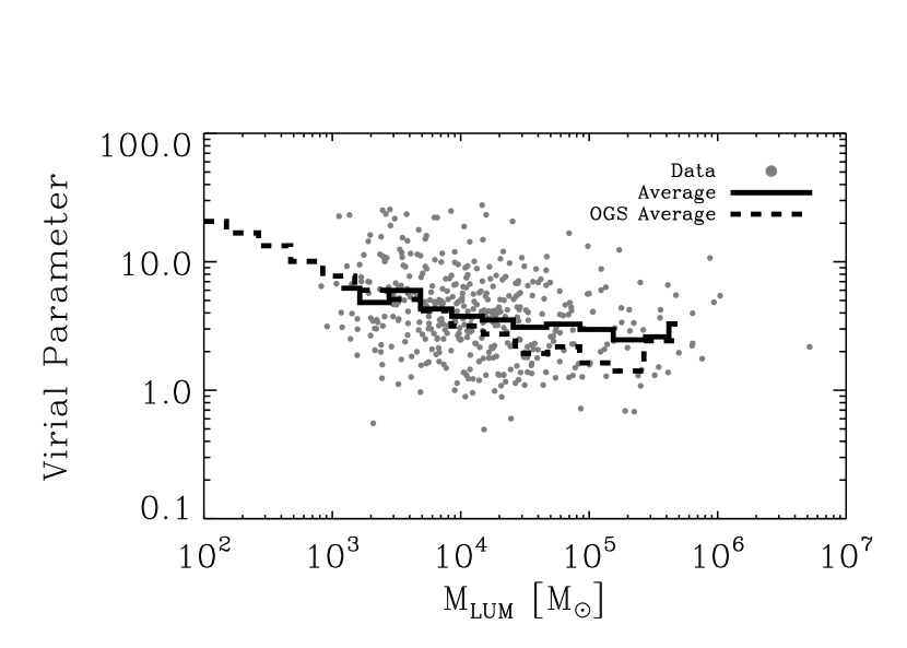
Figure 2.— Virial Parameter as a Function of Luminous Mass for Clouds in the Perseus Arm. Gray dots indicate the 431 clouds for which the virial and luminous mass can both be determined. The solid black line is the average of the data in bins of 0.25 dex in mass. For comparison, the average virial parameter is plotted as a function of mass for the clouds in the OGS catalog (dashed line). The two data sets show similar virial parameters at all masses, recovering nearly the same virial parameter for a given mass.

6.3. Conclusions

We have presented a method for measuring macroscopic GMC properties — spatial size, line width, and luminosity — from a region of emission in a spectral line data cube. This method corrects for biases from limited sensitivity and resolution and produces reliable results that are directly comparable among a wide variety of data sets. We correct for limited sensitivity via an extrapolation to a theoretical 0 Kelvin isosurface. We apply a simple quadratic deconvolution to the extrapolated values to account for resolution biases. We find that bootstrapping methods yield believable estimates of the uncertainties in the derived parameters. We present a set of suggestions for transforming the derived properties into physical quantities of interest. In the Appendix to this paper we present a new method for decomposing emission into individual GMCs. This method is conservative and robust, designed to produce robust results from low resolution/sensitivity data. In this section we have applied all of these methods to an array of extragalactic (Local Group) and Galactic data. We find that the algorithm reproduces established results for Galactic GMCs and that the sensitivity and resolution biases are potentially significant — often $\sim 40\%$ — for even the most recent Local Group GMC measurements.

Based on this investigation of the observational biases in measuring molecular cloud properties, we note several important points that should be considered in planning observations of GMCs and interpreting the results. First, resolution and sensitivity biases can be corrected to $<10\%$ error provided the cloud has a modest peak signal-to-noise ($T_{peak}/\sigma_{RMS}\gtrsim 10$) and is marginally resolved $R_{cld}>0.8\theta_{\mathrm{FWHM}}$, where $\theta_{\mathrm{FWHM}}$ is the full width at half maximum extent of the beam. Given current and future telescope capabilities, even the properties of extragalactic GMCs can be accurately measured. From Figure 1, we can see that single dish surveys can accurately study clouds more massive than $10^{4}~{}M_{\odot}$ in the Magellanic clouds and careful interferometer observations can recover cloud properties for clouds with mass $M\gtrsim 10^{5}~{}M_{\odot}$ in M31 and M33. However, interferometer observations systematically underestimate molecular cloud properties. All else being equal, interferometers can underestimate fluxes by 40% and cloud radii by 10% relative to single-dish observations. Line widths are largely unaffected by interferometer observations. The magnitude of the systematic bias depends on the array configuration and the sensitivity of the observations. In general, wider coverage of the $(u,v)$ plane produces better property recovery. To minimize bias, observers should favor observations from several array configurations or from arrays with many elements. If possible, the interferometer data should be supplemented with single-dish observations. Finally, the decomposition algorithm used to separate emission into physically relevant structures will systematically affect molecular cloud properties. To date, there is no algorithm that should be favored in all circumstances, but any comparative study of GMC properties should be consistent in the choice of algorithm. For example, the results of a CLUMPFIND algorithm applied to an extragalactic data set are not directly comparable to a catalog produced by a simple contouring method applied to Milky Way data. Provided the same algorithm is used across multiple data sets, referencing algorithm parameters to a common physical scale will minimize systematic differences.

We will make a software version of the decomposition and measurement algorithm available as an IDL package. Further, since methodology can affect the results of GMC studies so strongly, we encourage authors working in the field to make their data available to the community after publication in order to facilitate future rigorous comparisons.

Appendix A Appendix: A New Decomposition Algorithm

The choice of what emission to identify as a GMC may be the single largest source of uncertainty in measuring and comparing GMC properties. A number of methods have been employed over the years, from simple contouring methods (e.g.  Sanders et al., 1985; Dame et al., 1986; Solomon et al., 1987; Heyer et al., 2001) to fitting three-dimensional Gaussians (GAUSSCLUMPS, Stutzki & Güsten, 1990; Kramer et al., 1998), to modified watershed algorithms (CLUMPFIND and its kin, Williams et al., 1994; Brunt et al., 2003).

In this section we present a new decomposition algorithm that is designed to identify clouds at low sensitivities while avoiding the introduction of a false clouds due to noise. This algorithm consists of two parts: identifying regions of significant emission in the data set and then assigning this emission to individual “clouds.”

A.1. Signal Identification

We first identify regions of contiguous, significant emission in our position-position-velocity data cube. We estimate the noise in the data set by measuring the RMS intensity, $\sigma_{RMS}$, from a signal-free region of the data cube. We then construct a high-significance mask. This mask includes only adjacent channels that both have intensities above $4\sigma_{RMS}$. We expand that mask to include all emission above a lower threshold — typically two channels above $2\sigma_{RMS}$ significance — that is connected to the original high significance mask through pixels with $\geq 2\sigma_{RMS}$ significance. The resulting mask contains most of the significant emission in the data cube. Lowering the threshold below two channels at $\approx 1.5\sigma_{RMS}$ runs the risk of biasing the moment measurements towards high values by including false emission (noise with positive values) in the cloud.

A.2. Cloud Identification

In this section, we describe the algorithm used to decompose a region of emission into individual subsections representing the physically distinct entities in the data (“clouds”). Through the description of the algorithm, there are several parameters that can be varied to produce changes in the resulting decomposition. In general, we set these parameters using physical prior knowledge of the GMCs we are seeking to catalog. We discuss the choice of these parameters in the following section.

1. Discard Small or Low Contrast Regions: If a region is too small for us to measure meaningful properties from it, we discard the region. We require that each region has an area larger than two beam sizes, so that we can measure its size; and a velocity width of more than a single channel, so that we can measure its line width. If the intensity contrast between the peak and the edge of the region is less than a factor of two, we lack the dynamic range needed to correct the sensitivity bias and we therefore discard the region. If a region is not discarded we proceed to the next step.

2. Rescale the Data to Reduce the Effects of Substructure: Molecular clouds contain significant substructure that confuses the decomposition of these sources. The substructure is often significantly brighter than bulk of the gas in the cloud. We rescale the data to reduce the contrast between this substructure and the cloud as a whole. The data are rescaled using the following transform:

   $$T^{\prime}=\left\{\begin{array}[]{cl}T&;~{}T<T_{clip},\\ T_{clip}[1+{\arctan(T/T_{clip}-1)}]&;~{}T\geq T_{clip}.\\ \end{array}\right.$$

   This transform reduces the contrast pixels with $T\gtrsim 2T_{clip}$ while preserving the relative brightness distribution. The value of $T_{clip}$ is left as a free parameter. The transformed data are used in the decomposition algorithm. Such brightness transforms are frequently used in the decomposition algorithms used in other fields such as medical imaging (e.g.  Lin et al., 2003).

3. Identify Independent Local Maxima: We identify potential local maxima, by identifying the elements in the data cube that are larger than all their neighbors. We consider neighbors to be all data that lie within a box with side length $D_{max}$ in position and $\Delta V_{max}$ in velocity centered on the local maximum. These are our “candidate maxima.” The parameters $D_{max}$ and $\Delta V_{max}$ are free parameters. If we find more than one candidate maximum in a region of emission, we proceed to the next steps to further verify each maximum’s independence. If we find a single candidate maximum then we label the region as a cloud and measure its properties as described in the main paper.

4. Find Shared Isosurfaces and Reject Small Clouds or those with Smooth Mergers: For each pair of candidate maxima we calculate the value of the highest intensity isosurface to contain both maxima. We refer to this highest shared isosurface as the merge level. Using this set of highest shared isosurfaces, we calculate three properties of interest:

   1. The area uniquely associated with each maximum (i.e. the area above the merge level for that maximum).

   2. The antenna temperature interval between the merge level and each maximum, referred to as the contrast interval.

   3. The fractional amount by which each of the (unextrapolated) moment values changes across each shared isosurface (i.e. $\frac{\Delta\sigma_{maj}}{\sigma_{maj}}$ for each maximum across each shared isosurface). We consider the two clouds to merge smoothly across the isosurface only if:

      1. None of the second moments increase by more than 100% for both maxima.

      2. No two of the second moments increase by more than 50% for both maxima.

      3. The flux increases by less 200% for both maxima.

   We use these three properties to pare maxima from the region. We reject maxima associated with small areas (less than two beam sizes, as for the region above) and contrast intervals less than $\Delta T_{max}$, a free parameter. Choosing $\Delta T_{max}\geq 2\sigma$ significantly reduces the effects of noise on decomposition (e.g.  Brunt et al., 2003) since noise is associated with low contrast intervals. Finally, when a pair of maxima merge smoothly across a shared isosurface, we keep the higher intensity maximum and discard the lower one. This is a conservative choice in the decomposition algorithm: unless merging the two kernels significantly alters the properties of one of the clouds associated with the separate kernels, we assume the kernels are not physically distinct. The effect of removing kernels that merge smoothly from our data set is to reduce the algorithm’s sensitivity to substructure within clouds. We iterate this step until we have a set of maxima associated with the required areas and separated from each other by significant jumps in their properties.

5. Define Clouds Using Shared Isosurfaces: The surviving maxima each correspond to a “cloud.” That cloud consists of the emission within the lowest intensity isosurface uniquely associated with the cloud. Emission that lies below this isosurface is part of a “watershed” shared among clouds and we do not assign it to any cloud. By not considering contested emission, i.e. emission that could be associated with distinct local maxima, we avoid the problem of how to properly assign this emission to local maxima.

6. Measure Cloud Properties: Finally, we apply the methods described in §2 and 3 to derive spatial sizes, line widths, and luminosities for each cloud. The transformed data (Step 2) are inverse transformed into the original brightness units for this analysis.

A.3. Using Physical Priors to Establish Algorithm Parameters

Several of the algorithm’s parameters are left to the choice of the user. Without any prior knowledge of the physical objects in the data, we establish default values for these parameters that will produce a reasonable decomposition based solely on the characteristics of the data. These defaults are chosen to provide sensitivity to real substructure within the data without contamination by noise and can be regarded as the minimum appropriate values for these parameters in most cases. The free parameters in the algorithm are the brightness transform threshold ($T_{clip}$, Step 2) position and velocity window size used in searching for local maxima ($D_{max}$ and $\Delta V_{max}$, Step 3), and the minimum contrast temperature ($\Delta T_{max}$, Step 4b). Without prior knowledge of substructure in the data, no brightness transform should be applied ($T_{clip}=\infty$). The minimum values for the parameters in the search for initial local maxima are set by the resolution of the data: $D_{max}=\theta_{beam}$ and $\Delta V_{max}=\Delta V_{chan}$ or else separations between local maxima cannot be resolved. Finally, we use $\Delta T_{max}=2\sigma_{RMS}$ to prevent the noise in the data set from being recognized by the algorithm as legitimate structure and becoming the basis for the decomposition.

In the main section of the paper, we developed methods that measured physical properties of molecular emission without observational bias. Ideally, the decomposition algorithm used in the analysis would also be free of observational bias. A good algorithm would, for example, decompose the same emission into similar structures regardless of the resolution and sensitivity of the observations. To progress towards this goal, we set the parameters of the decomposition algorithm to have similar values in physical units (pc, km s^-1, K) rather than data units (beam widths, channels, $\sigma_{RMS}$).

In the molecular ISM, which has structure on a range of scales, the choice of the physical values for the algorithm parameters must be motivated by prior knowledge of the objects that we wish to identify. The choice of parameters for identifying GMCs would be different from the choice of parameters for identifying clumps and cores. As a population, GMCs have size scales of 10s of parsecs, line widths of several km s^-1, and brightness temperatures of $T\lesssim 10$ K (e.g.  Solomon et al., 1987). In contrast, the clumpy substructure within clouds has a size scale of 1 pc, line widths of order 1 km s^-1 and can have brightness temperatures of 30 K or higher (e.g.  Williams et al., 1994). We select the parameters of the algorithm to find molecular clouds rather than the clumps within them. In particular, we set the minimum separation between local maxima as $D_{max}=15$ pc and the velocity separation to be $\Delta V_{max}=2$ km s^-1. We also fix a contrast interval in antenna temperature of $\Delta T_{max}=1$ K rather than the data-driven value of $2\sigma_{RMS}$. Finally, we must account for the presence of bright molecular gas substructure within molecular clouds. For example, Orion A has a few distinct regions separated by $>15$ pc with antenna temperatures in excess of 15 K (Wilson et al., 2005). These are associated with hot molecular gas around young stars like the Trapezium cluster. In general, the typical kinetic temperature of gas in GMCs is $\sim 10$ K so brightness temperatures in excess of 10 K are usually associated with structure within molecular clouds not changes from cloud to cloud. Hence, to catalog clouds and not substructure, we must reduce the influence of the high $T_{b}$ data with the parameter $T_{clip}$. We use $T_{clip}=2.5$ K to maintain the full sensitivity for the gas separating GMCs (which typically has $T_{A}\lesssim 5$ K in the Solomon et al. (1987) data) while reducing the influence of brighter gas associated with a single GMC. Using $T_{clip}=2.5$ K has little influence on extragalactic data where beam deconvolution typically averages out the presence of bright substructure within the clouds.

We summarize our choices of parameters in Table 2 when the parameters are motivated by the data (Data-Based) or by physical assumptions about the structures being extracted (GMC Physical Priors). The resolution or the sensitivity of a data set may be sufficiently poor that the physical parameters are unattainable in the data set (e.g. $\theta_{beam}>15~{}$pc, $2\sigma_{rms}>1$ K). In this case, the decomposition must be regarded with caution as it may not be directly comparable to other data sets. The adopted values are appropriate for decomposing data sets of ¹²CO emission. The values of $T_{clip}$ and $\Delta T_{max}$ would be different for other tracers.

Table 2Parameter Choices for Decomposition Algorithm

Parameter	Data-Based	GMC Physical Priors
$T_{clip}$	$\infty$	2.5 K
$D_{max}$	1 beam width	15 pc
$\Delta V_{max}$	1 channel	2 km s-1
$\Delta T_{max}$	$2\sigma_{RMS}$	1 K

A.4. Comparison with Existing Algorithms

To demonstrate that the proposed algorithm is actually an improvement on existing methods, we analyze trial data sets with known properties using this algorithm and compare the results to those from the GAUSSCLUMPS and CLUMPFIND algorithms to the trial data. We use the CLFIND algorithm implemented in MIRIAD (Sault et al., 1995) and our own IDL implementation of the Kramer et al. (1998) GAUSSCLUMPS algorithm, which we have compared to the standard algorithm operating on a real data set with satisfactory results.

We first examine how adept the three algorithms are at decomposing a pair of blended clouds. We construct a series of data cubes with two unresolved model clouds separated in position by a variable distance. The model clouds each have a peak signal-to-noise ratio of 10 with a Gaussian line profile. For each value of the separation, we decompose 100 data cubes with different realizations of the noise using the three algorithms, using data based choices for the algorithm parameters. Figure A.4 (left) shows the mean number of clouds recovered by each algorithm as a function of the separation (we count clouds with peak signal-to-noise larger than 5 as “recovered”). As the trial clouds are moved farther apart, the typical number of clouds detected by each algorithm increases by 1. However, only the algorithm presented here consistently recovers a single cloud at low separations. GAUSSCLUMPS and CLUMPFIND produce false clouds from the noise. The jump in the number of clouds detected by the GAUSSCLUMPS algorithm occurs where the separation equals the resolution, whereas both the current algorithm and CLUMPFIND are able to distinguish the clouds only if their separation is over 1.5 times the resolution. GAUSSCLUMPS appears to be able to distinguish tight blends of clouds but is the most susceptible to noise.

The mean number of clouds with $T_{peak}/\sigma_{RMS}>5$ recovered by three different decomposition algorithms on trial data. (left) The three algorithms applied to a blend of two Gaussian clouds. The results of using algorithm from the present study are minimally affected by the presence of noise. (right) The three algorithms applied to a circular top-hat cloud showing the effects of non-Gaussian shape on the results of the algorithms. The current algorithm is the best for grouping together large structures with non-Gaussian shapes.

As a second test of the algorithms, we compared the number of clouds that the algorithms recover from a single cloud with a circular top-hat brightness profile ($T_{A}=\mbox{const. for }r<R_{0};~{}0$ otherwise) and peak signal-to-noise of 10. The size of the cloud is varied with respect to the resolution of the data set and 100 data sets for each value of $R_{0}$ are decomposed by each algorithm. The non-Gaussian brightness profile confounds all of the algorithms but to varying degrees. CLUMPFIND detects an increasing number of spurious clouds as the cloud grows, suggesting that the number of false clouds grows with the volume studied. Despite the non-Gaussian profile, GAUSSCLUMPS does surprisingly well with large sources. The current algorithm, however, does the best job of detecting a single source in the presence of noise. For analyzing data with a relatively low signal-to-noise, we find the decomposition algorithm presented in this Appendix should be favored for identifying clouds.

A.5. Applying the Algorithm to the Orion-Monoceros Region

The Orion Molecular Cloud is among the best studied of all GMCs, so it is an good place to compare the results of our methods to those of previous work. For this comparison, we use the data and results of the recent, uniform survey of the entire Orion-Monoceros region by Wilson et al. (2005). We analyze their final data set using the methods in this paper (with physical priors for the decomposition algorithm parameters) and summarize the results in Figure A.5, an integrated intensity map of the region. The decomposition results in 81 molecular clouds, most of which are associated with the Galactic plane at the top of the Figure.

Masked, integrated-intensity map of the Orion-Monoceros region with a logarithmic stretch. The ellipses plotted over the data indicate the positions, sizes and orientations of molecular clouds identified by our decomposition algorithm. In general, the algorithm does a good job of identifying known molecular clouds as single entities. Notable molecular features are labeled.

The results of the algorithms decomposition of the region are good: major molecular clouds are identified as single entities in the decomposition. The algorithm succeeds where other cloud identification schemes would face difficulty. Nearly all of the emission in the data is connected above a single isosurface so that simple contouring methods would identify the entire Orion-Monoceros region as a single molecular cloud, though more complicated algorithms (Scoville et al., 1987) may succeed. CLUMPFIND and GAUSSCLUMPS would isolate individual peaks and decompose clouds into their substructure — as was intended by their design (CLUMPFIND identifies 617 clumps in the same data).

The properties of the clouds agree well with the values published for a human decomposition of the emission. The results of the analysis are given in Table 3. For comparison, we adopt the distances of Wilson et al. (2005). We compare the results of the algorithm to their results, after scaling their mass up by 10% to account for a difference in the adopted CO-to-H₂ conversion factors. In several cases the masses agree quite well (to within 5%, Orion A, Mon R2, Scissors), while other features show $\sim 30\%$ differences. These systematic discrepancies arise from differences in how emission is assigned into structures. For example, the algorithm only identifies the central region of Orion B as a molecular cloud; it does not include emission near the location of Orion East that is nominally part of the Orion B cloud because the assignment of this emission is contested with neighboring clouds. Similarly, the algorithm characterizes the Northern Filament region as five distinct clouds rather than the single large cloud that a human decomposition produced. Despite these differences, the results of the algorithm are reassuring – in most cases, the well-known molecular clouds are identified as single clouds and there is good agreement between their derived physical properties and the results of previous studies.

Table 3 Properties of Major Molecular Clouds in Orion-Monoceros

Name	Distance	$M_{\mathrm{human}}$	$M_{\mathrm{algorithm}}$	$R_{e}$	$\sigma_{v}$	$\alpha$
	(pc)	($10^{4}M_{\odot}$)	($10^{4}M_{\odot}$)	(pc)	(km s-1)
Orion A	480	12.	$11.\pm 0.06$	$18.6\pm 0.2$	$2.9\pm 0.1$	$1.6\pm 0.1$
Orion B	500	9.1	$5.6\pm 0.08$	$12.1\pm 0.3$	$1.5\pm 0.1$	$0.6\pm 0.1$
Orion East	120	0.013	$0.013\pm 0.001$	$1.2\pm 0.1$	$\cdots$	$\cdots$
Mon R2	800	12.	$11.\pm 0.5$	$25.9\pm 1.2$	$1.6\pm 0.1$	$0.7\pm 0.1$
Crossbones	470	1.9	$0.57\pm 0.02$	$11.0\pm 0.6$	$0.8\pm 0.1$	$1.5\pm 0.3$
Northern Filament	390	1.9	$1.2\pm 0.07$	$8.6\pm 0.7$	$1.7\pm 0.1$	$2.6\pm 0.5$

A.6. Decomposing Orion-like Clouds in Other Galaxies

As a final test of the decomposition and analysis algorithm, we apply the algorithm to simulated observations of the Orion-Monoceros region with beam sizes and signal-to-noise values typical of extragalactic GMC observations. We simulate observations by convolving the data set to the desired resolution and adding a convolved data cube of noise which is scaled up to give the desired peak signal-to-noise ratio in the data. We perform this for a peak signal-to-noise ($S/N$) values of 10 and 30 combined with beam sizes of 10, 20 and 50 pc. The results of the decompositions are displayed in Figure A.6.

At coarse resolution and low sensitivity, the fainter clouds are undetectable. However, the algorithm identifies each of Orion A, Orion B, Mon R2 and the Northern Filament in at least one of the trial data sets. At high resolution (10 pc) and peak signal-to-noise ($S/N=30$), the algorithm successfully identifies the clouds with properties that are consistent, within the uncertainties determined by the algorithm, with the masses of the clouds in Table 3. The systematic effects of poor resolution manifest themselves for beam sizes $\gtrsim 20$ pc where the decomposition of blended emission results in $\sim 20\%$ variations in the properties of the clouds relative to those found in the original data set for both high and low $S/N$. For a beam size of 20 pc, the clouds are not resolved since this is over twice the size of the clouds along their minor axes. Finally, at 50 pc resolution, Mon R2 is not found by the algorithm and high $S/N$ is required to distinguish Orion A and Orion B. There is a variation of 100% (0.3 dex) in the derived physical parameters for the clouds; this variation is reflected in the estimates of the uncertainties. As expected based on the 20 pc resolution data, the clouds are not spatially resolved for a beam size of 50 pc. An accurate decomposition of emission into typical Galactic GMCs requires a beam size $\sim 20$ pc though only a modest sensitivity is required: $S/N\gtrsim 10$.

The Orion-Monoceros Region convolved to the typical signal-to-noise ($S/N$) and spatial resolution (beam size) of extragalactic observations. The integrated intensity map of the cloud is drawn as a contour plot with the positions and sizes of clouds that the algorithm identifies drawn as gray ellipses. Contours on the integrated intensity map are drawn at -0.1 (dashed), 0 (bold), 0.1, 0.2, … 1.0 times the peak value in the map. The sizes of the clouds are not deconvolved from the beam, so coarser spatial resolution results in objects that are apparently larger. Except in the marginally resolved, low $S/N$ case, the algorithm successfully identifies Orion A and B. Mon R2 and the Northern Filament appear in maps with higher resolution and signal-to-noise.

References

- Bertoldi & McKee (1992) Bertoldi, F., & McKee, C. F. 1992, ApJ, 395, 140
- Blitz (1985) Blitz, L. 1985, ApJ, 296, 481
- Blitz & Stark (1986) Blitz, L. & Stark, A. A. 1986, ApJ, 300, L89
- Blitz & Thaddeus (1980) Blitz, L., & Thaddeus, P. 1980, ApJ, 241, 676
- Bolatto et al. (2003) Bolatto, A. D., Leroy, A., Israel, F. P., & Jackson, J. M. 2003, ApJ, 595, 167
- Brunt et al. (2003) Brunt, C. M., Kerton, C. R., & Pomerleau, C. 2003, ApJS, 144, 47
- Dame et al. (1986) Dame, T. M., Elmegreen, B. G., Cohen, R. S., & Thaddeus, P. 1986, ApJ, 305, 892
- Dame et al. (2001) Dame, T. M., Hartmann, D., & Thaddeus, P. 2001, ApJ, 547, 792
- Fukui et al. (1999) Fukui, Y., et al. 1999, PASJ, 51, 745
- Helfer et al. (2002) Helfer, T. T., Vogel, S. N., Lugten, J. B., & Teuben, P. J. 2002, PASP, 114, 350
- Heyer et al. (1998) Heyer, M. H., Brunt, C., Snell, R. L., Howe, J. E., Schloerb, F. P., & Carpenter, J. M. 1998, ApJS, 115, 241
- Heyer et al. (2001) Heyer, M. H., Carpenter, J. M., & Snell, R. L. 2001, ApJ, 551, 852
- Israel et al. (1993) Israel, F. P., et al. 1993, A&A, 276, 25
- Koda et al. (2005) Koda, J., Sawada, T., Hasegawa, T., & Scoville, N. 2005, ApJ, in press.
- Kramer et al. (1998) Kramer, C., Stutzki, J., Rohrig, R., & Corneliussen, U. 1998, A&A, 329, 249
- Leroy et al. (2005) Leroy, A., Bolatto, A., Walter, F., & Blitz, L. 2005, in preparation
- Lin et al. (2003) Lin, G., Adiga, U., Olson, K., Guzowski, J., Barnes, C., & Roysam, B. 2003, Cytometry A, 56, 23
- McKee & Zweibel (1992) McKee, C. F. & Zweibel, E. G. 1992, ApJ, 399, 551
- Polk et al. (1988) Polk, K. S., Knapp, G. R., Stark, A. A., & Wilson, R. W. 1988, ApJ, 332, 432
- Rosolowsky et al. (2003) Rosolowsky, E., Engargiola, G., Plambeck, R., & Blitz, L. 2003, ApJ, 599, 258
- Rosolowsky (2005) Rosolowsky, E., ApJ, submitted.
- Sanders et al. (1985) Sanders, D. B., Scoville, N. Z., & Solomon, P. M. 1985, ApJ, 289, 373
- Sanders et al. (1986) Sanders, D. B., Clemens, D. P., Scoville, N. Z., & Solomon, P. M. 1986, ApJS, 60, 1
- Sault et al. (1995) Sault, R. J., Teuben, P. J., & Wright, M. C. H. 1995, in ASP Conf. Ser. 77: Astronomical Data Analysis Software and Systems IV, 433–+
- Sheth et al. (2000) Sheth, K., Vogel, S. N., Wilson, C. D., & Dame, T. M. 2000, Proceedings 232. WE-Heraeus Seminar, 37
- Solomon et al. (1987) Solomon, P. M., Rivolo, A. R., Barrett, J., & Yahil, A. 1987, ApJ, 319, 730
- Stutzki & Güsten (1990) Stutzki, J. & Güsten, R. 1990, ApJ, 356, 513
- Scoville et al. (1987) Scoville, N. Z., Yun, M. S., Sanders, D. B., Clemens, D. P., & Waller, W. H. 1987, ApJS, 63, 821
- Taylor et al. (1999) Taylor, C. L., Hüttemeister, S., Klein, U., & Greve, A. 1999, A&A, 349, 424
- Thompson et al. (2001) Thompson, A. R., Moran, J. M., & Swenson, G. W. 2001, Interferometry and synthesis in radio astronomy by A. Richard Thompson, James M. Moran, and George W. Swenson, Jr. 2nd ed. New York : Wiley, c2001.xxiii, 692 p. : ill. ; 25 cm. ”A Wiley-Interscience publication.” Includes bibliographical references and indexes. ISBN : 0471254924,
- Vogel et al. (1987) Vogel, S. N., Boulanger, F., & Ball, R. 1987, ApJ, 321, L145
- Walter (2005) Walter, F. 2005, in preparation
- Williams et al. (1994) Williams, J. P., de Geus, E. J., & Blitz, L. 1994, ApJ, 428, 693
- Wilson et al. (2005) Wilson, B. A., Dame, T. M., Masheder, M. R. W., & Thaddeus, P. 2005, A&A, 430, 523
- Wilson & Scoville (1990) Wilson, C. D. & Scoville, N. 1990, ApJ, 363, 435
- Wilson & Reid (1991) Wilson, C. D., & Reid, I. N. 1991, ApJ, 366, L11
- Wilson & Rudolph (1993) Wilson, C. D., & Rudolph, A. L. 1993, ApJ, 406, 477
- Wright (1996) Wright, M. C. H. 1998, BIMA Memorandum Series, 69