SCREW INSTABILITY OF MAGNETIC FIELD AND GAMMA-RAY BURSTS IN TYPE IB/C SUPERNOVAE

Abstract

A toy model for gamma-ray burst supernovae (GRB-SNe) is discussed by considering the effects of screw instability of magnetic field in black hole (BH) magnetosphere. The screw instability in the Blandford-Znajek (BZ) process (henceforth SIBZ) can coexist with the screw instability in the magnetic coupling (MC) process (henceforth SIMC). It turns out that both SIBZ and SIMC occur inevitably, provided that the following parameters are greater than some critical values, i.e., (i) the BH spin, (ii) the power-law index describing the magnetic field at the disk, and (iii) the vertical height of the astrophysical load above the equatorial plane of the rotating BH. The features of several GRBs are well fitted. In our model the durations of the long GRBs depend on the evolve time of the half-opening angle. A small fraction of energy is extracted from the BH via the BZ process to power a GRB, while a large fraction of energy is extracted from the BH via the MC process to power an associated supernova. In addition, the variability time scales of tens of msec in the light curves of the GRBs are fitted by two successive flares due to SIBZ.

1 INTRODUCTION

Recently, observations and theoretical considerations have linked long-duration GRBs with ultra-bright Type Ib/c supernovae (SNe; Galama et al. 1998, 2000; Bloom et al. 1999). The first candidate was provided by SN 1998bw and GRB 980425, and the recent HETE-II burst GRB 030329 has greatly enhanced the confidence in this association (Stanek et al. 2003; Hjorth et al. 2003). Extremely high energy released in very short time scale suggests that GRBs involve the formation of a black hole (BH) via a catastrophic stellar collapse event or possibly a neutron star merger, implying that an inner engine could be built on an accreting BH.

Among a variety of mechanisms of powering GRBs the Blandford-Znajek (BZ) process (Blandford & Znajek, 1977) has its unique advantage in providing “clean” (free of baryonic contamination) energy by extracting rotating energy from a BH and transferring it in the form of Poynting flow in the outgoing energy flux (Lee et al. 2000, hereafter Lee00; Li 2000c, hereafter Li00).

Not long ago Brown et al. (2000, hereafter B00) worked out a specific scenario for a GRB-SN connection. They argued that the GRB is powered by the BZ process, and the SN is powered by the magnetic coupling (MC) process, which is regarded as one of the variants of the BZ process (Blandford 1999; van Putten 1999; Li 2000b, 2002; Wang, Xiao & Lei 2002, hereafter W02). It is shown in B00 that about $10^{53}ergs$ are available to power both a GRB and a SN. However, they failed to distinguish the fractions of the energy for these two objects.

More recently, van Putten and his collaborators (van Putten 2001; van Putten & Levinson 2003, hereafter P03) worked out a poloidal topology for the open and closed magnetic field lines, in which the separatrix on the horizon is defined by a finite half-opening angle. The duration of a GRB is set by the lifetime of the rapid spin of the BH. It is found that GRBs and SNe are powered by a small fraction of the BH spin energy. This result is consistent with observations, i.e., duration of GRBs of tens of seconds, true GRB energies distributed around $5\times 10^{50}ergs$ (Frail et al. 2001), and aspherical SNe kinetic energies of $2\times 10^{51}ergs$ (Hoflich et al. 1999).

Very recently, Lei et al. (2005, hereafter Lei05) proposed a scenario for GRBs in type Ib/c SNe invoking the coexistence of the BZ and MC processes. In Lei05 the GRB is powered by the BZ process, and the associated SN is powered by the MC process. The overall time scale of the GRB is fitted by the duration of the open magnetic flux on the horizon.

Besides the features of high energy released in very short durations most GRBs are highly variable, showing very rapid variations in flux on a time scale much shorter than the overall duration of the burst. Variability on a time scale of milliseconds has been observed in some long bursts (Norris et al. 1996; McBreen et al., 2001; Nakar and Piran, 2002). Unfortunately, the origin of the variations in the fluxes of GRBs remains unclear. In this paper we intend to discuss the mechanism for producing the variations in the fluxes of GRBs by virtue of the screw instability in BH magnetosphere.

It is well known that the magnetic field configurations with both poloidal and toroidal components can be screw-unstable. According to the Kruskal-Shafranov criterion the screw instability will occur, if the toroidal magnetic field becomes so strong that the magnetic field line turns around itself once or more (Kadomtsev 1966; Bateman 1978).

Some authors have addressed the screw instabilities in BH magnetosphere. Gruzinov (1999) argued that the magnetic field with a bunch of closed field lines connecting a Kerr BH with a disk can be screw-unstable, resulting in the release of magnetic energy with the flares at the disk. Li (2000a) discussed the screw instability of the magnetic field in the BZ process, leading to a stringent upper bound to the BZ power. Wang et al. (2004, hereafter W04) studied the screw instability in the MC process. They concluded that this instability could occur at some place away from the inner edge of the disk, provided that the BH spin $a_{*}$ and the power-law index $n$ for the variation of the magnetic field on the disk are greater than some critical values.

In this paper we attempt to combine the screw instability of the magnetic field with the coexistence of the BZ and MC processes. To facilitate the description henceforth we refer to the screw instability of the magnetic field occurring in the BZ and MC processes as SIBZ and SIMC, respectively. It is shown that both SIBZ and SIMC can occur, provided that the following parameters are greater than some critical values: (1) the BH spin, (2) the power-law index describing the variation of the magnetic field at the disk, and (3) the vertical height of the astrophysical load above the equatorial plane of the Kerr BH.

The features of several GRB-SNe are well fitted in our model. (1) The overall duration of the GRBs is fitted by the evolution of the half-opening angles. (2) The true energies of several GRBs are fitted by the energy extracted in the BZ process, and the energies of associated SNe are fitted by the energy transferred in the MC process. (3) The variability time scales of tens of msec in the light curves of several GRBs are fitted by two successive flares due to SIBZ.

This paper is organized as follows. In $\S$ 2 we derived a criterion of SIBZ based on the Kruskal-Shafranov criterion and some simplified assumptions on the remote load. In $\S$ 3 we discuss the time scale and energy extraction from a Kerr BH in the context of the suspended accretion state. In $\S$ 4 we propose a scenario for the origin of the variation in the light curves of GRBs based on the flares arising from SIBZ. Finally, in $\S$ 5, we summarize the main results and discuss some issues related to our model. Throughout this paper the geometric units $G=c=1$ are used.

2 SCREW INSTABILITY IN BH MAGNETOSPHERE

In W04 the criterion of SIMC is derived based on the following points: (1) the Kruskal-Shafranov criterion, (2) the mapping relation between the angular coordinate on the BH horizon and the radial coordinate on the disk, and (3) the calculations of the poloidal and toroidal components of the magnetic field at the disk. The criterion of SIBZ can be derived in an analogous way. However, the BZ process involves unknown astrophysical loads, to which both the mapping relation and the calculations for the poloidal and toroidal components of the magnetic field are related. In order to work out an analytical model we present some simplified assumptions as follows.

(1) The magnetosphere anchored in a Kerr BH and its surrounding disk is described in Boyer-Lindquist coordinates, in which the following Kerr metric parameters are involved (MacDonald and Thorne 1982, hereafter MT82).

$$\left\{{\begin{array}[]{l}\Sigma^{2}=\left({r^{2}+a^{2}}\right)^{2}-a^{2}\Delta\sin^{2}\theta,\mbox{ }\rho^{2}=r^{2}+a^{2}\cos^{2}\theta,\mbox{ }\\ \Delta=r^{2}+a^{2}-2Mr,\mbox{ }\varpi=\left({\Sigma\mathord{\left/{\vphantom{\Sigma\rho}}\right.\kern-1.2pt}\rho}\right)\sin\theta,\\ \alpha={\rho\sqrt{\Delta}}\mathord{\left/{\vphantom{{\rho\sqrt{\Delta}}\Sigma}}\right.\kern-1.2pt}\Sigma.\\ \end{array}}\right.$$ (1)

(2) The remote load is axisymmetric, being located evenly in a plane with some height above the disk. In Figure 1 the open magnetic field lines connect the BH horizon with the load. The symbol $L_{BZ}$ and $H_{c}$ represent the critical field line and the height of the remote load above the equatorial plane for the occurrence of SIBZ, respectively.

(3) In Figure 1 the radius $r_{{}_{S}}$ is the critical radius of SIMC, which is determined by the criterion of the screw instability given in W04,

$${\left({{2\pi\varpi_{{}_{D}}}\mathord{\left/{\vphantom{{2\pi\varpi_{{}_{D}}}{L_{MC}}}}\right.\kern-1.2pt}{L_{MC}}}\right)B_{D}^{p}}\mathord{\left/{\vphantom{{\left({{2\pi\varpi_{{}_{D}}}\mathord{\left/{\vphantom{{2\pi\varpi_{{}_{D}}}{L_{MC}}}}\right.\kern-1.2pt}{L_{MC}}}\right)B_{D}^{p}}{B_{D}^{T}}}}\right.\kern-1.2pt}{B_{D}^{T}}<1.$$ (2)

In equation (2) $L_{MC}$ is the critical length of the poloidal field line for SIMC, and $B_{D}^{p}$ and $B_{D}^{T}$ are the poloidal and toroidal components of the magnetic field on the disk, respectively, and $\varpi_{{}_{D}}$ is the cylindrical radius on the disk and it reads

$$\varpi_{{}_{D}}=\Sigma_{D}/\rho_{{}_{D}}=\xi M\chi_{ms}^{2}\sqrt{1+a_{*}^{2}\xi^{-2}\chi_{ms}^{-4}+2a_{*}^{2}\xi^{-3}\chi_{ms}^{-6}}.$$ (3)

where $\chi_{ms}\equiv\sqrt{{r_{ms}}\mathord{\left/{\vphantom{{r_{ms}}M}}\right.\kern-1.2pt}M}$ is defined by Novikov & Thorne (1973) in terms of the radius of innermost stable circular orbit (ISCO).

(4) The angle $\theta_{S}$ in Figure 1 is the half-opening angle of the magnetic flux tube on the horizon, which is related by the mapping relation between the angular coordinate on the BH horizon and the radial coordinate on the disk as follows (Wang et al., 2003, hereafter W03),

$$\cos\theta-\cos\theta_{L}=\int_{1}^{\xi}{\mbox{G}\left({a_{*};\xi,n}\right)d\xi},$$ (4)

where

$$\mbox{G}\left({a_{*};\xi,n}\right)=\frac{\xi^{1-n}\chi_{ms}^{2}\sqrt{1+a_{*}^{2}\chi_{ms}^{-4}\xi^{-2}+2a_{*}^{2}\chi_{ms}^{-6}\xi^{-3}}}{2\sqrt{\left({1+a_{*}^{2}\chi_{ms}^{-4}+2a_{*}^{2}\chi_{ms}^{-6}}\right)\left({1-2\chi_{ms}^{-2}\xi^{-1}+a_{*}^{2}\chi_{ms}^{-4}\xi^{-2}}\right)}}.$$ (5)

In equations (4) and (5) $\xi\equiv r\mathord{\left/{\vphantom{r{r_{ms}}}}\right.\kern-1.2pt}{r_{ms}}$ is defined as a radial parameter in terms of $r_{ms}$, and $n$ is a power-law index for the variation of the poloidal magnetic field at the disk, i.e.,

$$B_{D}^{p}\propto\xi^{-n}.$$ (6)

(5) The suspended accretion state is assumed due to the transfer of angular momentum from the BH to the disk (van Putten & Ostriker, 2001).

Analogous to equation (2) the criterion for SIBZ can be expressed as

$${\left({{2\pi R}\mathord{\left/{\vphantom{{2\pi R}{L_{BZ}}}}\right.\kern-1.2pt}{L_{BZ}}}\right)B_{L}^{p}}\mathord{\left/{\vphantom{{\left({{2\pi R}\mathord{\left/{\vphantom{{2\pi R}{L_{BZ}}}}\right.\kern-1.2pt}{L_{BZ}}}\right)B_{L}^{p}}{B_{L}^{T}}}}\right.\kern-1.2pt}{B_{L}^{T}}<1,$$ (7)

where $L_{BZ}$ is the critical length of the poloidal field line for SIBZ, and $B_{L}^{p}$ and $B_{L}^{T}$ are the poloidal and toroidal components of the magnetic field on the remote load, respectively, and $R$ is the cylindrical radius of the remote load with respect to the symmetric axis of the BH.

The toroidal field component $B_{L}^{T}$ can be expressed by Ampere’s law,

$$B_{L}^{T}={2I_{L}}\mathord{\left/{\vphantom{{2I_{L}}R}}\right.\kern-1.2pt}R,$$ (8)

where $I_{L}$ is the electric current flowing in the loop $KM{M}^{\prime}{K}^{\prime}$ in Figure 1 and it reads

$$I_{L}=\sqrt{{P_{BZ}}\mathord{\left/{\vphantom{{P_{BZ}}{Z_{L}}}}\right.\kern-1.2pt}{Z_{L}}}.$$ (9)

The quantities $P_{BZ}$ and $Z_{L}$ in equation (9) are the BZ power and the load resistance, respectively. The BZ power has been derived in W02 as follows,

$${P_{BZ}}\mathord{\left/{\vphantom{{P_{BZ}}{P_{0}}}}\right.\kern-1.2pt}{P_{0}}=2a_{*}^{2}\int_{0}^{\theta_{S}}{\frac{k\left({1-k}\right)\sin^{3}\theta d\theta}{2-\left({1-q}\right)\sin^{2}\theta}},$$ (10)

where $q\equiv\sqrt{1-a_{*}^{2}}$ is a parameter depending on the BH spin, and $k\equiv{\Omega_{F}}\mathord{\left/{\vphantom{{\Omega_{F}}{\Omega_{{}_{H}}}}}\right.\kern-1.2pt}{\Omega_{{}_{H}}}$ is the ratio of the angular velocity of the field lines to that of the BH horizon. The quantity $P_{0}$ is defined by

$$P_{0}\equiv\left({B_{H}^{p}}\right)^{2}M^{2}\approx 6.59\times 10^{50}\times B_{15}^{2}\left({M\mathord{\left/{\vphantom{M{M_{\odot}}}}\right.\kern-1.2pt}{M_{\odot}}}\right)^{2}erg\cdot s^{-1},$$ (11)

where $B_{15}$ represents the magnetic field at the BH horizon in terms of $10^{15}gauss$.

MT82 argued in a speculative way that the ratio $k$ will be regulated to about 0.5 by the BZ process itself, which corresponds to the optimal BZ power with the impedance matching. Taking the impedance matching into account, we have the remote load resistance equal to the horizon resistance, and they read

$$\Delta Z_{L}=\Delta Z_{H}=R_{H}\frac{\rho_{{}_{H}}d\theta}{2\pi\varpi_{{}_{H}}},$$ (12)

where $R_{H}=4\pi=377ohm$ is the surface resistivity of the BH horizon (MT82). Thus we have $Z_{L}$ and $Z_{H}$ expressed as

$$Z_{L}=Z_{H}=\int_{0}^{\theta_{S}}{R_{H}\frac{\rho_{{}_{H}}d\theta}{2\pi\varpi_{{}_{H}}}}=\int_{0}^{\theta_{S}}{\frac{2\rho_{{}_{H}}d\theta}{\varpi_{{}_{H}}}}$$ (13)

Incorporating equations (8)—(13), we can calculate $B_{L}^{T}$ in terms of the cylindrical radius $R$. On the other hand, the poloidal magnetic field $B_{L}^{P}$ at the radius $R$ of the load can be determined by the conservation of the magnetic flux, i.e.,

$$B_{H}^{P}2\pi\varpi_{{}_{H}}\rho_{{}_{H}}d\theta=B_{L}^{P}2\pi RdR.$$ (14)

From equation (14) we have

$$B_{L}^{P}=\frac{B_{H}^{P}\varpi_{{}_{H}}\rho_{{}_{H}}}{R}\frac{d\theta}{dR}.$$ (15)

Assuming that the height of the planar load above the equatorial plane of the Kerr BH is$H$, we have an approximate relation between the angle $\theta$ and the radius $R$ as follows,

$$\tan\theta=R\mathord{\left/{\vphantom{RH}}\right.\kern-1.2pt}H.$$ (16)

Substituting equation (16) into equation (15), we have

$$B_{L}^{P}=\frac{B_{H}^{P}\varpi_{{}_{H}}\rho_{{}_{H}}\cos^{2}\theta}{HR}.$$ (17)

Incorporating equations (8) and (17) with the criterion (7), we have

$$\frac{\pi B_{H}^{P}\varpi_{{}_{H}}\rho_{{}_{H}}\sin\theta_{S}\cos^{2}\theta_{S}}{H\sqrt{{P_{BZ}}\mathord{\left/{\vphantom{{P_{BZ}}{Z_{L}}}}\right.\kern-1.2pt}{Z_{L}}}}<1,$$ (18)

where the relation $\sin\theta_{S}=R\mathord{\left/{\vphantom{R{L_{BZ}}}}\right.\kern-1.2pt}{L_{BZ}}$ is used. The criterion (18) implies that SIBZ will occur, provided that the height of the load is greater than the critical height, i.e., $H>H_{c}$, and we have

$$h_{c}\equiv{H_{c}}\mathord{\left/{\vphantom{{H_{c}}M}}\right.\kern-1.2pt}M=\frac{\pi B_{H}^{P}\varpi_{{}_{H}}\rho_{{}_{H}}\sin\theta_{S}\cos^{2}\theta_{S}}{M\sqrt{{P_{BZ}}\mathord{\left/{\vphantom{{P_{BZ}}{Z_{L}}}}\right.\kern-1.2pt}{Z_{L}}}}.$$ (19)

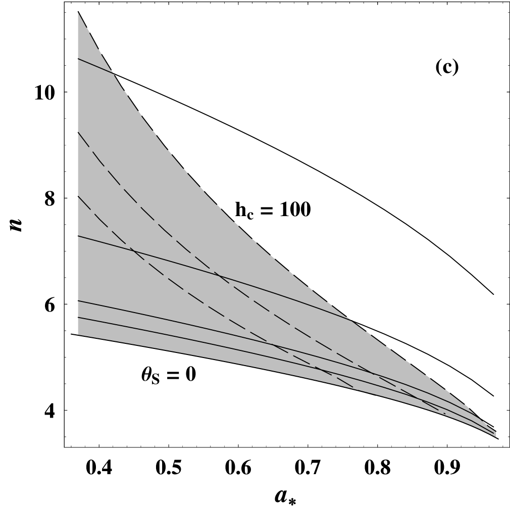
Figure 2: (a) The contours of $\theta_{S}\left({a_{*},n}\right)$ (solid lines); (b) the contours of $h_{c}\left({a_{*},n}\right)$ (dashed lines); (c) a shaded region for occurrence of SIMC and SIBZ bounded by the contours $\theta_{S}=0$ and $h_{c}=100$.

As argued in W04 the angle $\theta_{S}$ can be determined by the criterion of SIMC with the mapping relation between the BH horizon and the disk, and it is a function of the BH spin $a_{*}$ and the power-law index $n$, i.e., $\theta_{S}\left({a_{*},n}\right)$. Inspecting equations (1), (10) and (19), we find that $h_{c}$ is a dimensionless parameter also depending on the parameters $a_{*}$ and $n$, i.e., $h_{c}=h_{c}\left({a_{*},n}\right)$. By using equations (2) and (19) we have the contours of $\theta_{S}\left({a_{*},n}\right)$ and $h_{c}\left({a_{*},n}\right)$ in $a_{*}-n$ parameter space as shown in Figure 2.

Inspecting Figure 2, we find the following features of the contours:

(1) The values of $\theta_{S}$ increases and those of $h_{c}$ decreases with the increasing $n$ for the given BH spin $a_{*}$, respectively.

(2) The values of $\theta_{S}$ increases and those of $h_{c}$ decreases with the increasing $a_{*}$ for the given $n$, respectively.

(3) Both SIMC and SIBZ will occur, provided that the parameters $a_{*}$, $n$ and $h_{c}$ are greater than some critical values. As shown in Figure 2c the shaded region indicates the value ranges of $a_{*}$ and $n$ in which both $\theta_{S}>0$ and $h_{c}>100$ are constrained. Thus the occurrence of SIMC and SIBZ is guaranteed by the value ranges of $a_{*}$ and $n$ in the shaded region.

3 TIME SCALE OF A GRB AND ENERGY EXTRACTION FROM A ROTATING BH

There are several scenarios to invoke the BZ process for powering GRBs, and the main differences among these scenarios lie in the environment of a spinning BH and the approaches to the duration of a GRB. These scenarios are outlined as follows.

Model I: In Lee00 the energy is extracted magnetically from a rotating BH without disk, and the duration of a GRB is estimated as the time for extracting all rotational energy of the central BH via the BZ process.

Model II: It is argued that the energy is extracted magnetically from a rotating BH with a transient disk, and the duration of a GRB is estimated as the time for the disk plunged into the BH (Lee & Kim 2002; Wang et al. 2002).

Model III: In Li00 the energy is extracted magnetically from a rotating BH with a stationary torus in the state of suspended accretion, and the duration of a GRB is estimated roughly as the time for extracting all rotational energy of the central BH via the BZ process.

Model IV: In B00 the energy is extracted magnetically from a rotating BH with a non-stationary disk in the state of suspended accretion, and the duration of a GRB is determined by the presence of the disk.

Model V: In P03 the energy is extracted magnetically from a rotating BH with a torus in the state of suspended accretion, and the duration of a GRB is determined by the instability of the disk.

Model VI: In Lei05 the energy is extracted magnetically from a rotating BH with a thin disk in the state of suspended accretion, and the duration of a GRB is determined by the lifetime of the half-opening angle.

This Model: It is a modified version of Model VI, in which the effects of SIMC and SIBZ are taken into account. Compared with Model VI some features and advantages are given as follows.

(1) The magnetic field configuration in Model VI is built based on the conservation of the closed magnetic flux connecting the BH with the disk with the precedence over the open magnetic flux, resulting in the closed field lines connecting the half-open angle $\theta_{BZ}$ at horizon with the disk extending to infinity. In this Model, however, the closed field lines are confined by SIMC within a region of a limited radius $r_{{}_{S}}$ (about a few Schwarzschild radii as shown in Table 4), which is consistent with the collapsar model for GRBs-SNe.

(2) As argued in the next section, the variability time scales of the light curves of GRBs are modulated by two successive flares due to SIBZ.

The main features of the above models for GRBs are summarized in Table 1.

In Model VI the duration of a GRB is regarded as the lifetime of the half-opening angle $\theta_{BZ}$, which is based on the evolution of the rotating BH. The same procedure can be applied to this model except that the angle $\theta_{BZ}$ is replaced by $\theta_{S}$ arising from SIMC. It is found that the characteristics of the BH evolution in this model are almost the same as given in Model VI as shown by $a_{*}-n$ parameter spaces in Figure 3.

For several GRB-SNe, the observed energy $E_{\gamma}$ and duration $T_{90}$ can be fitted by adjusting the parameters $n$ and $B_{15}$. The energy $E_{SN}$ can be predicted as shown in Table 2, where the values of $n$, $B_{15}$ and $E_{SN}$ fitted to five GRBs invoking Model VI and this model are shown in the left and right sub-columns, respectively.

The fractions of extracting energy from a rotating BH via the BZ and MC processes are defined respectively as $f_{BZ}$ and $f_{MC}$, and they read

$$f_{BZ}=\frac{E_{BZ}}{E_{BZ}+E_{MC}},\quad f_{MC}=\frac{E_{MC}}{E_{BZ}+E_{MC}},$$ (20)

where $E_{BZ}$ and $E_{MC}$ are the energies extracting in the BZ and MC processes, respectively.

$$E_{BZ}=\int_{0}^{t_{BZ}}{P_{BZ}dt},\quad E_{MC}=\int_{0}^{t_{BZ}}{P_{MC}dt}.$$ (21)

In equation (21) $t_{BZ}$ is defined as the lifetime of the angle $\theta_{S}$, which can be calculated by the same procedure given in Lei05. The MC power in equation (21) is expressed as (W04)

$${P_{MC}}\mathord{\left/{\vphantom{{P_{MC}}{P_{0}}}}\right.\kern-1.2pt}{P_{0}}=2a_{*}^{2}\int_{\theta_{S}}^{\theta_{L}}{\frac{\beta\left({1-\beta}\right)\sin^{3}\theta d\theta}{2-\left({1-q}\right)\sin^{2}\theta}},$$ (22)

where the parameter $\beta\equiv{\Omega_{F}}\mathord{\left/{\vphantom{{\Omega_{F}}{\Omega_{{}_{H}}}}}\right.\kern-1.2pt}{\Omega_{{}_{H}}}={\Omega_{{}_{D}}}\mathord{\left/{\vphantom{{\Omega_{{}_{D}}}{\Omega_{{}_{H}}}}}\right.\kern-1.2pt}{\Omega_{{}_{H}}}$ is the ratio of the angular velocity of the magnetic field lines to that of the BH.

In Model VI the BH spin $a_{\ast}^{GRB}$ corresponds to the time when the half-opening angle $\theta_{BZ}=0$, and the BZ power $P_{BZ}=0$, while $a_{\ast}^{SN}$ corresponds to the MC power $P_{MC}=0$. In this model $a_{\ast}^{GRB}$ and $a_{\ast}^{SN}$ have the same meanings as given in Model VI except that $\theta_{BZ}$ is replaced by $\theta_{S}$.

As shown in Table 3, the values of $a_{\ast}^{GRB}$, $f_{BZ}$ and $f_{MC}$ fitted to five GRBs invoking Model VI and this model are shown in the left and right sub-columns, respectively.

Inspecting the data in the left and right sub-columns in Table 2 and Table 3, we find that $f_{BZ}$ and $f_{MC}$ in this model are greater and less than the counterparts in Model VI, respectively. This result arises from the effects of SIMC and SIBZ: the half-opening angle $\theta_{S}$ in this model is greater than the half-opening angle $\theta_{BZ}$ in Model VI as argued in W04.

4 AN EXPLANATION FOR VARIABILITIES IN GRB LIGHT CURVES

As is well known, the bursts are divided into long and short bursts according to their $T_{90}$. Most GRBs are highly variable, showing 100% variations in flux on a time scale much shorter than the overall duration of the burst. The bursts seem to be composed of individual pulses, with a pulse being the “building block” of the overall light curve. The variability time scale $\delta t$is much shorter than the GRBs’ duration $T_{90}$, the former is more than a factor of 10⁴ smaller than the latter (Piran, 2004). However, the origin of the variability in the light curves of GRBs remains unclear.

In this paper, we combine the variability with the screw instability of the magnetic field in the BH magnetosphere, and suggest that the variability could be fitted by a series of flares arising from SIBZ, which accompanies the release of the energy of the toroidal magnetic field.

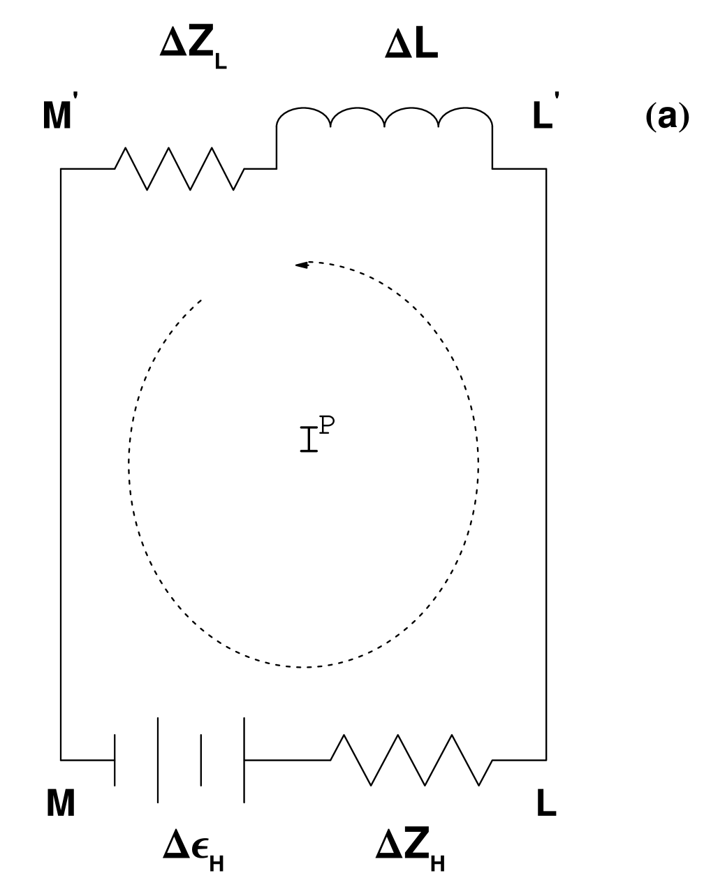
Figure 4: (a) An equivalent R-L circuit consisting of two magnetic surfaces, $M{M}^{\prime}$ and $L{L}^{\prime}$, which connect the BH horizon and the remote load; (b) a simplified configuration of poloidal magnetic field corresponding to the equivalent R-L circuit.

An equivalent circuit $ML{L}^{\prime}{M}^{\prime}$ for SIBZ is shown in Figure 4a, which consisting of two adjacent magnetic surfaces $M{M}^{\prime}$ and $L{L}^{\prime}$ connecting the BH horizon and the remote load. An inductor is introduced in the equivalent circuit by considering that the toroidal magnetic field threads the loop $ML{L}^{\prime}{M}^{\prime}$, and the inductor is represented by the symbol $\Delta L$ in Figure 4a.

The inductance $\Delta L$ in the circuit is defined by

$$\Delta L={\Delta\Psi^{T}}\mathord{\left/{\vphantom{{\Delta\Psi^{T}}{I_{L}}}}\right.\kern-1.2pt}{I_{L}},$$ (23)

where $I_{L}$ is given by equation (9), and $\Delta\Psi^{T}$ is the flux of the toroidal magnetic field threading the circuit. The flux $\Delta\Psi^{T}$ can be integrated over the loop $ML{L}^{\prime}{M}^{\prime}$ as follows,

$$\Delta\Psi^{T}=\oint_{loop}{B^{T}\sqrt{g_{rr}g_{\theta\theta}}dr}d\theta,$$ (24)

where the toroidal magnetic field measured by “zero-angular-momentum observers” is

$$B^{T}={2I_{L}}\mathord{\left/{\vphantom{{2I_{L}}{\left({\alpha\varpi}\right)}}}\right.\kern-1.2pt}{\left({\alpha\varpi}\right)},$$ (25)

where $\alpha$ is the lapse function defined in equation (1) (MT82).

Since the geometric shapes of the magnetic surfaces are unknown, we assume that the surfaces are formed by rotating the two radial segments $M{M}^{\prime}$ and $L{L}^{\prime}$, which span the angle $\Delta\theta$ as shown in Figure 4b. Thus the flux $\Delta\Psi^{T}$ can be calculated easily by integrating over the region $ML{L}^{\prime}{M}^{\prime}$. Incorporating equations (23)—(25), we obtain $\Delta L$as follows.

$$\Delta L=2\csc\theta\Delta\theta\int_{r_{H}}^{L_{BZ}}{{\rho^{2}dr}\mathord{\left/{\vphantom{{\rho^{2}dr}\Delta}}\right.\kern-1.2pt}\Delta}=2M\Delta\theta\csc\theta_{S}\int_{\left({1+q}\right)}^{{L_{BZ}}\mathord{\left/{\vphantom{{L_{BZ}}M}}\right.\kern-1.2pt}M}{\frac{\left({\tilde{r}^{2}+a_{*}^{2}\cos^{2}\theta_{S}}\right)}{\left({\tilde{r}^{2}+a_{*}^{2}-2\tilde{r}}\right)}d\tilde{r}},$$ (26)

where $\tilde{r}$ is defined as $\tilde{r}\equiv r\mathord{\left/{\vphantom{rM}}\right.\kern-1.2pt}M$.

Although the detailed process of SIBZ is still unclear, we suggest that the energy release in one event of SIBZ is roughly divided into two stages: the processes for releasing and retrieving magnetic energy, respectively. The two processes can be simulated as the corresponding processes in the equivalent$R-L$circuit. The detailed analysis is given as follows.

At the first stage the energy of the toroidal magnetic field is released as soon as SIBZ occurs, being dissipated on the load and plasma fluid in the way analogous to a discharging process in an equivalent $R-L$ circuit. The equation governing the discharging process in $R-L$ circuit is

$$\Delta L\frac{dI^{P}}{dt}+\left({\Delta Z_{PLSM}+\Delta Z_{L}}\right)I^{P}=0,$$ (27)

where $\Delta Z_{PLSM}$ is the resistance of the plasma fluid in the BH magnetosphere.

At the second stage the energy of toroidal magnetic field is recovered due to the rotation of the BH, and the process for retrieving magnetic energy is modulated by a charging process in an equivalent $R-L$ circuit. The equation governing the charging process in $R-L$ circuit is

$$\Delta L\frac{dI^{P}}{dt}+\left({\Delta Z_{H}+\Delta Z_{L}}\right)I^{p}=\Delta\varepsilon_{{}_{H}}.$$ (28)

In equations (27) and (28) $\Delta L$ is the inductance in the circuit $ML{L}^{\prime}{M}^{\prime}$, and $\Delta Z_{PLSM}$ is the resistance of the plasma in the BH magnetosphere. Incorporating equations (12) and (26), we have

$${\Delta L}\mathord{\left/{\vphantom{{\Delta L}{\Delta Z_{H}}}}\right.\kern-1.2pt}{\Delta Z_{H}}=\left({9.85\times 10^{-6}\sec}\right)\frac{\left({M\mathord{\left/{\vphantom{M{M_{\odot}}}}\right.\kern-1.2pt}{M_{\odot}}}\right)}{2-\left({1-q}\right)\sin^{2}\theta_{S}}\int_{\left({1+q}\right)}^{{L_{BZ}}\mathord{\left/{\vphantom{{L_{BZ}}M}}\right.\kern-1.2pt}M}{\frac{\left({\tilde{r}^{2}+a_{*}^{2}\cos^{2}\theta_{S}}\right)}{\left({\tilde{r}^{2}+a_{*}^{2}-2\tilde{r}}\right)}d\tilde{r}}.$$ (29)

Combining the initial conditions in the first and second stages, we have the solutions of equations (27) and (28) as follows,

$$I_{disch}^{p}=I_{initial}^{p}e^{-t\mathord{\left/{\vphantom{t{\tau_{1}}}}\right.\kern-1.2pt}{\tau_{1}}},$$ (30)

$$I_{ch}^{p}=I_{steady}^{p}\left({1-e^{-t\mathord{\left/{\vphantom{t{\tau_{2}}}}\right.\kern-1.2pt}{\tau_{2}}}}\right).$$ (31)

In equations (30) and (31) $I_{initial}^{p}$ and $I_{steady}^{p}$ are the initial and steady currents, respectively, while $I_{disch}^{p}$ and $I_{ch}^{p}$ represent the discharging and charging currents, respectively. The characteristic time scales in equations (30) and (31) are given respectively by $\tau_{1}$ and $\tau_{2}$, and they read

$$\tau_{1}\equiv{\Delta L}\mathord{\left/{\vphantom{{\Delta L}{\left({\Delta Z_{PLSM}+\Delta Z_{L}}\right)}}}\right.\kern-1.2pt}{\left({\Delta Z_{PLSM}+\Delta Z_{L}}\right)},$$ (32)

$$\tau_{2}\equiv{\Delta L}\mathord{\left/{\vphantom{{\Delta L}{\left({\Delta Z_{H}+\Delta Z_{L}}\right)}}}\right.\kern-1.2pt}{\left({\Delta Z_{H}+\Delta Z_{L}}\right)}.$$ (33)

From equations (32) and (33) we have the ratio of $\tau_{1}$ to $\tau_{2}$ given by

$${\tau_{1}}\mathord{\left/{\vphantom{{\tau_{1}}{\tau_{2}}}}\right.\kern-1.2pt}{\tau_{2}}={2\Delta Z_{H}}\mathord{\left/{\vphantom{{2\Delta Z_{H}}{\left({\Delta Z_{PLSM}+\Delta Z_{H}}\right)}}}\right.\kern-1.2pt}{\left({\Delta Z_{PLSM}+\Delta Z_{H}}\right)},$$ (34)

where $\Delta Z_{H}=\Delta Z_{L}$ is used in deriving equation (34).

In contrast to disk plasma of perfect conductivity, the resistance $\Delta Z_{PLSM}$ cannot be neglected based on the following considerations:

(1) The plasma fluid becomes very tenuous after leaving the inner edge of the disk, augmenting significantly the resistance due to an increasing radial velocity onto the BH;

(2) The conductivity of the plasma fluid is highly anisotropic, i.e., the conductivity in the cross-field direction is greatly impeded by the presence of the strong magnetic threading the BH (Punsly 2001).

Although the value of $\Delta Z_{PLSM}$ is unknown, we can estimate roughly the variability time scales of GRBs by combining equation (34) with different cases given as follows.

CASE I: $\Delta Z_{PLSM}>>\Delta Z_{H}$ leads to $\tau_{1}<<\tau_{2}$, and the time scale of two successive flares arising from SIBZ is dominated by $\tau_{2}$.

CASE II: $\Delta Z_{PLSM}\approx\Delta Z_{H}$ leads to $\tau_{1}\approx\tau_{2}$, and the time scale of two successive flares arising from SIBZ is about $2\tau_{2}$.

CASE III: $\Delta Z_{PLSM}<<\Delta Z_{H}$ leads to $\tau_{1}\approx 2\tau_{2}$, and the time scale of two successive flares arising from SIBZ is about $3\tau_{2}$.

Therefore the variability time scales are insensitive to the values of the unknown $\Delta Z_{PLSM}$. From equation (31) we obtain that the charging current attains 99.3% of $I_{steady}^{p}$ in the relax time $t_{relax}=5\tau_{2}$, implying the recovery of the toroidal magnetic field, and the variability time scales of GRBs can be estimated as follows,

$$\left({\delta t}\right)_{I}\equiv\left({t_{SIBZ}}\right)_{I}\approx 5\tau_{2},\quad for\quad\Delta Z_{PLSM}>>\Delta Z_{H},$$ (35)

$$\left({\delta t}\right)_{II}\equiv\left({t_{SIBZ}}\right)_{II}\approx 10\tau_{2},\quad for\quad\Delta Z_{PLSM}\approx\Delta Z_{H},$$ (36)

$$\left({\delta t}\right)_{III}\equiv\left({t_{SIBZ}}\right)_{III}\approx 15\tau_{2},\quad for\quad\Delta Z_{PLSM}<<\Delta Z_{H}.$$ (37)

In CASE I we have $\tau_{1}<<\tau_{2}$, implying that the magnetic energy is released much more rapidly in the first stage compared with the time for the recovery of the magnetic energy in the second stage. Thus CASE I seems more consistent with the feature of the light curves, i.e., an individual pulse is a fast-rise exponential decay (FRED) with an average rise-to-decay ratio of 1:3 (Norris et al. 1996).

By using equations (29), (33) and (35)—(37) we have the variability time scales in the light curves of four GRBs in the three different cases as shown in Table 4. In addition, we obtain the curves of $\left({\delta t}\right)_{I}$ versus $a_{*}$ with the fixed values of $n$ for GRB 990712, GRB 991208 and GRB 021216 as shown in Figure 5.

Inspecting Table 4, we find that the variability time scales of tens of msec in the light curves of GRBs can be modulated by the two successive flares due to SIBZ, which accompany the BZ process in powering the GRBs. We also find that the variability time scales of the four GRBs are generally three order of magnitude less than the corresponding durations $T_{90}$, which are consistent with the observations.

From Figure 5 we find that the curves of $\left({\delta t}\right)_{I}$ versus $a_{*}$ are almost the same, increasing linearly in a rather small slope with the decreasing $a_{*}$. The values of $\left({\delta t}\right)_{I}$ remains less than 20 msec during the occurrence of SIBZ for these GRBs.

5 DISCUSSION

5.1 Mechanism for the recurrent occurrence of SIBZ

In this paper we discuss the possibility of the modulations of SIBZ on the light curves of GRBs. One of the puzzles is what mechanism leads to the recurrent occurrence of SIBZ, and prevents the magnetic field from settling to a screw-stable configuration.

As argued in MT82 the BH magnetosphere consists of a series of magnetic surfaces connecting the horizon with the loads, and the total electric current $I$ flowing downward through an m-loop is proportional to the toroidal magnetic field $B^{T}$ by Ampere’s law. It is argued that these magnetic surfaces can be regarded as an equivalent circuit, in which each loop consists of two adjacent magnetic surfaces (W02). The total electric current flowing downward through an m-loop is exactly equal to the algebraic sum of the poloidal currents flowing in the loops (W03).

As shown in Figure 1 the critical magnetic surface (henceforth CMS) for SIBZ is represented by the critical line $M{M}^{\prime}$. According to the criterion (7) only the toroidal magnetic field outside CMS is depressed by SIBZ, while the toroidal and poloidal components of the magnetic field within CMS are little affected. On the other hand, the poloidal magnetic field outside CMS still exists in spite of the occurrence of SIBZ, and the toroidal magnetic field outside CMS will be recovered because of the twist of the poloidal magnetic field arising from the rotation of the BH. So, the rotation of the BH is the main mechanism for the recurrent occurrence of SIBZ in the BH magnetosphere.

5.2 Rotation period of BH and time scales of recovery of toroidal magnetic fields

If we take BH mass as 10$M_{\odot}$, the rotation period of the BH is only $\sim$1msec for the BH spin required by the criterion of SIBZ. This result implies that toroidal magnetic fields can not be recovered in one period of a rotating BH. How to explain the discrepancy between BH rotation and the time scales required for recovery of toroidal fields ?

In spite of lack of detailed knowledge of the screw instability, it is helpful to imagine the magnetic field line as an elastic string. The rotating BH always twists the field line, while the field line tries to untwist itself. Once the toroidal component of the magnetic field is strong enough to satisfy the criterion, the screw instability will occurs, just as a twisted elastic string releases its energy under appropriate conditions. In our model we simulate the process for twisting the field line by a transient process for accumulating magnetic energy in the inductor $\Delta L$ in the equivalent $R-L$ circuit, which corresponds to the increase of the toroidal magnetic field, and the variability time scales of tens of msec in the light curves of several GRBs are fitted as the time interval between two successive flares due to SIBZ. Thus the threshold of toroidal magnetic field (magnetic energy) cannot be recovered in only one rotation of BH, just as a threshold of twisting more than one turn is required for an elastic string to release its energy.

5.3 An explanation for GRBs with XRFs and XRRs

Recently, much attention has been paid to the issue of X-ray flashes (XRFs), X-ray-rich gamma-ray bursts (XRRs) and GRBs, since HETE-2 provided strong evidence that the properties of these three kinds of bursts form a continuum, and therefore these objects are probably the same phenomenon (Lamb et al. 2004a, 2004b, 2005). The observations from HETE-2 motivate some authors to seek a unified model of these bursts. The most competitive unified models of these bursts are off-axis jet model (Yamazaki, Ioka, & Nakamura 2002; Lamb et al. 2005) and two-component jet model (Berger et al. 2003; Huang et al. 2004), in which XRFs, XRRs and GRBs arise from the differences in the viewing angles. Unfortunately, a detailed discussion on producing different viewing angles for XRFs, XRRs and GRBs has not been given in the above works.

Our argument on SIBZ and SIMC may be helpful to understanding this issue. It is believed that a disk is probably surrounded by a high-temperature corona analogous to the solar corona (Liang & Price 1977; Haardt 1991; Zhang et al 2000). Very recently, some authors argued that the coronal heating in some stars including the Sun is probably related to dissipation of currents, and very strong X-ray emissions arise from variation of magnetic fields (Galsgaard & Parnell 2004; Peter et al. 2004). Analogously, if the corona exists above the disk in our model, we expect that it might be heated by the induced currents due to SIMC and SIBZ. Therefore a very strong X-ray emission would be produced to form XRFs or XRRs.

Although our model may be too simplified and idealized with respect to the real situation, it provides a possible scenario for the occurrence of the screw instability in BH magnetosphere, and it may be helpful to understanding some astrophysical observations. We hope to improve our model by combining more observations in the future.

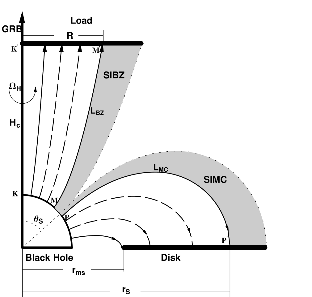
Figure 1: A schematic drawing for magnetic field configuration with screw instability in BH magnetosphere, where the screw-unstable regions for SIBZ and SIMC are indicated by the shaded regions (not in scale).

Figure 3: BH evolution is described in $a_{*}-n$ parameter space with and without screw instability in (a) and (b), respectively. The parameter space is divided by the contours of $\tilde{P}_{BZ}=0$, that of $\tilde{P}_{MC}=0$ and that of $A=0$ into several sub-regions. The duration of a GRB is regarded as the time for the represent point of BH evolution moving from its initial position in region IA to the contour $\tilde{P}_{BZ}=0$. The dimensionless BZ and MC powers are defined as $\tilde{P}_{BZ}\equiv P_{BZ}/P_{0}$ and $\tilde{P}_{MC}\equiv P_{MC}/P_{0}$, respectively. The function $A=A(a_{\ast},n)$ is given in Lei05, being proportional to the rate of change of the BH spin.

Figure 5: The curves of $\left({\delta t}\right)_{I}$ versus $a_{*}$ with n =3.54, 3.55 and 3.58 for GRBs 990712, 991208 and 991216 in (a), (b) and (c), respectively.

Table 1: The Main Features of Several Models Invoking the BZ Process For Powering GRBs

Model	BZ Process	MC Process	Surrounded By	Objects	Half-Opening Angle	Variability
I	Yes	No	No disk	GRB	No	No
II	Yes	No	Transient Disk	GRB	No	No
III	Yes	No	Torus	GRB	No	No
IV	Yes	Yes	Disk	GRB/SN	No	No
V	Yes	Yes	Torus	GRB/SN	Yes	No
VI	Yes	Yes	Disk	GRB/SN	Yes	No
This Model	Yes	Yes	Disk	GRB/SN	Yes	Yes

Table 2: Five GRBs of True Energy $E_{\gamma}$ and $T_{90}$s Fitted with Different Power-law Index $n$ and $B_{H}$ with the Predicted $E_{SN}$.

GRBa	$E_{\gamma}^{b}$	$T_{90}$	$n$		$B_{15}^{h}$		$E_{SN}^{c}$
970508	0.234	15d	3.89	3.46	0.97	0.70	1.947	1.732
990712	0.445	30e	3.98	3.54	0.81	0.61	1.989	1.816
991208	0.455	39.84f	3.99	3.55	0.75	0.56	1.995	1.817
991216	0.695	7.51f	4.06	3.58	1.80	1.40	2.032	1.887
021211	0.117	13.3g	3.81	3.42	0.9	0.6	1.901	1.681

Note. —

^aThis sample of GRB-SNe is taken from Table 1 of Dar (2004).

^bThe true energies $E_{\gamma}$ of the GRBs are given in terms of $10^{51}ergs$ from Table 1 of Frail et al (2001).

^cThe predicted energies $E_{SN}$ of the SNe are given in terms of $10^{51}ergs$ based our models.

^dThe duration of GRB 970508 is from Costa et al. (1997).

^eThe duration of GRB 990712 is from Heise et al. (1999).

^fThe durations of GRBs 991208 and 991216 are from Table 2 of Lee & Kim (2002).

^gThe duration of GRB 021211 is from Sakamoto et al. (2005).

^h$B_{15}$ is the magnetic field at the BH horizon in terms of $10^{15}gauss$. The initial BH spin is assumed to be $a_{\ast}(0)=0.9$, and the data in the left and right sub-columns of the parameters $n$ and $B_{15}$ and $E_{SN}$ are calculated based on Model VI and this model, respectively.

Table 3: Five GRBs Fitted with Different $f_{BZ}$ and $f_{MC}$ Invoking Model VI and This model.

GRB	$a_{\ast}^{GRB}$		$f_{BZ}$		$f_{MC}$		$a_{\ast}^{SN}$
970508	0.798	0.871	0.009	0.020	0.991	0.980	0.233	0.226
990712	0.767	0.853	0.014	0.028	0.986	0.972	0.234	0.227
991208	0.763	0.852	0.014	0.029	0.986	0.971	0.235	0.227
991216	0.736	0.842	0.019	0.032	0.981	0.968	0.236	0.228
021211	0.823	0.880	0.006	0.016	0.994	0.984	0.232	0.225

Table 4: Variability Time Scale in the Light-Curves of Five GRBs.

GRBs		Parameters			$T_{90}$(s)		Variablity Time scale (ms)
	$a_{*}$	$n$	$\tilde{r}_{S}$	$h_{c}$		$\left({\delta t}\right)_{I}$	$\left({\delta t}\right)_{II}$	$\left({\delta t}\right)_{III}$
970508	0.9	3.46	5.96	87.71	15	13.42	26.84	40.25
990712	0.9	3.54	6.45	85.56	30	13.23	26.46	39.68
991208	0.9	3.55	6.52	87.71	39.84	13.42	26.84	40.25
991216	0.9	3.58	6.77	87.70	7.51	13.42	26.83	40.25
021211	0.9	3.42	5.77	59.32	13.3	10.90	21.80	32.70

Note. —

$\tilde{r}_{S}\equiv{r_{{}_{S}}}\mathord{\left/{\vphantom{{r_{{}_{S}}}M}}\right.\kern-1.2pt}M$ is the critical dimensionless radius for SIMC.

References

- (1) Bateman, G. 1978, MHD Instabilities (Cambridge: MIT)
- (2) Berger, E., et al., 2003, Nature, 426, 154
- (3) Blandford, R. D., 1999, in ASP Conf. Ser. 160, Astrophysical Discs: An EC Summer School, ed. J. A. Sellwood & J. Goodman (San Francisco: ASP), 265
- (4) Blandford, R. D., & Znajek, R. L. 1977, MNRAS, 179, 433
- (5) Bloom, J. S. et al. 1999, Nature, 401, 453
- (6) Brown, G. E., et al. 2000, New Astronomy 5, 191 (B00)
- (7) Costa, E., et al. 1997, IAUC Circ. No. 6649
- (8) Dar, A. 2004, preprint (astro-ph/0405386)
- (9) Frail, D. A., et al. 2001, ApJ, 562, L55
- (10) Galama, T. J., et al. 1998, Nature, 395, 672
- (11) —. 2000, ApJ, 536, 185
- (12) Galsgaard, K., & Parnell, C., Procedings of SOHO 15 Coronal Heating, ESA publication, preprint (astro-ph/0409562)
- (13) Gruzinov, A. 1999, preprint (astro-ph/9908101)
- (14) Haardt F., & Maraschi L., 1991, ApJ, 380, L51
- (15) Hjorth, J., et al. 2003, Nature, 423, 847
- (16) Hoflich, P. J., Wheeler, J. C., & Wang, L. 1999, ApJ, 521, 179
- (17) Huang, Y. F., et al., 2004, ApJ, 605, 300
- (18) Kadomtsev, B. B. 1966, Rev. Plasma Phys., 2, 153
- (19) Lamb, D. Q. et al. 2004a, NewAR, 48, 423
- (20) Lamb, D. Q., Donaghy, T. Q., & Graziani, C., 2004b, NewAR, 48, 459
- (21) —. 2005, ApJ, 620, 355
- (22) Lee, H. K., Wijers, R. A. M. J., & Brown, G. E. 2000, Phys. Rep., 325, 83 (Lee00)
- (23) Lee, H. K., & Kim, H. K. 2002, J. Korean Phys. Soc. 40, 524
- (24) Lei, W.-H., Wang, D.-X., & Ma, R.-Y. 2005, ApJ, 619, 420 (Lei05)
- (25) Li, L. -X. 2000a, ApJ, 531, L111
- (26) —. 2000b, ApJ, 533, L115
- (27) —. 2000c, ApJ, 544, L375 (Li00)
- (28) —. 2002, ApJ, 567, 463
- (29) Liang E. P. T., & Price R. H., 1977, ApJ, 218, 247
- (30) MacDonald, D., & Thorne, K. S. 1982, MNRAS, 198, 345 (MT82)
- (31) McBreen, S., Quilligan, F., McBreen, B., Hanlon, L., & Watson, D., 2001, A&A, 380, L31.
- (32) Nakar, E., & Piran, T., 2002, MNRAS, 331, 40
- (33) Norris et al., ApJ 1996, 459, 393
- (34) Novikov, I. D., & Thorne, K. S., 1973, in Black Holes, ed. Dewitt C, (Gordon and Breach, New York) p.345
- (35) Peter, H., Gudiksen, B., & Nordlund, A., 2004, ApJ, 617, 85
- (36) Piran, T., Rev. Mod. Phys., 2004, 76, 1143
- (37) Punsly, B. 2001, Black Hole Gravitohydromagnetics (Springer-Verlag, New York)
- (38) Sakamoto, T. et al., 2005, ApJ, 629, 311
- (39) Stanek, K. Z. et al. 2003, ApJ, 591, L17
- (40) van Putten, M. H. P. M. 1999, Science, 284, 115
- (41) —. 2001, Phys. Rep., 345, 1
- (42) van Putten, M. H. P. M., & Levinson, A. 2003, ApJ, 584, 937 (P03)
- (43) van Putten, M. H. P. M., & Ostriker, E. C. 2001, ApJ, 552, L31
- (44) Wang, D.-X., Xiao, K., Lei, W.-H. & Ma, R.-Y., 2002, MNRAS, 335, 655 (W02)
- (45) Wang, D.-X., Lei, W.-H., Xiao, K., & Ma, R.-Y., 2002, ApJ, 580, 358
- (46) Wang, D.-X., Ma, R.-Y., Lei, W.-H., & Yao, G.-Z. 2003, ApJ, 595, 109 (W03)
- (47) —.2004, ApJ, 601, 1031 (W04)
- (48) Yamazaki, R., Ioka K., & Nakamura T., 2002, ApJ, 571, L31
- (49) Zhang S. N. et al., 2000, Science, 287, 1239