Magellanic Cloud Structure from Near-IR Surveys I:
The Viewing Angles of the LMC

Abstract

We present a detailed study of the viewing angles of the LMC disk plane. We find that our viewing direction differs considerably from the commonly accepted values, which has important implications for the structure of the LMC.

The discussion is based on an analysis of spatial variations in the apparent magnitude of features in the near-IR color-magnitude diagrams extracted from the DENIS and 2MASS surveys. Sinusoidal brightness variations with a peak-to-peak amplitude of $\sim 0.25$ mag are detected as function of position angle. The same variations are detected for AGB stars (using the mode of their luminosity function) and for RGB stars (using the tip of their luminosity function), and these variations are seen consistently in all of the near-IR photometric bands in both DENIS and 2MASS data. The observed spatial brightness variations are naturally interpreted as the result of distance variations, due to one side of the LMC plane being closer to us than the opposite side. There is no evidence that any complicating effects, such as possible spatial variations in dust absorption or the age/metallicity of the stellar population, cause large-scale brightness variations in the near-IR at a level that exceeds the formal errors ($\sim 0.03$ mag). The best fitting geometric model of an inclined plane yields an inclination angle $i=34.7^{\circ}\pm 6.2^{\circ}$ and line-of-nodes position angle $\Theta=122.5^{\circ}\pm 8.3^{\circ}$. The quoted errors are conservative estimates that take into account the possible influence of systematic errors; the formal errors are much smaller, $0.7^{\circ}$ and $1.6^{\circ}$, respectively. There is tentative evidence for variations of $\sim 10^{\circ}$ in the viewing angles with distance from the LMC center, suggesting that the LMC disk plane may be warped.

Traditional methods to estimate the position angle of the line of nodes have used either the major axis position angle $\Theta_{\rm maj}$ of the spatial distribution of tracers on the sky, or the position angle $\Theta_{\rm max}$ of the line of maximum gradient in the velocity field, given that for a circular disk $\Theta_{\rm maj}=\Theta_{\rm max}=\Theta$. The present study does not rely on the assumption of circular symmetry, and is considerably more accurate than previous studies of its kind. We find that the actual position angle of the line of nodes differs considerably from both $\Theta_{\rm maj}$ and $\Theta_{\rm max}$, for which measurements have fallen in the range $140^{\circ}$–$190^{\circ}$. This indicates that the intrinsic shape of the LMC disk is not circular, but elliptical. Paper II of this series explores the implications of this result through a detailed study of the shape and structure of the LMC. The inclination angle inferred here is consistent with previous estimates, but this is to some extent a coincidence, given that also for the inclination angle most previous estimates were based on the incorrect assumption of circular symmetry.

1 Introduction

The Large Magellanic Cloud (LMC) is our close neighbor. It plays a key role in determinations of the cosmological distance scale (e.g., Mould et al. 2000) and is used to study the presence of dark objects in the Galactic Halo through microlensing (e.g., Alcock et al. 2000b; Lasserre et al. 2000; Udalski et al. 1999). It is also of fundamental importance for all studies of stellar populations and the interstellar medium (see the book on the Magellanic Clouds by Westerlund 1997). For all these applications it is essential to have a good understanding of the overall structure of the LMC as a galaxy, which is the topic of the present series of papers.

The generally accepted consensus is that the LMC is a disk galaxy with an approximately planar geometry (the evidence for this is reviewed in Section 9.3). The most basic parameters in our understanding of the LMC are therefore the angles that describe the direction from which we are viewing the LMC plane: the inclination angle $i$ and the position angle $\Theta$ of the line of nodes (the intersection of the galaxy plane and the sky plane). It is remarkable that our knowledge of these parameters is only quite rudimentary, given that the LMC is easily visible with the naked eye and is many times the size of the full moon. The previous work on the LMC viewing geometry is summarized in Table 3.5 of Westerlund (1997). The quoted results for $i$ and $\Theta$ easily span a range of $25^{\circ}$ each, even if one restricts the discussion to the most reliable studies.

The large majority of all previous studies of the LMC viewing geometry have estimated the viewing angles under the assumption that the LMC disk is circular, using either the spatial distribution of tracers on the sky (as reviewed in Section 11.1) or their kinematics (as reviewed in Section 11.2). The obvious disadvantage of this approach is that there is no evidence that the LMC is indeed circular. To the contrary, all available evidence seems to indicate that the LMC is a highly complicated system with none of the characteristic symmetries that are often seen in spiral galaxies. Its interaction with the Small Magellanic Cloud (SMC) and the Galactic tidal field (e.g., Putman et al. 1998) may be partly responsible for this. The LMC hosts a central bar that is offset from the center of the outer isophotes; the HI rotation center coincides with neither (Westerlund 1997). The principal axes of the HI velocity field are not perpendicular, and the zero-velocity curve twists by $\sim 20^{\circ}$ from small to large radii (Kim et al. 1998). So it seems reasonable to worry about the accuracy of viewing angles inferred under the assumption of circular symmetry.

A more robust way to determine the LMC viewing angles is to use geometrical considerations without making assumptions about the distribution or kinematics of tracers in the LMC plane. This is possible, because the inclination of the LMC causes one side of it to be closer to us than the other. As a result, tracers on one side of the LMC should appear brighter than those on the other side. This is not a subtle effect, but should amount to $\sim 0.2$–$0.4$ mag for the viewing angles that are commonly quoted in the literature (as discussed in Section 2). This method does not rely on absolute distances or magnitudes, which are notoriously difficult to estimate, but only on relative distances or magnitudes. What has been lacking most is a large enough sample of stars to apply the method to. Cepheids have yielded results, but so far only with large error bars (as reviewed in Section 11.3).

Large-area digital surveys such as the Magellanic Cloud Photometric Survey (Zaritsky, Harris & Thompson 1997), DENIS (Epchtein et al. 1997) and the Two Micron All Sky Survey (2MASS; e.g., Skrutskie 1998) are now providing important new tools to analyze the LMC structure. In particular, the LMC viewing geometry can be constrained by studying how the apparent magnitude of well-defined features in the color-magnitude diagram (CMD) varies as a function of position in the LMC. A similar technique has been used to study the inclination of the bar in the Milky Way (e.g., Stanek et al. 1994). Weinberg & Nikolaev (2000) applied this technique to the LMC, using Asymptotic Giant Branch (AGB) stars selected from the 2MASS survey, but they did not pursue this issue in as much detail as we do here (as discussed in Section 11.4).

In this first paper of a series on LMC structure we analyze the LMC viewing angles by studying how the characteristic apparent magnitudes of AGB and Red Giant Branch (RGB) stars vary with position in the LMC. The analysis is restricted to stars in the outer parts of the LMC, $\geq 2.5^{\circ}$ from the LMC center. The analysis is based primarily on the $I$, $J$ and $K_{s}$ band data from the DENIS survey, and in particular the data collected in the DENIS Catalog towards the Magellanic Clouds (DCMC; Cioni et al. 2000a). However, 2MASS data are used as well. Section 2 presents the theoretical basis of the analysis. Coordinate systems are introduced, and it is derived how brightness variations on the sky are related to the LMC viewing geometry. Section 3 describes the method used for the analysis of near-infrared (near-IR) CMDs. Section 4 discusses the technique for data-model comparison to obtain estimates for the viewing angles from the data. Section 5 presents the results of an analysis of the $I$-band magnitudes of AGB stars selected by $I-J$ color. Section 6 addresses the extent to which the results of this analysis depend on the photometric band(s) used for the analysis or the color selection. Section 7 compares the spatial variations in the brightness of the tip of the RGB (TRGB) with the results obtained for AGB stars. Section 8 studies variations in the characteristic magnitudes of AGB stars with distance from the LMC center. Section 9 provides a detailed assessment of possible sources of systematic error, including spatial variations in dust absorption or the age/metallicity of the stellar population. Also, results from DENIS and 2MASS data are compared to assess the influence of possible systematic errors in the data. Section 10 studies the dependence of the viewing angles on the distance from the LMC center, which constrains warps and twists of the LMC disk plane. Section 11 discusses how the inferred viewing angles compare to the results of previous authors. Section 12 addresses the implications for the relative positions and distances of some well-studied objects, supernova SN1987A and two eclipsing binaries, with respect to the LMC center. Section 13 presents concluding remarks. Appendix A discusses the photometric accuracy of the DCMC, and discusses improvements made to the photometric zeropoint calibrations of Cioni et al. (2000a).

Paper II of this series (van der Marel 2001a) studies the intrinsic shape and structure of the LMC, by combining the observed number density distribution of stars inferred from the 2MASS and DENIS surveys with the viewing angles inferred here. Paper III (van der Marel 2001b) addresses the question whether the structures in the central $2.5^{\circ}$, including the LMC bar, lie in the same plane as that defined by the outer disk.

2 Theoretical Framework

2.1 Angular Coordinates

The position of any point in space is uniquely determined by its right ascension (RA) and declination (DEC) on the sky, $(\alpha,\delta)$, and its distance $D$. A particular point ${\cal O}$ with coordinates $(\alpha_{0},\delta_{0},D_{0})$ is taken to be the origin of the analysis. This point will typically be chosen to be the center of the LMC, but the formulae that follow are valid more generally.

Angular coordinates $(\rho,\phi)$ are defined on the celestial sphere, where $\rho$ is the angular distance between the points $(\alpha,\delta)$ and $(\alpha_{0},\delta_{0})$, and $\phi$ is the position angle of the point $(\alpha,\delta)$ with respect to $(\alpha_{0},\delta_{0})$. In particular, $\phi$ is the angle at $(\alpha_{0},\delta_{0})$ between the tangent to the great circle on the celestial sphere through $(\alpha,\delta)$ and $(\alpha_{0},\delta_{0})$, and the circle of constant declination $\delta_{0}$. By convention, $\phi$ is measured counterclockwise starting from the axis that runs in the direction of decreasing RA at constant declination $\delta_{0}$.

The cosine rule of spherical trigonometry (e.g., Smart 1977) can be used to derive that

$$\cos\rho=\cos\delta\cos\delta_{0}\cos(\alpha-\alpha_{0})+\sin\delta\sin\delta_{0}.$$ (1)

Also, the sine rule of spherical trigonometry can be used to show that

$$\sin\rho\cos\phi=-\cos\delta\sin(\alpha-\alpha_{0}),$$ (2)

and the so-called analogue formula implies that

$$\sin\rho\sin\phi=\sin\delta\cos\delta_{0}-\cos\delta\sin\delta_{0}\cos(\alpha-\alpha_{0}).$$ (3)

These formulae uniquely define $(\rho,\phi)$ as function of $(\alpha,\delta)$, for a fixed choice of the origin ${\cal O}$.

It is often useful to plot observations on the celestial sphere on a flat piece of paper. This requires transformation equations from $(\alpha,\delta)$ to a cartesian coordinate system $(X,Y)$. We will use

$$X(\alpha,\delta)\equiv\rho\cos\phi,\qquad Y(\alpha,\delta)\equiv\rho\sin\phi.$$ (4)

This so-called ‘zenithal equidistant projection’ provides just one of the many possible ways of projecting a sphere onto a plane (see, e.g., Calabretta 1992).

2.2 Relative Distances and Magnitudes

A cartesian coordinate system $(x,y,z)$ is introduced that has its origin at ${\cal O}$, with the $x$-axis anti-parallel to the RA axis, the $y$-axis parallel to the declination axis, and the $z$-axis towards the observer. This yields the following transformations:

$$x = D\sin\rho\cos\phi,$$

$$y = D\sin\rho\sin\phi,$$ (5)

$$z = D_{0}-D\cos\rho.$$

If necessary, these equations can be expressed in terms of $(\alpha,\delta)$ using equations (1)–(3) (see also Appendix A of Weinberg & Nikolaev 2000).

A second cartesian coordinate system $(x^{\prime},y^{\prime},z^{\prime})$ is introduced that is obtained from the system $(x,y,z)$ by counterclockwise rotation around the $z$-axis by an angle $\theta$, followed by a clockwise rotation around the new $x^{\prime}$-axis by an angle $i$. With this definition, the $(x^{\prime},y^{\prime})$ plane is inclined with respect to the sky by the angle $i$ (with face-on viewing corresponding to $i=0$). The angle $\theta$ is the position angle of the line of nodes (the intersection of the $(x^{\prime},y^{\prime})$-plane and the $(x,y)$-plane of the sky), measured counterclockwise from the $x$-axis. In practice, $i$ and $\theta$ will be chosen such that the $(x^{\prime},y^{\prime})$ plane coincides with the plane of the LMC disk, but the formulae that follow are valid more generally. The transformations between the $(x^{\prime},y^{\prime},z^{\prime})$ and $(x,y,z)$ coordinates are:

$$x^{\prime} = x\cos\theta+y\sin\theta,$$

$$y^{\prime} = -x\sin\theta\cos i+y\cos\theta\cos i-z\sin i,$$ (6)

$$z^{\prime} = -x\sin\theta\sin i+y\cos\theta\sin i+z\cos i.$$

Substitution of equation (2.2) yields

$$x^{\prime} = D\sin\rho\cos(\phi-\theta),$$

$$y^{\prime} = D[\sin\rho\cos i\sin(\phi-\theta)+\cos\rho\sin i]-D_{0}\sin i,$$ (7)

$$z^{\prime} = D[\sin\rho\sin i\sin(\phi-\theta)-\cos\rho\cos i]+D_{0}\cos i.$$

Here the elementary rules $\cos(\phi-\theta)=\cos\phi\cos\theta+\sin\phi\sin\theta$ and $\sin(\phi-\theta)=\sin\phi\cos\theta-\cos\phi\sin\theta$ were used, which follow from the complex identity $e^{i(\phi-\theta)}=e^{i\phi}e^{-i\theta}$.

One is interested in the distance $D$ of points in the $(x^{\prime},y^{\prime})$ plane, as function of the position $(\rho,\phi)$ on the sky. The points in this plane have $z^{\prime}=0$, so that equation (2.2) yields:

$$D/D_{0}=\cos i\>/\>[\cos i\cos\rho-\sin i\sin\rho\sin(\phi-\theta)].$$ (8)

This general equation simplifies in a number of special cases. If one considers points along the line of nodes, or if the system is viewed face on, then

$$D/D_{0}=1/\cos\rho\qquad({\rm for}\>\>\phi=\theta,\>\>\phi=\theta+180^{\circ},\>\>{\rm or}\>\>i=0).$$ (9)

On the other hand, if one considers points along a line that is perpendicular to the line of nodes then

$$D/D_{0}=\cos i/\cos(i\pm\rho)\qquad({\rm for}\>\>\phi=\theta\pm 90^{\circ}),$$ (10)

which uses the elementary rule that $\cos(i\pm\rho)=\cos i\cos\rho\mp\sin i\sin\rho$. For a fixed angular distance $\rho$ from the origin ${\cal O}$, the points with $\phi=\theta\pm 90^{\circ}$ are the ones for which $D/D_{0}$ reaches its maximum and minimum values, respectively. For small angular distances $\rho$ one can expand equation (8) using a Taylor expansion to obtain that

$$D/D_{0}=1+\rho\tan i\sin(\phi-\theta)+{\cal O}(\rho^{2}),\qquad(\rho\>\>{\rm in}\>\>{\rm radians,}\>\>\rho\ll 1).$$ (11)

In practice one does not directly have access to distances, but one does have access to stellar magnitudes. Consider identical objects at positions $(\alpha,\delta)$ and $(\alpha_{0},\delta_{0})$. The apparent magnitudes of these objects will differ by

$$\mu\equiv m-m_{0}=5\log(D/D_{0}).$$ (12)

The same will hold for the average magnitudes of groups of objects with identical properties. In general, $\mu$ can be evaluated as function of $(\rho,\phi)$ (i.e., position on the sky) using equation (8), for any given viewing angles $(i,\theta)$. For small angular distances $\rho$, one can use equation (11) and make a further Taylor expansion of the logarithm to obtain

$$\mu=\Big{(}{{5\,\pi}\over{180\ln 10}}\Big{)}\>\rho\tan i\sin(\phi-\theta)+{\cal O}(\rho^{2}),\qquad(\rho\>\>{\rm in}\>\>{\rm degrees,}\>\>\rho\ll 180/\pi),$$ (13)

where the angular distance $\rho$ is now expressed in degrees, to make it easier to assess the size of the magnitude difference for realistic situations. The constant in the equation is $(5\pi)/(180\ln 10)=0.038$ magnitudes. Hence, the magnitude at fixed $\rho$ has an approximately sinusoidal variation with position angle $\phi$, with amplitude $0.038\>\rho\tan i$. Stars in the LMC can be traced to radii $\rho$ of 5–10 degrees from the center, and previous analyses have suggested that $i\approx 45^{\circ}$ (so that $\tan i\approx 1$; e.g., Westerlund 1997). Hence, in the LMC one expects distance-related magnitude variations up to several tenths of a magnitude (much larger than typical observational errors). At fixed $\rho$, the magnitude variation $\mu$ always reaches its extrema at angles perpendicular to the line of nodes, $\phi=\theta\pm 90^{\circ}$. Figure 1 shows $\mu$ as function of $\rho$ along this line, for different values of the inclination $i$, as calculated from equations (10) and (12). For comparison, the heavy long-dashed line shows the linear approximation given by equation (13), for $i=40^{\circ}$.

2.3 Position angles

The usual method of measuring position angles in astronomy is to measure counterclockwise, starting from the North. By contrast, the angles $\phi$ and $\theta$ defined above are measured counterclockwise starting from the West. It is therefore useful to define

$$\Phi=\phi-90^{\circ},\qquad\Theta=\theta-90^{\circ},$$ (14)

which are the position angle of a point in the LMC and the position angle of the line-of-nodes, respectively, now measured with the usual astronomical convention.

The description of the LMC viewing geometry using the angle $\Theta$ can lead to some confusion, since the angle $\Theta$ is defined modulo $2\pi$, whereas the line-of-nodes is a line, and can therefore be described by two different position angles that differ by $\pi$. The definition used here corresponds to the usual convention (e.g., Westerlund 1997), by which the quantity referred to as the ‘position angle of the line-of-nodes’ (i.e., $\Theta$) is defined such that points in the direction of position angle $\Theta_{\rm near}\equiv\Theta-90^{\circ}$ are closer to the observer than those in the direction of position angle $\Theta_{\rm far}\equiv\Theta+90^{\circ}$.

3 Methodology to Constrain the LMC Structure from Near-IR Photometry

3.1 The DENIS Data

We study the apparent magnitude of well-defined features in the CMD as function of position in the LMC to determine the viewing angles using the formulae of Section 2. Large-scale digital surveys such as the Magellanic Cloud Photometric Survey (Zaritsky et al. 1997), DENIS (Epchtein et al. 1997) and 2MASS (e.g., Skrutskie 1998) are now yielding catalogs with up to millions of stars, which are ideally suited for a study of this nature.

In the present paper the discussion is restricted mostly to the near-IR data from the DENIS survey, and in particular to the data collected in the DENIS Catalog towards the Magellanic Clouds (DCMC; Cioni et al. 2000a). We used the latest version, which includes the data for the few scan strips missing from the first release. The resulting catalog has complete coverage over the LMC area with $4^{\rm h}\>06^{\rm m}\>\leq$ RA $\leq 6^{\rm h}\>47^{\rm m}\>$ and $-77^{\circ}\leq$ DEC $\leq-61^{\circ}$ (see Figure 4 below). It contains stellar magnitudes of sources detected in at least two of the three DENIS bands ($I$, $J$ and $K_{S}$). For the present analysis all sources in the catalog were used. Sources with non-optimal values of any of the DCMC data-quality flags were not excluded to optimize the statistics of the sample (several tests were performed to verify that this does not degrade the accuracy of the final results). An improved calibration of the photometric zeropoints for the individual DENIS scan strips was performed. This significantly increased the accuracy of the DCMC, as discussed in Appendix A. Systematic errors in the resulting stellar magnitudes are believed to be no larger than $\sim 0.02$ mag, i.e., much smaller than the expected distance-induced magnitude variations (cf. Figure 1). The issue of possible systematic errors is further addressed in Section 9.6, among other things by comparison to 2MASS data.

3.2 Near-IR Color Magnitude Diagrams

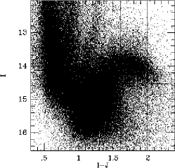
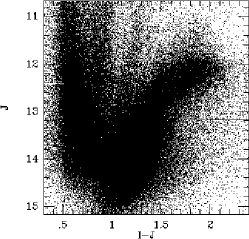
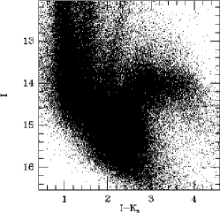
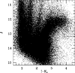
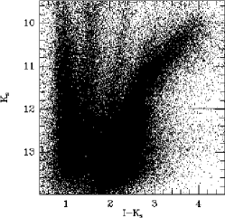
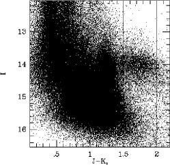
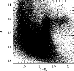
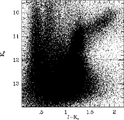
Figure 2: The panels show the nine independent CMDs that can be constructed from the $I$, $J$ and $K_{S}$ magnitudes obtained from the DENIS Survey. Each panel shows all the stars in the LMC area of the sky covered by the DCMC that were detected in all 3-bands. The features in the CMDs are discussed in the text. The horizontal bar at the right axis of each panel indicates the magnitude of the Tip of the Red Giant Branch (TRGB), as determined by Cioni et al. (2000c). The vertical lines in the top left panel indicate the range of $I-J$ colors that will be used for the main analysis of the present paper. The $I$-band LF of the stars with magnitudes in this color range is shown in Figure 3. The vertical lines in the bottom left panel show a range of $J-K_{s}$ colors that is used as a consistency check in Section 6.

Figure 2 shows the nine CMDs that can be generated from the $I$, $J$ and $K_{S}$ data in the DCMC. The general features of these near-IR CMDs of the LMC have been previously discussed by Cioni et al. (2000a,b,c). Detailed discussions of the near-IR $(J-K_{s},K_{s})$ and optical $(V-R,V)$ CMDs of the LMC have been presented by Nikolaev & Weinberg (2000) and Alcock et al. (2000a), respectively. We therefore summarize here only the main features of the CMDs in Figure 2, as relevant in the present context.

LMC stars in the RGB evolutionary phase are responsible for the pronounced feature that extends downward, slanted somewhat to the left, from the center of each CMD panel in Figure 2. The horizontal bar at the right axis of each panel indicates the magnitude of the Tip of the Red Giant Branch (TRGB), as determined by Cioni et al. (2000c). LMC stars in the AGB evolutionary phase are responsible for feature(s) at magnitudes that are brighter and redder than the TRGB. There are two main types of AGB stars, namely the oxygen-rich (O-rich) and the carbon-rich (C-rich) AGB stars. In the CMDs involving the $J-K_{s}$ color (bottom panels in Figure 2) these families separate into easily distinguishable features. The O-rich AGB stars have an approximately constant $J-K_{s}$ color, and therefore generate a feature that extends upwards almost vertically from the TRGB. The C-rich AGB stars generally have a redder $J-K_{s}$ color than the O-rich AGB stars, and generate the feature in the $J-K_{s}$ CMDs extending to the right or top-right starting from the O-rich AGB feature with minimum overlap. In some of the other CMDs in Figure 2 the two families of AGB stars occupy overlapping regions of color-magnitude space, e.g., in the $(I-J,I)$ and $(I-J,J)$ diagrams. The relatively blue stars on the left-side of each CMD that lie in vertical features extending upward to very bright magnitudes are in large majority Galactic foreground stars.

The goal in the present context is to construct CMDs for different spatial regions in the LMC, and to compare them. If the regions are at different distances then all features in the CMD due to stars in the LMC will shift up or down in magnitude by the same amount. So the first order of business is to determine on a purely empirical basis what vertical magnitude shifts there are between the CMDs at different spatial positions. In principle one could use the full two-dimensional data in each CMD to obtain these magnitude shifts, for example by cross-correlation of the CMDs at different positions. This requires only that one restricts the cross-correlation to a region of the CMD that contains little if any Galactic foreground contamination and that contains well-defined features due to LMC stars. Nonetheless, this may not be entirely trivial to implement for a dataset of discrete points. The more straightforward approach is therefore to analyze one-dimensional luminosity functions (LFs) that are obtained upon projection of a CMD along its color axis. In this projection it is sometimes useful to constrain the LF to stars with a particular range of colors, to restrict the analysis to a more homogeneous set of stars (e.g., stars in a similar evolutionary phase) or to remove foreground stars.

3.3 Extraction of Luminosity Functions

Near-IR luminosity functions for the LMC contain several features that can be used to determine a characteristic magnitude. Of particular use are the features due to RGB and AGB stars. One prominent feature is the TRGB, which is a discontinuity in the LF of RGB stars. The TRGB magnitude can be determined with high accuracy for the LMC as a whole, by searching for a peak in the first or the second derivative of the LF (Cioni et al. 2000c). However, one does need a very large sample of stars to obtain a high signal-to-noise ratio ($S/N$) even after differentiation of the LF. By contrast to RGB stars, AGB stars do not produce a well-defined discontinuity in the LF. However, they do produce a well-defined peak (e.g., see Figure 3, to be discussed below). Hence, the most prominent LF feature due to AGB stars is not their maximum brightness (as for the RGB), but the mode of their magnitudes (the magnitude at which the LF has its maximum). This AGB modal magnitude can be determined much more accurately (for a fixed area of the sky) than the TRGB magnitude, because no differentiation of the LF is required. Since the aim of the present paper is to subdivide the LMC into different spatial regions (possibly with limited numbers of stars), the TRGB method is not the optimal choice in the present context. Nonetheless, it will be used in Section 7 as a consistency check on the results obtained from AGB stars.

The accuracy with which the AGB modal magnitude can be determined depends on the photometric band of the magnitudes under study, and the color-selection applied to the AGB stars. The determining factors are the number of stars in the LF peak (the more stars, the more accurate the result) and the width of the LF peak (the narrower the peak, the more accurate the result); see Section 3.4 below for quantitative details. In the present context it was found that the best results are obtained when the analysis is based on the $(I-J,I)$ CMD. In this diagram the entire AGB feature, including both O-rich and C-rich AGB stars, is almost horizontal. Hence, the $I$ magnitude LF of stars selected by $I-J$ color makes a very useful ‘standard candle’. For the primary analysis of the present paper the color selection criterion $1.6\leq I-J\leq 2.0$ was used (indicated by vertical lines in the top left panel of Figure 2). The lower-limit was chosen to avoid a significant contribution of RGB stars to the LF. The upper limit was chosen based on tests that showed that inclusion of the relatively small number of stars with $I-J>2.0$ did not lead to a noticeable improvement in the accuracy of the final results. Figure 3 shows the $I$-band LF of stars thus selected from the DCMC. The peak due to AGB stars has a Gaussian width of $\sigma\approx 0.3$ mag.

While it was found that particularly accurate results are obtained by studying the $I$-band LF of stars selected by $I-J$ color, the presence of a pronounced AGB peak in the LF is not uniquely obtained only with this choice. The same color selection yields a peaked LF in all three of the near-IR photometric bands, and the same is true for selection based on $I-K$ or $J-K$ color. In Section 6 it is shown that the main results of the analysis are independent of which approach is adopted.

3.4 Analysis of AGB Luminosity Functions

For the analysis of the DCMC data the sky area of the LMC was subdivided into disjunct sectors (as described in Section 4.1 below). For each sector the LF histogram of those stars in a fixed range of colors was extracted (in analogy with Figure 3). To quantify the magnitude of the mode of the distribution a Gaussian is fit to the peak of the LF, and the mean of the best-fitting Gaussian is adopted as an estimate of the mode. Experiments with various algorithms show that neither the method of binning the data to obtain the LF nor the method of fitting the Gaussian make any significant difference on the final results of the analysis. The results presented here were obtained by binning the stellar magnitudes in bins of $0.15$ mag. The Gaussian fit was subsequently performed by minimizing a $\chi^{2}$ quantity that measures the difference between the Gaussian model and the LF histogram over an interval of size 1 mag around the peak.

The LFs extracted from the data are not entirely symmetric, and a Gaussian fit may therefore not yield a completely unbiased estimate of the true mode. However, this should not be very important in the present context. If the shape of the LF is not strongly dependent on position in the LMC, then the bias in the estimate of the mode should be similar for different spatial positions. Such a spatially constant bias will not affect the analysis, since one is only interested in the relative distances and magnitude differences for different parts of the LMC.

To estimate the formal measurement errors on the results of the Gaussian fits we have performed Monte-Carlo simulations. In these simulations stellar magnitudes are drawn from a Gaussian distribution, for a given assumed number of stars $N$ and dispersion $\sigma$ of the Gaussian magnitude distribution. These magnitudes are binned and analyzed similarly to the real data. This procedure is repeated in Monte-Carlo fashion, and the distribution of the inferred peak magnitudes is then studied. The dispersion of this distribution corresponds to the formal measurement error $\Delta m$ that one should expect for the assumed $N$ and $\sigma$. From simulations with different values of $N$ and $\sigma$ it was found that for the range of values relevant to the analysis (namely $N\gtrsim 100$ and $\sigma\lesssim 0.5$) the formal error is well-described (to within $\sim 10$%) by the formula

$$\Delta m\approx 1.4\>\sigma/\sqrt{N}=0.013\>(\sigma/0.3)(N/1000)^{-1/2}.$$ (15)

To use this formula in practice one needs an estimate of the number of stars $N$. For this we use the area under the best-fitting Gaussian. This is better than to use the actual number of stars in the LF histogram, since some of these stars have no influence on the fitting of the LF peak. For the quantity $\sigma$ in equation (15) we use the dispersion of the best-fitting Gaussian. The accuracy of the resulting formal measurement errors will be discussed in Section 6.

The random (noise) errors in the individual stellar magnitudes in the catalog are quite negligible for the relatively bright AGB stars of interest here: $\Delta I=0.01$, $\Delta J=0.01$ and $\Delta K_{s}=0.03$ (see Appendix A). This is much smaller than the intrinsic width of the peak of the LF, and these random errors therefore do not affect the accuracy of the determination of the modal magnitude.

To get a feeling for the magnitude scales involved, note that for the histogram in Figure 3 one has $N\approx 13,400$ (i.e., approximately 4.5% of all the stars in the DCMC that were detected in all three of the DENIS bands). So if one divides the LMC in 10 sectors with equal numbers of stars, then the modal AGB magnitude of stars selected to have $1.6\leq I-J\leq 2.0$ can be determined with an error of $\Delta m\approx 0.011$ mag for each sector. If one chooses a finer subdivision in 100 sectors then the error goes up to $\Delta m\approx 0.036$ mag. The expected peak-to-peak distance-induced magnitude variations are $\sim 10$ times larger than this (cf. Figure 1). Hence, the available statistics are more than adequate for a detailed study of the LMC viewing angles.

4 Formalism for Data-Model Comparison

4.1 The Sky Grid

The analysis in the present paper is restricted to the outer parts of the LMC, $\rho\geq 2.5^{\circ}$. The motivation for this is that some previous work has suggested that structures in the inner parts of the LMC ($\rho<2.5^{\circ}$) may be decoupled from the outer LMC disk. A clear hint in this direction is that the most prominent feature in the central few degrees of the LMC, the ‘bar’, is offset from the center of the outer disk by $\sim 0.5^{\circ}$ (Westerlund 1997). It has recently been suggested that the bar may also not be in the same plane as the outer disk (Zhao & Evans 2000). The second most prominent feature in the central few degrees of the LMC is the 30 Doradus complex. This region is a very strong source of UV radiation, yet the HI gas disk of the LMC does not show a void in this part of the sky. This indicates that the 30 Doradus complex cannot be in the plane of the LMC disk (Luks & Rohlfs 1992). The 30 Doradus region is also the center of a separate velocity component seen in radio data (the L-component; Luks & Rohlfs 1992) for which absorption studies indicate that it is behind the LMC disk (Dickey et al. 1994). Based on these considerations the discussion here is restricted to the region $\rho>2.5^{\circ}$. Paper III addresses the important question whether the structures at $\rho<2.5^{\circ}$ lie in the same plane as determined here for the outer LMC disk.

The angular coordinates $(\rho,\Phi)$ defined in Sections 2.1 and 2.3 are used to divide the region of the sky occupied by the LMC into disjunct sectors $A_{ln}$, with

$$A_{ln}=\{(\rho,\Phi):\rho_{l}\leq\rho<\rho_{l+1}\wedge\Phi_{n}\leq\Phi<\Phi_{n+1}\},\qquad l=1,\ldots,L,\qquad n=1,\ldots,N.$$ (16)

Here $L$ and $N$ are the number of radial and azimuthal bins. The arrays $\{\rho_{l}\}$ and $\{\Phi_{n}\}$ mark the radial and azimuthal grid boundaries, respectively. The spatial grid adopted for the analysis is shown in Figure 4. The azimuthal grid is linearly spaced with step size $\Delta\Phi=360^{\circ}/N$. We chose to use $N=8$, yielding wedges of opening angle $\Delta\Phi=45^{\circ}$. The radial grid was chosen to yield 4 rings, containing the radii $\rho$ in the range $(2.5^{\circ},3.4^{\circ})$, $(3.4^{\circ},4.4^{\circ})$, $(4.4^{\circ},5.5^{\circ})$ and $(5.5^{\circ},6.7^{\circ})$, respectively. The outer radius of the grid, $\rho=6.7^{\circ}$ is imposed by the spatial coverage of the DCMC. The origin ${\cal O}$ of the grid was chosen at the position with RA = $5^{\rm h}\>29^{\rm m}\>$ and DEC = $-69.5^{\circ}$, which corresponds roughly to the center of the outer DCMC isoplets (cf. Paper II).

4.2 Finding the Best-Fit Model

To interpret the data it is assumed that the LMC resides in a thin plane. In this case, equations (8) and (12) can be combined to provide model predictions $\mu(\rho,\Phi;i,\Theta)$ for the magnitude variation as a function of position $(\rho,\Phi)$, given viewing angles $(i,\Theta)$. Let $\mu_{ln}(i,\Theta)$ be the corresponding model prediction integrated over the sector $A_{ln}$, given by

$$\mu_{ln}(i,\Theta)=\int\!\!\int_{A_{ln}}\Sigma(\rho,\Phi)\mu(\rho,\Phi;i,\Theta)\>{\rm d}A\>\Big{/}\>\int\!\!\int_{A_{ln}}\Sigma(\rho,\Phi)\>{\rm d}A,$$ (17)

where $\Sigma(\rho,\Phi)$ is the number density distribution on the sky, and ${\rm d}A=\sin\rho\>{\rm d}\rho\>{\rm d}\Phi$ is an infinitesimal surface area element.

The data-model comparison is characterized by the equations

$$\mu_{ln}(i,\Theta)+m_{0}=m_{ln}\pm\Delta m_{ln},\qquad l=1,\ldots,L,\quad n=1,\ldots,N.$$ (18)

Here $m_{ln}$ and $\Delta m_{ln}$ are an observed apparent magnitude and its formal error, respectively, for sector $A_{ln}$ (the main analysis uses AGB modal magnitudes as determined in Section 3.4, but equation (18) is equally valid for any other characteristic magnitude of the stellar population, such the TRGB magnitude studied in Section 7). The quantity $m_{0}$ is the apparent magnitude if the stars of interest had been observed at the origin of the coordinate system (the LMC center). This quantity is not known a priori, and must therefore be obtained from a fit to the data. In practice the best-fitting $(i,\Theta,m_{0})$ are obtained by minimizing the $\chi^{2}$ quantity

$$\chi^{2}\equiv\sum_{l=1}^{L}\sum_{n=1}^{N}\Bigl{(}{{m_{ln}-\mu_{ln}(i,\Theta)-m_{0}}\over{\Delta m_{ln}}}\Bigr{)}^{2}.$$ (19)

One is not forced to assume in the data-model comparison that $(i,\Theta,m_{0})$ are constant throughout the galaxy. Instead, if $(i,\Theta,m_{0})$ are allowed to be different for each radial ring on the sky (fixed $l$), then one can search for variations in these quantities as function of distance $\rho$ from the LMC center. We consider both models in which $(i,\Theta)$ are constant, as well as models in which $(i,\Theta)$ are allowed to vary as function of $\rho$. The latter models provide constraints on possible warps and twists in the LMC disk plane. The quantity $m_{0}$ was allowed to vary as function of $\rho$ in all of the fits, to allow for possible radial gradients in dust absorption or the stellar population mix.

5 $I$-band Results for AGB Stars Selected by $I-J$ Color

The data points in Figure 5 show the results obtained from the $I$-band LF of stars selected to have $1.6\leq I-J\leq 2.0$. Each panel corresponds to a different radial ring, with the innermost ring in the top panel and the outermost ring in the bottom panel. The position angle $\Phi$ is plotted along the abscissa, with each datapoint corresponding to a different azimuthal sector. The quantity $\mu$ along the ordinate (defined in eq. [12]) is the difference between the AGB modal magnitude (inferred from the LF as described in Section 3.4) and the quantity $m_{0}$ (obtained from the model fit as described in Section 4.2). The curves in the figure show the best fits to the data. Dashed curves show the fits when only a single combination of the viewing angles $(i,\Theta)$ is allowed for all radial rings, while solid curves show the fits when $(i,\Theta)$ are allowed to be different for each radial ring. The corresponding models will be loosely referred to as the best-fit ‘radially-constant’ and ‘radially-varying’ models, respectively.

For the best-fit radially-varying model the RMS residual of the fit is $0.027$ mag. This is $\sim 10$ times smaller than the peak-to-peak amplitude of the azimuthal variations in $\mu$. The RMS residual is similar to the average of the formal errors in the $\mu$ measurements, which is $0.029$ mag. The overall $\chi^{2}$ of the fit for the best-fit radially-varying model is $30.1$ (for 32 datapoints), which indicates that the fit to the data is good. If Gaussian random errors are assumed to be the only relevant source of error (a considerable oversimplification) then the $\chi^{2}$ is acceptable at the $93$% confidence level. For the best-fit radially-constant model the RMS residual of the fit is somewhat larger than for the best-fit radially-varying model, $0.038$ mag vs. $0.031$ mag, respectively. Its overall $\chi^{2}$ is $48.9$.

The viewing angles for the best-fit radially-constant model are $i=36.5^{\circ}\pm 1.5^{\circ}$ and $\Theta=121.9^{\circ}\pm 3.3^{\circ}$. The quoted errors are formal 1-$\sigma$ errors calculated under the assumption of Gaussian random errors in the data points, and correspond to an increase in the $\chi^{2}$ of the fit by $\Delta\chi^{2}=1$. The viewing angles inferred with the radially-varying models, and the constraints they put on warps and twists in the LMC disk plane, are discussed in Section 10.

6 Dependence on Photometric Band and Color Selection

If the observed spatial variations in the AGB modal magnitude are indeed due to inclination-induced distance effects, then the variations should be independent of the photometric band under study. So it is now useful to consider the LF of stars in all three of the photometric bands $I$, $J$ and $K_{s}$, instead of just the $I$ band. The analysis is restricted (for simplicity and for improved statistics) to a single radial ring, $2.5^{\circ}\leq\rho\leq 6.7^{\circ}$, subdivided in $N=8$ azimuthal sectors (i.e., the sectors are similar to those shown in Figure 4, but are now not subdivided in four separate rings). Filled points in the top panel of Figure 6 show the results obtained from the $I$-band LF of the stars with $1.6\leq I-J\leq 2.0$ (these can be regarded as an average of the results in the four panels of Figure 5). The open circles and triangles in the same panel are the results obtained from the $J$ and $K_{s}$ band LFs. The results in the different bands agree very well. For comparison, the dashed curve shows the prediction for the model with $i=34.7^{\circ}$ and $\Theta=122.5^{\circ}$ (these values are based on the discussion in Section 10 below).

The average formal errors in the results are $\langle\Delta\mu_{I}\rangle=0.014$ mag, $\langle\Delta\mu_{J}\rangle=0.015$ mag and $\langle\Delta\mu_{K}\rangle=0.024$ mag. The increase in the formal error towards larger wavelengths is due to an increase in the width $\sigma$ (see eq. [15]) of the AGB peak (compare Figure 2). To quantify how well the results in the different bands agree it is useful to define

$$\chi_{AB}^{2}\equiv\sum_{l=1}^{L}\sum_{n=1}^{N}{{(\mu_{A,ln}-\mu_{B,ln})^{2}}\over{\Delta m_{A,ln}^{2}+\Delta m_{B,ln}^{2}}}.$$ (20)

Here $\mu_{A,ln}$ and $\mu_{B,ln}$ are the results obtained in two different photometric bands $A$ and $B$, and $\Delta\mu_{A,ln}$ and $\Delta\mu_{B,ln}$ are the formal errors. The sum is over the $L\times N$ sectors on the sky, with $L=1$ and $N=8$ in the present case. The expectation value ${\cal E}(\chi_{AB}^{2})$ of $\chi_{AB}^{2}$ depends on whether $\mu_{A}$ and $\mu_{B}$ are statistically correlated. If $\mu_{A}$ and $\mu_{B}$ are statistically independent estimates of the same underlying quantity, then $\chi_{AB}^{2}$ should obey a $\chi^{2}$ probability distribution with $8$ degrees of freedom, for which ${\cal E}(\chi_{AB}^{2})=8$. If $\mu_{A}$ and $\mu_{B}$ are statistically correlated, one expects ${\cal E}(\chi_{AB}^{2})<8$. While individual stellar magnitudes in different bands are based on data obtained with different detectors, and are therefore statistically independent, this is not necessarily true for the LFs of stars selected by color. If stars are selected by $I-J$ color, then the $I$ and the $J$ band LFs are statistically correlated. If a small color range is used, then the LFs are almost perfectly correlated (the LFs then differ only by a constant shift in magnitude). If a very large color range is used (i.e., almost no color selection), then the LFs are uncorrelated. The choice $1.6\leq I-J\leq 2.0$ falls between these regimes, yielding a partial correlation (Pearson’s $r$ between $0$ and $1$). The results in either band should be less correlated with the results obtained from the $K_{s}$-band LF of the same stars, because the $K_{s}$ magnitudes were not used in the color selection. However, even in this case there may be a correlation because the magnitudes of stars in different bands are intrinsically correlated (stars in a particular evolutionary phase fall in specific regions of CMDs and color-color diagrams). For the data in the top panel of Figure 6 one has $\chi_{IJ}^{2}=1.6$, $\chi_{IK}^{2}=10.7$ and $\chi_{JK}^{2}=9.5$. Given the arguments mentioned above, this indicates that the results from the different photometric bands are in statistical agreement.

If the spatial variations in the AGB modal magnitude are due to inclination-induced distance effects, then it should also not matter by which color criterion the stars are selected. To verify this the analysis was repeated using the alternative criterion $1.5\leq J-K_{s}\leq 2.0$ (shown for reference as vertical lines in the bottom left panel of Figure 2). The results are shown in the second panel of Figure 6. The average formal errors in the three bands are $\langle\Delta\mu_{I}\rangle=0.021$ mag, $\langle\Delta\mu_{J}\rangle=0.022$ mag and $\langle\Delta\mu_{K}\rangle=0.026$ mag. The results in the different bands are again mutually consistent, given that $\chi_{IJ}^{2}=3.5$, $\chi_{IK}^{2}=7.4$ and $\chi_{JK}^{2}=1.7$ (the $J$ and $K_{s}$-band results are now most strongly correlated because the stars were selected by $J-K_{s}$ color). Most importantly, comparison of the top two panels in Figure 6 shows that selection by either $I-J$ or $J-K_{s}$ color yields results that are statistically indistinguishable.

7 TRGB Analysis

The inclination of the LMC causes the apparent magnitude of all features in the CMD to vary with position. So it is not necessary to restrict the analysis to stars whose nature, physics and stellar evolutionary properties are well understood. Nonetheless, some caution is warranted when using AGB stars, since the AGB phase is not particularly well understood (e.g., Groenewegen & de Jong 1993) and individual AGB stars are often variable. So it is useful to repeat the analysis using a different CMD feature. To this end we have studied also the tip of the red giant branch. RGB stars are in a different evolutionary phase than AGB stars, and their properties are governed by different physics. The mechanism that causes the RGB to have a well-defined tip is adequately understood (the ‘Helium Flash’; e.g., Chiosi, Bertelli & Bressan 1992) and the TRGB is commonly used as an absolute standard candle (e.g., Madore & Freedman 1995; Salaris & Cassisi 1998). A disadvantage of the TRGB is that the formal errors in the determination of its magnitude are larger than those for the AGB modal magnitude (cf. Section 3.3). This makes it less useful for quantitative analysis in the present context, but it does provide an important consistency check.

The analysis was restricted to one radial ring, $2.5^{\circ}\leq\rho\leq 6.7^{\circ}$, subdivided in $N=8$ azimuthal sections (in analogy with Section 6). For each section the TRGB magnitude was determined separately in the $I$, $J$ and $K_{s}$ bands, using the algorithm described by Cioni et al. (2000c). The algorithm does not use any color selection and the Galactic foreground contribution is subtracted using data for offset fields. The third panel of Figure 6 shows the results for the $I$ band, for which the average formal error is $\langle\Delta\mu_{I}\rangle=0.024$ mag. Comparison to the top two panels shows that the TRGB results are in good agreement with those obtained from the AGB modal magnitudes, consistent with the interpretation that both are the result of inclination-induced distance variations.

8 Radial variations of the AGB modal magnitude

The model fitting procedure of Section 4.2 includes a magnitude $m_{0}$ that must be subtracted from the observed magnitudes (cf. eq. [12]) to obtain the quantities $\mu$ shown in Figures 5 and 6. The quantity $m_{0}$ is the apparent magnitude that would have been observed if the stars under consideration had been positioned at the origin ${\cal O}$ (i.e., the LMC center). It is similar to an absolute magnitude because it corresponds to the transformation of an observed apparent magnitude to a fixed distance (although the actual value of that distance remains unspecified). The value of $m_{0}$ is itself not of much interest, unless one has sufficient theoretical knowledge of the stars under consideration to be able to predict the absolute magnitude $M_{0}$ of the quantity under study (either the AGB modal magnitude or TRGB magnitude). In that case one can use $m_{0}$ to determine the distance modulus of the LMC center. For AGB stars our theoretical understanding is quite insufficient to use the AGB modal magnitude as an absolute standard candle; the TRGB has already been used to address that issue (e.g., Cioni et al. 2000c).

An interesting issue in the present context is to know whether there are any variations in $m_{0}$ as function of distance $\rho$ from the LMC center. This can be addressed for the AGB modal magnitudes (for the TRGB magnitudes the statistics are insufficient to study this in much detail). Figure 7 shows the inferred radial dependence of the quantity $m_{0}-\langle m_{0}\rangle$, where $m_{0}$ is the best-fit value for an individual ring, and $\langle m_{0}\rangle$ is the average of the $m_{0}$ values for all rings. Results from the $I$, $J$ and $K_{s}$ LFs are shown in separate panels. Filled points are for the color selection criterion $1.6\leq I-J\leq 2.0$, and open points are for the criterion $1.5\leq J-K_{s}\leq 2.0$. Error bars indicate the formal 1-$\sigma$ errors under the assumption of Gaussian random errors in the data points, and correspond to an increase in the $\chi^{2}$ of the fit by $\Delta\chi^{2}=1$. The results show that for the range of radii under study: (a) radial variations in the distance-corrected AGB modal magnitude are very small, $|m_{0}-\langle m_{0}\rangle|\lesssim 0.03$; and (b) there is a slight but significant tendency for the distance-corrected AGB modal magnitude to decrease with increasing distance $\rho$ from the LMC center (${\rm d}m_{0}/{\rm d}\rho\approx 0.01$ mag/degree). The implications of these findings are discussed below.

9 Influence of Model Assumptions and Complicating Factors

There are significant variations in the apparent magnitude of CMD features as a function of position in the LMC. These can be interpreted as the result of variations in distance due to the inclination of the LMC plane. Such models fit the observed apparent magnitude variations with a RMS residual that is similar to the formal errors in the measurements (cf. Figures 5 and 6). This by itself suggests that other effects do not contribute to the observed apparent magnitude variations at a level that exceeds the formal measurement errors. Nonetheless, it is important to address in detail to what extent the analysis may be influenced by a variety of complicating factors, including: (a) possible errors in the assumed position of the LMC center; (b) possible errors in the assumed surface number density distribution; (c) possible errors in the assumption of a planar geometry; (d) possible spatial variations in the dust absorption towards or in the LMC; (e) possible spatial variations in the properties (age, metallicity, $\ldots$) of the stellar population; and (f) possible systematic errors in the catalog of stellar magnitudes. Each of these issues are discussed in turn.

9.1 Dependence on the Assumed Position of the LMC Center

The LMC has no unique well-defined center. Among other things, the center of the bar and that of the outer isophotes are offset from each other by $\sim 0.5^{\circ}$ (Westerlund 1997; Paper II). So the exact choice of the LMC center in the analysis is to some extent arbitrary. However, this has no influence on the validity of the modeling or the accuracy of the results. The equations of Section 2.2 are equally valid for any choice of the origin ${\cal O}$, and it is not assumed that the surface number density $\Sigma(\rho,\Phi)$ would have to be symmetric around ${\cal O}$. Of course, in practice it does make sense to choose ${\cal O}$ equal to some best estimate for the position of the LMC center, as was done, if only to ensure that different azimuthal bins have roughly equal numbers of stars. However, we verified explicitly that a different choice for the grid center does not yield statistically different results for the best-fitting viewing angles $(i,\Theta)$.

9.2 Dependence on the Assumed Surface Number Density Distribution

The analysis of the viewing angles does not rely on assumptions about the distribution of stars in the galaxy plane (e.g., circular symmetry). The surface number density distribution $\Sigma(\rho,\Phi)$ does enter into equation (17), but only to account for the relative weighting of different parts of the LMC within a sector $A_{ln}$. The sectors $A_{ln}$ adopted for the quantitative analysis (Figure 4) are small enough that the predicted magnitude variation $\mu(\rho,\Phi;i,\Theta)$ shows only very modest variations over a sector $A_{ln}$. The model predictions $\mu_{ln}(i,\Theta)$ are therefore quite insensitive to the particular form adopted for $\Sigma(\rho,\Phi)$. For the results presented in the previous sections we adopted an exponential number density profile (Weinberg & Nikolaev 2000; Paper II). However, extensive testing showed that even vastly different assumptions (including the obviously incorrect assumption of a constant $\Sigma(\rho,\Phi)$) yield values for $(i,\Theta)$ that agree with those quoted previously to within the formal errors.

9.3 The Assumption of a Planar Geometry for the Outer LMC Disk

The models that were fit to the data assume that the stars under consideration lie in a plane. It seems reasonably well established that the outer geometry of the LMC is indeed planar, as supported by many lines of evidence. These include the following: (a) the small vertical scale height indicated by the small line-of-sight velocity dispersion of Long Period Variables (Bessell, Freeman & Wood 1986), star clusters (Freeman, Illingworth & Oemler 1983; Schommer et al. 1992), planetary nebulae (Meatheringham et al. 1988) and carbon-rich AGB stars (Alves & Nelson 2000); (b) the scatter in the period-luminosity-color relationships for Cepheids (Caldwell & Coulson 1986) and Miras (Feast et al. 1989) which would be larger than observed if the LMC had a significant scale height; (c) the kinematics of HI (Luks & Rohlfs 1992; Kim et al. 1998) and other tracers (e.g., Schommer et al. 1992) which are well fit by rotating disk models; and (d) the fact that other Magellanic Irregular galaxies similar to the LMC, some of which are seen close to edge-on, are known to have small scale-heights (de Vaucouleurs & Freeman 1973; McCall 1993). The actual scale-height of the LMC is probably population dependent, but the estimates from the line-of-sight velocity dispersion of tracers in the disk indicate values $\lesssim 0.5\>{\rm kpc}$, possibly increasing somewhat in the outer parts of the disk (Alves & Nelson 2000). There is no evidence for a halo component in the LMC comparable to that of our own Galaxy (Freeman et al. 1983). At the distance of the LMC ($\sim 51\>{\rm kpc}$), 1 degree on the sky corresponds to $0.89\>{\rm kpc}$. The LMC extends many degrees on the sky, and it is thus reasonable to consider the LMC geometry planar. It has been a topic of debate whether the LMC contains secondary populations that do not reside in the main disk plane (e.g., Luks & Rohlfs 1992; Zaritsky & Lin 1997; Zaritsky et al. 1999; Weinberg & Nikolaev 2000; Zhao & Evans 2000), but the planar geometry of the primary LMC population is not generally called into question.

The measurements of the apparent magnitude variations along rings are fit by planar models with an RMS residual of $\sim 0.03$ mag, which is of the same order of magnitude as the formal errors in the measurements (cf. Section 5). This is an important result, given that the amplitude of the apparent magnitude variations are nearly 10 times larger. While this does not necessarily indicate that the LMC geometry must be planar, the data presented here are certainly not in contradiction with this hypothesis. Having said this, there is no question that the models employed here are in fact oversimplified because they assume that the stars under consideration lie in an infinitesimally thin plane. In reality, the stellar distribution must extend vertically. So the assumption is made implicitly that the mean distance to stars along any line of sight can be approximated as the distance to the equatorial plane. This is adequate if the vertical extent of the stellar distribution is small compared to its radial extent, which is supported by the evidence cited above. For completeness, let us point out that in models with a considerable thickness one expects smaller magnitude variations along a ring than in infinitesimally thin models (for a spherical model one does not expect any magnitude variations). So the inclination values obtained in this paper would be underestimates if the LMC disk does have a considerable thickness.

In Section 8 it was demonstrated that there is a small decrease with radius of the (distance-corrected) AGB modal magnitude $m_{0}$. The decrease is only $\sim 0.04$ mag over the range of $4$ degrees under study, but does appear significant. One possible explanation for this would be to assume that the LMC is not flat, but curved towards us like a soup plate. This would cause the stars in the outermost ring to appear brighter than those closer in. This explanation does not seem very plausible though, given that such planar deformations are not generally observed in other disk galaxies (and also are probably not dynamically stable). Alternatively, one could get a similar effect if the LMC were not curved, but had both an increasing scale height with radius and dust in its equatorial plane. Observations could then possibly be biased towards stars on the near side of the equatorial plane, and for these stars the average distance to the observer would decrease as one moves outwards. We have not constructed detailed models of this type, but maybe such models could explain the observation that $m_{0}$ decreases slightly with radius.

9.4 Influence of Dust Absorption

There is a large amount of dust absorption towards the LMC and intrinsic to it. The amount of absorption $A_{V}$ can be $1.0$ mag or more, although $0.4$ mag may be a more typical value for the cool stars that are of relevance to the present study (e.g., Zaritsky 1999). In addition, the dust absorption is strongly spatially variable (e.g., Schwering 1989). So at first glance one might have thought that any study of the variation in apparent magnitude of CMD features might have provided more information about dust absorption than about distance and inclination effects. However, two effects ameliorate the influence of dust absorption on the analysis. First, each sector in the analysis is quite large, $\gtrsim 2$ square degrees. So small scale variations in dust absorption average out, and the remaining variations are more modest than the variations that are sometimes seen at small scales (e.g., inside vs. outside of ‘dark clouds’; Hodge 1972). Second, the DENIS survey was performed using near-IR bands, where the effects of dust absorption are less pronounced than in the optical. The extinction law given by Glass (1999) with $R_{V}=3.1$ yields for the DENIS passbands that $A_{V}:A_{I}:A_{J}:A_{K_{s}}=1.0:0.592:0.256:0.089$. So even if the average $A_{V}$ varied by as much as $0.4$ mag between sectors, then variations in $A_{K_{s}}$ would only be $\sim 0.04$ mag. This is of the same order as the formal errors in the measurements, and more than 5 times less than the variations expected due to distance effects.

Comparison of the results of the analysis in the different near-IR photometric bands yields a direct quantitative assessment of the effects of dust absorption. From Figure 6 and the discussion in Section 6 it follows that the azimuthal variations in the AGB modal magnitude are identical in the $I$, $J$ and $K_{s}$ bands, to within the formal errors. This would not have been the case if the observed variations had been due to spatial variations in dust absorption (in which case the variations would have been larger in the $I$ band than in the $K_{s}$ band). Any influence of azimuthal variations in dust absorption on the observed variations $\mu$ must therefore be smaller than the formal errorbars $\Delta\mu$ (i.e., $\lesssim 0.03$ mag). This is nearly 10 times smaller than the peak-to-peak amplitude of the observed azimuthal variations. Hence, possible azimuthal variations in dust absorption do not affect the analysis at a significant level.

The analysis in Section 8 provides a constraint on the size of radial variations in the average dust absorption. The distance-corrected AGB modal magnitude $m_{0}$ decreases by $\sim 0.04$ from the innermost to the outermost ring in the analysis. This could in principle be due to dust; Figure 7 provides a hint that the variation is smaller in the $K_{s}$ band than in the $I$ and $J$-bands, as expect for dust, but the error bars of the $m_{0}$ measurements are not small enough to test this in detail. More important in the present context is that the radial variations in $m_{0}$ are so small. This indicates that any radial variations in the azimuthally averaged dust absorption must be quite small as well, $\Delta A_{I}\lesssim 0.04$ mag over a radial range of 4 degrees. So large-scale variations in dust absorption should have a negligible influence on the analysis.

9.5 Influence of Age or Metallicity Effects

Stellar magnitudes generally depend on metallicity and age. Therefore, some of the observed variations in the apparent magnitude of CMD features could be due to spatial variations in age or metallicity within the LMC. Spatial variations in age definitely exist, given that the morphology of the LMC is markedly different for stars in different age groups (e.g., Cioni et al. 2000b). However, the effect of age variations on the analysis is ameliorated by the fact that only stars of a particular type are included in the analysis, either AGB or RGB stars, and this tends to restrict the analysis to stars of similar mean age. The existence of a metallicity gradient in the LMC remains a topic of debate (e.g., Harris 1983; Olszewski et al. 1991; Kontizas, Kontizas & Michalitsianos 1993).

An important constraint on the influence of age and metallicity effects on the analysis is provided by the fact that measurements of the quantity $\mu$ are available for stars of different types (AGB and RGB) and in different photometric bands. The magnitude variations are found to be independent of both the stellar type and the photometric band, to within the formal errors (cf. Section 6). This would not generally be expected if the observed magnitude variations were due entirely to spatial variations in the age or metallicity of the population. Such variations often influence stellar magnitudes differently depending on stellar type and photometric band. So while this does not prove that stellar population effects are playing no role at all, there is certainly no indication from the observed azimuthal variations in $\mu$ that they would.

If at all present, spatial stellar population variations are most likely to manifest themselves as radial gradients. Galaxies often show radial color or line-strength gradients which indicate radial changes in age, metallicity, or both (e.g., Binney & Merrifield 1998). However, the distance-corrected AGB modal magnitude $m_{0}$ decreases by only $\sim 0.04$ from the innermost to the outermost ring in the analysis (cf. Section 8). While this variation could quite possible be due to radial variations in age or metallicity, its size is hardly more than the formal errors $\Delta\mu$ in the measurements. So even if similar stellar-population induced variations in $\mu$ were to be present in the azimuthal direction, they would have little influence on the present analysis.

9.6 Possible Influence of Systematic Errors in the Catalog Magnitudes

The DENIS survey strategy uses strips at constant declination, each 12 arcmin wide in RA. The LMC data in the DCMC are made up of 119 different strips that were observed over a period of several years. The main source of systematic error in the catalog is believed to be random errors in the zeropoints for the individual strips. For the data originally discussed by Cioni et al. (2000a) the typical 1-$\sigma$ zeropoint error per strip is in the range $\Delta Z=0.04$–$0.07$ mag, depending somewhat on the photometric band and on how the error is estimated. For the analysis in the present paper an improved calibration of the zeropoints was made, described in Appendix A, using the data in the overlap region between strips. After this new calibration the 1-$\sigma$ zeropoint errors per strip are only of the order $\Delta Z=0.01$–$0.02$ mag.

The spatial sectors in the analysis (see Figure 4) are generally $\gtrsim 1$ degree wide in RA, so the data in each sector are made up of data from $S\gtrsim 5$ different scan strips. The zeropoint errors between adjacent strips are uncorrelated, since adjacent strips were usually observed months or years apart. Hence, the average zeropoint error per sector is expected to be $\sim\Delta Z/\sqrt{S}$. The systematic zeropoint errors per sector are therefore expected to be well below the formal errors in the measurements of the spatial magnitude variations $\mu$, and consequently, such errors should not affect the analysis at a significant level. Of course, there could always be some other mysterious systematic error in the data. However, the spatial magnitude variations $\mu$ detected in the catalog are extremely smooth and coherent over the entire area of the LMC, cf. Figure 5. Since different areas of the LMC were observed months or years apart, time-ordered more-or-less randomly in RA, it is hard to think of any type of error that could plausibly produce such variations.

To further test the possible influence of any possible systematic errors in the DENIS data, part of the analysis was repeated using the data from the 2MASS survey. The 2MASS survey obtained data in the $J$, $H$ and $K_{S}$ bands, and is in many ways similar to the DENIS survey. We extracted the 2MASS Point Source Catalog data for the LMC region of the sky from the Second 2MASS Incremental Data Release. The analysis was restricted to those stars detected in all three of the 2MASS bands with no special error flags. As in Section 6, stars were selected with $1.5\leq J-K_{s}\leq 2.0$, and these were binned into $N=8$ azimuthal sectors along one single radial ring, $2.5^{\circ}\leq\rho\leq 6.7^{\circ}$. These data were analyzed similarly as the DENIS data, yielding the results shown in the bottom panel of Figure 6. The results are overall in good agreement with those obtained with the same color selection criterion from the DENIS data (second panel of Figure 6), and indeed with all of the results obtained from the DENIS data. Hence, any systematic errors that may be present in any of the two surveys do not have a significant impact on the main results of our study.

9.7 Influence of Foreground and Background Sources

The DENIS and 2MASS catalogs in the direction of the LMC are of course contaminated by foreground and background sources. The main foreground contamination comes from Galactic disk stars and the main background contamination comes from galaxies behind the LMC. However, these do not affect the analysis at a noticeable level. The AGB star analysis is restricted to stars with red colors, which efficiently eliminates Galactic Disk stars (Nikolaev & Weinberg 2000). Background galaxies tend to be fainter than the LMC AGB stars (Nikolaev & Weinberg 2000), so while they do contribute to the faint end of LFs such as those in Figure 3, they do not affect the Gaussian fits to the LF peak (described in Section 3.4). Foreground and background sources also should not affect the TRGB analysis, given that their LF is smooth and continuous near the RGB tip. This was addressed explicitly in Section A.3.3 of Cioni et al. (2000c). Note that our procedures for foreground and background elimination are quite different for the AGB and TRGB analyses. The excellent agreement between the results from these analyses (cf. Figure 6) therefore provides further evidence that foreground and background contamination do not introduce systematic errors.

10 Warps and Twists of the LMC plane

Having established that the observed spatial variations in the apparent magnitude of CMD features can only be plausibly interpreted as the result of inclination-induced distance variations, it is now appropriate to consider the issue of possible warps and twists in the LMC plane. The spatial grid on the sky shown in Figure 4 uses four radial rings that span the range $2.5^{\circ}\leq\rho\leq 6.7^{\circ}$. Figure 5 showed the results for these rings obtained from an analysis of the $I$-band LF of AGB stars selected by $I-J$ color, and Section 5 discussed model fits with constant viewing angles $(i,\Theta)$. One may alternatively fit models in which $(i,\Theta)$ are allowed to vary as function of the distance $\rho$ from the LMC center. Solid curves in Figure 5 show the best-fit results for these ‘radially-varying’ models. Filled points in the top panels of Figure 8 show the inferred $(i,\Theta)$ as function of angular distance $\rho$. For comparison, open points show the viewing angles for the best-fit radially-constant model, for which $i=36.5^{\circ}\pm 1.5^{\circ}$ and $\Theta=121.9^{\circ}\pm 3.3^{\circ}$ (note that the radially constant model fits the $\mu$ data with a poorer $\chi^{2}$ than the radially-varying model, cf. Section 5).

There is a trend for both $i$ and $\Theta$ to decrease with increasing distance $\rho$ from the LMC center. As a test of the robustness of this result, the middle panels of Figure 8 show the results of a similar analysis for AGB stars selected from the 2MASS survey with the color selection criterion $1.5\leq J-K_{s}\leq 2.0$. The viewing angles were determined by fitting simultaneously the $\mu$-values inferred from the $J$, the $H$ and the $K_{s}$ band LFs of these stars. The viewing angles for the best-fit radially-constant model are $i=34.5^{\circ}\pm 1.4^{\circ}$ and $\Theta=123.5^{\circ}\pm 3.0^{\circ}$, consistent with the values quoted above for the analysis of the $I$-band LF of AGB stars selected by $I-J$ color from the DENIS survey. However, the results for the radially-varying models are somewhat different for the two analyses. The results for the variation of $\Theta$ with $\rho$ are consistent given the error bars, but while the top panels of Figure 8 suggest a decline of $\Theta$ with $\rho$, no evidence for this is seen in the middle panels. For the inclination, the results are mutually consistent only for the first two radial rings ($\rho\leq 4.4^{\circ}$); the results for the outer two rings differ by $\sim 3\sigma$.

In an attempt to reduce as much as possible all sources of error, one final overall combined fit was performed to the variations in $\mu$ inferred from separate analyses of the following data: (a) $I$, $J$ and $K_{s}$ band DENIS data of stars selected to have $1.6\leq I-J\leq 2.0$; (b) $I$, $J$ and $K_{s}$ band DENIS data of stars selected to have $1.5\leq J-K_{s}\leq 2.0$; and (c) $J$, $H$ and $K_{s}$ band 2MASS data of stars selected to have $1.5\leq J-K_{s}\leq 2.0$. The bottom panels of Figure 8 show the results. The viewing angles for the best-fit radially-constant model are $i=34.7^{\circ}\pm 0.7^{\circ}$ and $\Theta=122.5^{\circ}\pm 1.6^{\circ}$. The errors on these numbers reflect only the propagation of random errors into the inferred viewing angles. They should therefore be interpreted with some scepticism. The differences between the results inferred from the DENIS and 2MASS data (top and middle panels of Figure 8) indicate that there are probably small systematic errors in the analysis as well, which may not disappear by averaging. In addition, there is some evidence for real variations in the viewing angles with $\rho$, as further discussed below. A more conservative estimate of the errors is therefore obtained by calculating the dispersion in the individual measurements of $i$ and $\Theta$ obtained from the different radial rings in different datasets. This yields $6.2^{\circ}$ and $8.3^{\circ}$, respectively. So as the final results of this paper we adopt $i=34.7^{\circ}\pm 6.2^{\circ}$ and $\Theta=122.5^{\circ}\pm 8.3^{\circ}$.

The results of the best-fit radially-varying model (bottom panels of Figure 8) suggest that there is an abrupt decrease in inclination from $i\approx 40^{\circ}$ for $\rho<4.4^{\circ}$ to $i\approx 31^{\circ}$ for $\rho>4.4^{\circ}$, as well as a gradual decrease in the position angle of the line of nodes from $\Theta\approx 125^{\circ}$ for $\rho\approx 3^{\circ}$ to $\Theta\approx 115^{\circ}$ for $\rho\approx 6^{\circ}$. While systematic errors may play some role in this, the variations could well be real. One natural interpretation would be that the LMC disk plane is warped. This would, by definition, cause the inclination to vary with $\rho$. Since the line of nodes of the warp is physically unrelated to the line of nodes of the galaxy on the sky, a warp typically (but not necessarily) also induces a twist in the position angle of the line of nodes $\Theta$ with radius. On the other hand, warping and twisting of the LMC disk plane is not the only viable explanation for the inferred radial variations in the viewing angles. It was pointed out in Section 9.3 that our models would underestimate the inclination of the LMC if its disk had a very considerable vertical thickness. So the observed radial decrease in $i$ could in principle be due to a radial increase in the vertical scale height of the LMC disk. While it has been found that such behavior is not typical for spiral galaxies (e.g., van der Kruit & Searle 1981), it is unknown whether this result holds for later type galaxies as well. In fact, Alves & Nelson (2000) have suggested that the vertical thickness of the LMC does indeed increase with radius, based on the fact that the line-of-sight velocity dispersion of carbon stars in the LMC disk does not fall with radius. While this may be able to qualitatively explain the (apparent) radial decrease in inclination, detailed modeling would be required for a more quantitative assessment of this hypothesis.

11 Comparison to Previous Estimates of the LMC Viewing Angles

A comprehensive summary of previous work on the LMC viewing angles is provided in Table 3.5 of the book by Westerlund (1997). The generally quoted consensus that has emerged from these studies is that the inclination angle $i$ is somewhere in the range $25^{\circ}$–$45^{\circ}$, and that the position angle of the line-of-nodes is somewhere in the range $140^{\circ}$–$190^{\circ}$. The inclination angle inferred here, $i=34.7^{\circ}\pm 6.2^{\circ}$, is comfortably within the range of previously quoted values. However, the position angle of the line of nodes, $\Theta=122.5^{\circ}\pm 8.3^{\circ}$, is very different from the values that have generally been quoted. To achieve an understanding of this discrepancy, it is useful to discuss the various methods that have previously been used to estimate the LMC viewing angles.

11.1 The Photometric Circular Disk Method

The method that has been used most often to estimate the LMC viewing angles is what we will refer to as the ‘photometric circular disk method’. It assumes that the intrinsic shape of the LMC disk (at large radii) is circular. If this is true, then the major axis of the projected elliptical shape on the sky coincides with the line of nodes. Since the major axis position angle $\Theta_{\rm maj}$ is directly observable, this yields a simple estimate for the position angle $\Theta$ of the line of nodes; the inclination can be estimated as $i=\arccos(1-\epsilon)$, where $\epsilon$ is the apparent ellipticity. This method has been applied to many of the different tracers that are available in the LMC disk, including: (a) optical isophotes of starlight (de Vaucouleurs & Freeman 1973; Bothun & Thompson 1988; Schmidt-Kaler & Gochermann 1992); (b) contours of the number density of stars detected in the near-IR (Weinberg & Nikolaev 2000), of stellar clusters (Lynga & Westerlund 1963; Kontizas et al. 1990) or of HII regions, supergiants, or planetary nebulae (Feitzinger, Isserstedt & Schmidt-Kaler 1977); and (c) the brightness contours of HI emission (McGee & Milton 1966; Kim et al. 1998) or non-thermal radio emission (Alvarez, Aparici & May 1987). Results obtained from these studies have generally fallen in the range $i=20^{\circ}$–$45^{\circ}$ and $\Theta_{\rm maj}=160^{\circ}$–$190^{\circ}$. The variation in the results from different authors may be due in part to differences in the distance of the tracers to the LMC center, given that the LMC has considerable radial gradients in both the ellipticity and the major axis position angle of its contours (see Paper II).

The main disadvantage of the photometric circular disk method is that it makes the ad hoc assumption that the LMC disk is circular. While this seems reasonable at first glance, there really is no a priori reason why galaxy disks should be circular. It is possible to construct self-consistent dynamical models for elliptical disks (e.g., Teuben 1987), and it is known that bars and other planar non-axisymmetric structures are common in disk galaxies. The dark matter halos predicted by cosmological simulations are generally triaxial (e.g., Dubinski & Carlberg 1991), and the gravitational potential in the equatorial plane of such halos does not have circular symmetry. So disks are expected to be elongated, and this has been confirmed for those galaxies that have been studied in sufficient detail to address this issue (e.g., Schoenmakers, Franx & de Zeeuw 1997). For the LMC there is the additional argument that it is both moving in the tidal field of the Galaxy and interacting with the SMC, both of which may have distorted its shape.

The average result obtained here from the apparent magnitude variations along rings, $\Theta=122.5\pm 8.3^{\circ}$, is quite inconsistent with the values $\Theta_{\rm maj}$ that have been obtained from the photometric circular disk method. In other words, the line of nodes of the LMC is not coincident with the major axis of the distribution of disk tracers on the sky. This provides important new information on the structure of the LMC: it implies that the LMC disk is not intrinsically circular. Paper II will explore this conclusion through a detailed analysis of the LMC shape and structure.

11.2 The Kinematic Circular Disk Method

In the ‘kinematic circular disk method’ the viewing geometry of the LMC is estimated by interpreting the observed line-of-sight velocities of tracers in the disk under the assumption of intrinsically circular orbits. This method has been applied to various tracers, including HI (Rohlfs et al. 1984; Luks & Rohlfs 1992; Kim et al. 1998), star clusters (Freeman et al. 1983; Schommer et al. 1992), planetary nebulae (Meatheringham et al. 1988), HII regions and supergiants (Feitzinger et al. 1977), and carbon-rich AGB stars (Kunkel et al. 1997; Graff et al. 2000; Alves & Nelson 2000). Analysis yields the position angle $\Theta_{\rm max}$ of the ‘kinematic line of nodes’, defined as the line of maximum velocity gradient. For a circular model this coincides with the true line of nodes (the intersection of the plane of the galaxy and the plane of the sky). The inclination is not generally well constrained by the observed velocity field, because the $\sin i$ component in the observed velocities can be roughly cancelled by modifications in the (unknown) intrinsic rotation curve amplitude (in the case of solid body rotation this degeneracy is complete; see Schoenmakers et al. 1997). The general procedure in the analysis has therefore often been to fix $i$ a priori, usually to a value estimated from the photometric circular disk method.

After correction for the transverse motion of the LMC (e.g., Kroupa & Bastian 1997; Alves & Nelson 2000), the kinematic line of nodes for the available tracers has generally been found to be in the range $\Theta_{\rm max}=140^{\circ}$–$190^{\circ}$. This is more-or-less consistent with the values inferred from the photometric circular disk method, and is inconsistent with the average result $\Theta=122.5\pm 8.3^{\circ}$ inferred here from the apparent magnitude variations along rings. However, if the LMC disk is elliptical instead of circular, one expects a misalignment between $\Theta$ and $\Theta_{\rm max}$ (e.g., Franx, van Gorkom & de Zeeuw 1994; Schoenmakers et al. 1997). The HI velocity field and discussion presented by Kim et al. (1998) actually support this interpretation, by showing that the kinematic principle axes are not perpendicular to each other, and that $\Theta_{\rm max}$ twists by $\sim 20^{\circ}$ from small to large radii. In Paper II we discuss the kinematics of the LMC in detail, and address how the observed kinematics can be interpreted in the context of the line of nodes position angle inferred here.

11.3 The Relative Distance Variation Method applied to Cepheids

The most direct (and hence most accurate) way to determine the viewing angles of the LMC is with the ‘relative distance variation method’, for which the theoretical formalism was presented in Section 2. This method only uses geometry, with no assumptions about either the distribution or kinematics of tracers in the LMC plane. While the method was applied here to late-type stars, its primary use has so far been to analyze data on Cepheids. Several detailed studies on this topic were published in the 1980s. Caldwell & Coulson (1986) analyzed optical data for 73 Cepheids and obtained $i=29^{\circ}\pm 6^{\circ}$ and $\Theta=142^{\circ}\pm 8^{\circ}$. They used ‘statistical reddenings’ for the majority of their stars. Laney & Stobie (1986) and Welch et al. (1987) both used near-IR data with individually determined reddenings, but had correspondingly smaller samples. Laney & Stobie obtained $i=45^{\circ}\pm 7^{\circ}$ and $\Theta=145^{\circ}\pm 17^{\circ}$ from 14 Cepheids, and Welch et al. obtained $i=37^{\circ}\pm 16^{\circ}$ and $\Theta=167^{\circ}\pm 42^{\circ}$ from 23 Cepheids.

These Cepheid studies do not provide very strong constraints on the LMC viewing geometry, given the small sample sizes and correspondingly large statistical uncertainties. Nonetheless, it is interesting to note that for the studies with smallest error bars (Caldwell & Coulson 1986; Laney & Stobie 1986) the estimates for $\Theta$ of $142\pm 8^{\circ}$ and $145^{\circ}\pm 17^{\circ}$ are significantly lower than most values that have been obtained from the photometric and kinematic circular disk methods. This is qualitatively similar to the main result obtained here, and provides independent evidence that the LMC is not circular. The average value $\Theta=122.5^{\circ}\pm 8.3^{\circ}$ obtained here differs from the Caldwell & Coulson value at the 2-$\sigma$ level, and the best-fit inclinations differ at the $1$-$\sigma$ level. However, these differences should not necessarily be viewed as significant; the statistical errors of Caldwell & Coulson may well be underestimates of the true errors, given the use of statistical reddenings instead of individually determined reddenings for the majority of their Cepheids. More importantly, the accuracy of the results presented here is superior to those obtained from Cepheid studies due to the much larger number of available stars and the detailed assesment of systematic effects.

Recent LMC surveys that search for microlensing events such as MACHO (Alcock et al. 1999), EROS (Beaulieu et al. 1995) and OGLE (Udalski et al. 1999) have found of order a thousand new Cepheids. These new samples should allow improvement over the older Cepheid-based studies. On the other hand, these samples were obtained from observations that focused on the bar of the LMC. So they cover only small radii $\rho$, where any distance-induced magnitude variations are expected to be small (cf. eq. [13]). Also, the Cepheids tend to fall, by observational construction, along the bar (see e.g. Figure 1 of Udalski et al. 1999 and Figure 1 of Alcock et al. 2000b), which is a linear structure on the sky. This makes it difficult to study the variation of the Cepheid magnitudes as function of the azimuthal angle $\Phi$, so that the position angle $\Theta$ of the line of nodes can probably only be poorly constrained.

The only study so far that uses the new Cepheid samples is that of Groenewegen (2000) of OGLE database (Udalski et al. 1999). However, his analysis is not truly based on the relative distance variation method. The position angle $\Theta$ of the line of nodes is not determined from the relative distance variations of the Cepheids, but is instead fixed to be perpendicular to the major axis position angle $\Theta_{\rm maj}$ of the Cepheid distribution on the sky, i.e., $90^{\circ}$ plus the major axis position angle of the bar, which yields $\Theta=206^{\circ}\pm 0.5^{\circ}$. The determination of the inclination angle in Groenewegen’s analysis is then similar to that in the relative distance variation method; i.e., $i$ is determined from the magnitude variations of the Cepheids along a line perpendicular to the adopted line of nodes (i.e., along the bar). This yields $i=18^{\circ}\pm 3^{\circ}$. A direct comparison of the viewing angles inferred here to those of Groenwegen may not be meaningful. The Cepheids in his study all fall in the inner parts of the LMC, a region that has been specifically excluded from the study in the present paper. The difference between his results and those presented here could therefore in principle be ascribed to real variations in the viewing angles as a function of radius. However, we believe that such a drastic interpretation is not called for, given that Groenewegen’s assumed value for $\Theta$ is completely arbitrary. There is no good reason why the angle adopted by him should bear any physical relation to the actual position angle of the line nodes. It seems reasonable to attribute the fact that Groenewegen’s results for $(i,\Theta)$ are inconsistent with those derived here (and with the majority of all other values quoted in the literature) to this ad hoc assumption underlying his analysis.

11.4 The Relative Distance Variation Method applied to 2MASS AGB Star Data

The approach of using AGB modal magnitudes to study distance variations in the LMC was used and advocated previously by Weinberg & Nikolaev (2000). They selected AGB stars from the 2MASS survey data based on the $J-K_{S}$ color, and focused on obtaining an AGB LF peak that is narrow even in the $K_{S}$ band. The $(J-K_{s},K_{s})$ CMD in the bottom right panel of Figure 2 shows that this rules out the use of the O-rich AGB stars, which have a spread in $K_{S}$ magnitude of more than a full magnitude. The C-rich AGB stars also spread over a full magnitude in $K_{s}$, but their $K_{s}$ magnitudes correlate strongly with $J-K_{s}$ color. So one does obtain a reasonably narrow LF peak if one restricts the analysis to a small range in $J-K_{s}$ color. Weinberg & Nikolaev adopted stars with $1.6\leq J-K_{S}\leq 1.7$ for their study. The DENIS Survey has data in the $I$-band, which is not available with 2MASS. This gives the option to select stars by $I-J$ color for the present study, which we found to yield superior statistics. Nonetheless, Figure 6 shows that selecting stars by $J-K_{s}$ color does not yield appreciably different results. If one uses a large range of $J-K_{s}$ colors, the error bars increase only by a factor $\sim 1.5$ as compared to selection by $I-J$ color. However, Weinberg & Nikolaev adopted a range of $J-K_{s}$ colors that is 5 times smaller than what was used here for Figure 6. As a consequence, they ended up with a much smaller sample of stars for their analysis. Selection of stars with the criterion $1.6\leq I-J\leq 2.0$ from the DENIS catalog yields $\sim 10$ times more stars in the AGB peak than selection with the criterion $1.6\leq J-K_{S}\leq 1.7$, with no significant difference in the width $\sigma$ of the AGB peak. Therefore, the results of the present analysis are considerably more accurate than those of Weinberg & Nikolaev.

Weinberg & Nikolaev did not make a very fine subdivision of the LMC area for their study, presumably forced by the smaller statistics. They studied the LF of AGB stars for 9 fields: one field on the LMC center, and 2 fields in each of the directions North, East, South and West, respectively. From their analysis they found a considerable $\mu$-gradient in the E-W direction, but no gradient in the N-S direction. From this they concluded that the position angle of the line of nodes is consistent with the value $\Theta_{\rm maj}\approx 170^{\circ}$ that they derived from the major axis position angle of the stellar number density contours. This is in direct contradiction with the results obtained here, both from DENIS data and from the same 2MASS data. The analysis presented here yields significant gradients in both the E-W and N-S directions (and it was verified that this is also the case if the analysis is restricted to exactly the same LMC fields as studied by Weinberg & Nikolaev). This disagreement is most likely due to the limited statistics of the Weinberg & Nikolaev analysis. The values of $\mu$ increase with radius $\rho$ (cf. Figure 1), and most of the weight in Weinberg & Nikolaev’s results therefore comes from their 4 outermost fields at $\sim 5^{\circ}$ from the LMC center. In these fields the available numbers of stars in their analysis are 31, 29, 18 and 39, in the directions N, E, S, W, respectively (cf. their figures 7 and 8). Weinberg & Nikolaev do not discuss at all how they derive either $\mu$ or formal errorbars $\Delta\mu$ from the stellar magnitudes, but they do show errorbars $\Delta\mu\approx 0.03$ mag for these fields in their figure 9. However, the results of the Monte-Carlo simulations discussed in Section 3.4 suggest that it is not possible to obtain estimates for $\mu$ that are as accurate as this, when only so few stars are available. A visual inspection of the LF histograms that Weinberg & Nikolaev present for these fields appears to confirm this. The histograms are quite unsmooth and skewed, and their peaks are in many cases significantly ($\sim 0.2$ mag) offset from the peaks of the smooth-kernel estimates used to estimate $\mu$. So while the Weinberg & Nikolaev suggestion to use near-IR AGB modal magnitudes for relative distance measurements was very important, their inferred $(i,\Theta)$ values are probably not accurate. Their results are certainly not supported by an analysis of similar detail as that presented here.

12 Distances to some well-studied objects

The distance of the LMC has remained a controversial subject (e.g., Mould et al. 2000; Udalski 2000). Some methods for the determination of the LMC distance are based on observations of a single object, such as SN 1987A (Panagia et al. 1991; McCall 1993), or the eclipsing binaries HV 982 (e.g., Fitzpatrick et al. 2001) and HV 2274 (Nelson et al. 2000). In such cases the results must be corrected for the relative distance $D/D_{0}$ of the object with respect to the LMC center. If ones assumes that these objects reside in the plane defined by the outer LMC disk, then $m-m_{0}$ can be calculated from equations (8) and (12). Since the viewing angles derived here differ considerably from earlier estimates, it is useful to recalculate $m-m_{0}$ for these objects. With the average values of $(i,\Theta)$ derived in Section 10 this yields $m-m_{0}$(SN 1987A)$=-0.013$, $m-m_{0}$(HV 982)$=-0.009$ and $m-m_{0}$(HV 2274)$=0.015$. These corrections are all small, primarily because the objects do not lie far from the LMC center. The corrections that have previously been applied to distance determinations from these objects have been similarly small. Hence, the new values for the viewing angles $(i,\Theta)$ derived here do not have much impact on the previous determinations of the LMC distance scale.

13 Conclusions

We have presented a detailed study of the LMC viewing angles, using the stars detected in the DENIS survey at distances $\rho$ between $2.5^{\circ}$ and $6.7^{\circ}$ from the LMC center. For an inclined disk one expects a sinusoidal variation in the brightness of tracers as function of position angle along a circle. We detect such brightness variations at high confidence from an analysis of the apparent magnitude of features in the near-IR CMDs. The peak-to-peak amplitude of the variations is $\sim 0.25$ mag. The same variations are detected for AGB stars (using the mode of their LF) and for RGB stars (using the tip magnitude derived from their LF). They are seen consistently in all three of the DENIS bands, $I$, $J$ and $K_{s}$, and are seen in the data from the 2MASS survey as well. Any radial variations in the characteristic magnitudes of the AGB stars are small ($\lesssim 0.04$ mag). The results of these analyses and our discussions of these facts argue overwhelmingly that the observed brightness variations are due to distance variations. Any complicating effects, such as possible spatial variations in dust absorption or the age/metallicity of the stellar population, do not appear to cause brightness variations at a level that exceeds the formal measurement errors ($\sim 0.03$ mag).

The observed spatial brightness variations are well fit by a geometric model of an inclined plane. In the best-fit model the average inclination angle is $i=34.7^{\circ}\pm 6.2^{\circ}$ and the average line-of-nodes position angle is $\Theta=122.5^{\circ}\pm 8.3^{\circ}$. The quoted errors are conservative estimates that take into account the possible influence of systematic errors. The formal errors on the viewing angles are much smaller, $0.7^{\circ}$ and $1.6^{\circ}$, respectively. There is tentative evidence for variations in the viewing angles with distance $\rho$ from the LMC center, in the sense of there being an abrupt decrease in inclination from $i\approx 40^{\circ}$ for $\rho<4.4^{\circ}$ to $i\approx 31^{\circ}$ for $\rho>4.4^{\circ}$, as well as a gradual decrease in the position angle of the line of nodes from $\Theta\approx 125^{\circ}$ for $\rho\approx 3^{\circ}$ to $\Theta\approx 115^{\circ}$ for $\rho\approx 6^{\circ}$. This may indicate that the LMC disk plane is warped.

The large majority of all previous studies of the LMC viewing geometry have measured either the major axis position angle $\Theta_{\rm maj}$ of the spatial distribution of tracers on the sky, or the position angle $\Theta_{\rm max}$ of the kinematic major axis (the line of maximum velocity gradient). These studies have generally yielded values between $140^{\circ}$ and $190^{\circ}$. For a circular disk one always has that $\Theta_{\rm maj}=\Theta_{\rm max}=\Theta$, and the observationally determined values for $\Theta_{\rm maj}$ and $\Theta_{\rm max}$ have therefore generally been quoted in the literature as the position angle of the line of nodes for the LMC. Previous studies of spatial brightness variations of Cepheids or AGB stars have either not had sufficient statistics or have not been sufficiently detailed to address the LMC viewing angles with the same accuracy as obtained here. Consequently, these studies have generally been interpreted as being broadly consistent with the results obtained from the distribution and kinematics of LMC tracers under the assumption of circular symmetry.

Our study of the LMC geometry from the distance/brightness variations of tracers in the disk is the most accurate study of its kind to date, not only in terms of formal errors, but quite importantly, also in terms of its control of possible systematic errors. This allows us to test for the first time with reasonable accuracy to what extent the assumption of circular symmetry is justified for the LMC disk. We find that $\Theta$ differs considerably from both $\Theta_{\rm maj}$ and $\Theta_{\rm max}$. This indicates that the intrinsic shape of the LMC disk is not circular, but elliptical. The inclination angle inferred here is broadly consistent with the values that have generally been quoted in the literature. However, most previous determinations were based on the incorrect assumption of circular symmetry, so this is to some extent a coincidence. In Paper II of this series we explore in detail the implications of the newly derived viewing angles through a detailed study of the shape and structure of the LMC.

Appendix A Photometric calibration and accuracy

The construction of the DENIS Catalog towards the Magellanic Clouds (DCMC) was discussed in Cioni et al. (2000a). In this Appendix we discuss the accuracy of the catalog, which is of particular importance for the research presented here. We also present a new calibration scheme that was used to further improve the photometric accuracy.

There are two kinds of errors in the derived stellar magnitudes: formal (i.e., random noise-related) errors and systematic errors. The formal errors depend primarily on the exposure time adopted for the survey, and were discussed in Cioni et al. (2000c). These errors are of course largest for faint stars. However, the results in the present paper depend primarily on the properties of relatively bright AGB stars with typical magnitudes of $I\approx 14.1$, $J\approx 12.3$ and $K_{s}\approx 10.9$. At these magnitudes the average formal errors are very small: $\Delta I=0.01$, $\Delta J=0.01$ and $\Delta K_{s}=0.03$. Furthermore, the analysis in the present paper depends on the average magnitudes of groups of stars in the CMD. Averaging reduces the influence of formal errors on the end-result by a factor $\sqrt{N}$ compared to the errors for individual stars, where $N$ is the number of stars under consideration. Formal errors therefore have a negligible influence on the analysis in this paper.

To assess systematic errors it is necessary to discuss first the DENIS survey strategy (Epchtein et al. 1997). The strategy has been to divide the (southern) sky in three declination zones, each of which was subdivided into strips at different values of right ascension (RA). Each strip is 12 arcmin wide in RA (the field of view of an individual DENIS image), and $30^{\circ}$ long in declination. In the southernmost zone, which contains the Magellanic Clouds, the distance in RA between the centers of adjacent strips is 1m 20s. The LMC data in the DCMC were constructed from the analysis of the 119 strips with RA between 4h 06m and 6h 47m. Each strip is composed of 180 images at different declinations; adjacent images overlap by 2 arcmin in declination. The 180 images are observed in a single night, and are reduced as a unit (Cioni et al. 2000a). On average, 8 strips are observed per night, but only one or two of these cover the Magellanic Clouds. Standard star observations are used to determine one photometric zeropoint for each night, in each of the three broad-bands $I$, $J$ and $K_{S}$. The zeropoint, $Z$, is used to transform a fully calibrated (bias-subtracted, flat-fielded, atmospheric extinction corrected, etc.) count rate per second, $C$, to a magnitude, $m$, using an equation of the form $m=Z-2.5\log C$.

The zeropoint $Z$ characterizes the telescope/instrument system, and should therefore be fairly constant. This is indeed the case. The average and RMS of the zeropoints for the strips that make up the DCMC (observed in the four year period from December 1995 to November 1999) are $Z_{I}=23.41\pm 0.11$, $Z_{J}=21.11\pm 0.15$, and $Z_{K}=19.13\pm 0.18$. Close inspection of the zeropoints does show trends with time, both long-term and short term, some of which can be directly related to known changes in the telescope/instrument system (changes in gain, instrument cleanings, etc.). The fact that the zeropoint is calibrated separately for each night ensures that such issues have no systematic effect on the catalog.

While it is essential that the zeropoint is calibrated separately for each night, it is important to realize that each inferred zeropoint is only known with a certain formal error $\Delta Z$. This formal error can be estimated from the observations (using the fact that for each night multiple standard star observations are available, each of which provides a separate estimate of the zeropoint). For the strips that make up the LMC data in the DCMC, the average zeropoint errors are $\langle\Delta Z_{I}\rangle=0.04$, $\langle\Delta Z_{J}\rangle=0.05$, and $\langle\Delta Z_{K}\rangle=0.05$. These zeropoint errors are the dominant source of photometric error in the catalog. An error in the zeropoint determination for a given strip causes all the stellar magnitudes in that strip to be in error by that amount. So in this sense the errors are systematic. However, for the catalog as a whole the zeropoint errors should average to zero. Hence, distance determinations using the whole catalog (e.g., from the magnitude of the TRGB; see Cioni et al. 2000c) should not contain a systematic bias.

Independent information on the photometric accuracy of the catalog can be obtained from the overlap region between adjacent strips. Observations for adjacent strips overlap in RA by 2 or more arcmin (depending on declination), so there are many stars in each overlap region for which a magnitude determination is available from two different observations. Adjacent strips were not generally observed closely separated in time; more often than not, observations were obtained months or years apart. Hence, for most realistic sources of error, the observations in adjacent strips can be considered to be independent.

Let $l$ and $n$ be the index numbers of two adjacent strips, and let $m_{l}$ and $m_{n}$ denote stellar magnitudes determined from the data for the respective strips. Let $D_{ln}$ be the average magnitude difference for all the stars in the overlap region: $D_{ln}\equiv\langle m_{l}-m_{n}\rangle$. A non-zero value of $D_{ln}$ indicates that there is a shift in the magnitude scale between the strips. For each set of adjacent strips we estimated $D_{ln}$ from the data (see also Figure 1 of Cioni et al. 2000a), together with a formal error $\Delta D_{ln}$. The RMS values of the $D_{ln}$ thus obtained are ${\rm RMS}(D_{ln})_{I}=0.07$, ${\rm RMS}(D_{ln})_{J}=0.10$, and ${\rm RMS}(D_{ln})_{K_{s}}=0.10$. In an average sense, these numbers provide a direct estimate of the zeropoint error per strip, through the formula $dZ\equiv{\rm RMS}(D_{ln})/\sqrt{2}$ (the $\sqrt{2}$ arises because $D_{ln}$ is a difference in magnitude between two strips that both have an independent zeropoint error, and because errors add in quadrature). This yields $dZ_{I}=0.05$, $dZ_{J}=0.07$ and $dZ_{K_{s}}=0.07$. These numbers are very similar to the average formal errors $\langle\Delta Z\rangle$ inferred from standard star observations for each strip (see above), which provides a successful consistency check.

For the analysis in the present paper, which studies magnitude differences between stars in nearby areas of the sky, zeropoint errors are more of a problem than they were for previous uses of these data (Cioni et al. 2000b,c). We therefore reconsidered the issue of zeropoint errors, and found that the inferred values $D_{ln}$ can be used to successfully correct most of the zero-point errors in the catalog. To outline the approach, let $z_{l}$ and $z_{n}$ be the true zeropoints that should (ideally) have been used in the reduction of the strips with indices $l$ and $n$, and let $Z_{l}$ and $Z_{n}$ be the zeropoints that were actually used in the data reduction, based on the analysis of standard star observations. One can define

$$\delta_{l}\equiv z_{l}-Z_{l},\qquad\delta_{n}\equiv z_{n}-Z_{n}.$$ (A1)

Non-zero values of $\delta_{l}$ and $\delta_{n}$ generally yield a shift in the magnitude scale between the strips. The observationally determined $D_{ln}$ provide a direct constraint on this shift:

$$-\delta_{l}+\delta_{n}=D_{ln}\pm\Delta D_{ln}.$$ (A2)

This constraint by itself is not sufficient to determine either $\delta_{l}$ or $\delta_{n}$. As an example, if $D_{ln}$ is positive, one does not know whether the zeropoint for strip $l$ should be decreased, or the zeropoint for strip $n$ should be increased (or both). However, equation (A2) is not the only constraint that is available on the values of $\delta_{l}$ and $\delta_{n}$. The observationally determined zeropoints $Z_{l}$ and $Z_{n}$ have known formal errors $\Delta Z_{l}$ and $\Delta Z_{n}$. Hence, one must have that

$$\delta_{l}=0\pm\Delta Z_{l},\qquad\delta_{n}=0\pm\Delta Z_{n},$$ (A3)

which uses the standard definition of error bars (i.e., $\delta_{l}$ and $\delta_{n}$ are random deviates drawn from Gaussian distributions of dispersions $\Delta Z_{l}$ and $\Delta Z_{n}$, respectively). Equations (A2) and (A3) provide 3 linear equations for the two unknowns $\delta_{l}$ and $\delta_{n}$. More generally, if there are $N$ adjacent strips, there are $2N-1$ equations for the $N$ unknown values $\delta_{1},\ldots,\delta_{N}$. In the absence of other information, the optimum solution is the one that minimizes the chi-squared quantity

$$\chi^{2}\equiv\sum_{n=1}^{N-1}\Bigl{(}{{-\delta_{n}+\delta_{n+1}-D_{n,n+1}}\over{\Delta D_{n,n+1}}}\Bigr{)}^{2}+\sum_{n=1}^{N}\Bigl{(}{{\delta_{n}}\over{\Delta Z_{n}}}\Bigr{)}^{2}.$$ (A4)

The corresponding solution is easily obtained as the least-squares solution of an overdetermined matrix equation. To obtain this solution we used a singular value decomposition algorithm from Numerical Recipes (Press et al. 1992). Having obtained the solution $\delta_{1},\ldots,\delta_{N}$, one can improve the zeropoint estimate $Z_{n}$ for each strip using equation (A1): $Z_{n}\rightarrow Z_{n}+\delta_{n}$, for $n=1,\ldots,N$. This additional calibration was applied to the catalog before performing the analysis of the present paper. This improved calibration will be made available through the CDS database in Strasbourg together with the DCMC, so that it can be used in subsequent analyses of this dataset.

The $\chi^{2}$ quantity in equation (A4) is a sum of two terms. The first term measures how well the overlap regions between different scan strips agree. This is the quantity that one would in principle like to minimize. However, minimization of this term by itself is an ill-conditioned problem. It corresponds to application of a zeropoint offset to each scan strip to make it agree with the strip next to it. It is easy to see that this will amplify noise in a random-walk manner, and will introduce spurious large-scale gradients. The role of the second term in the $\chi^{2}$ is to avoid this. It forces the modifications $\delta$ to remain small, consistent with the formal errors in the zeropoints, and hence acts as a regularization term (e.g., Press et al. 1992). The minimum $\chi^{2}$ solution is therefore a compromise (in the usual sense of regularization problems) that optimizes the agreement in the overlap regions between different scan strips, but without noise amplification and without the introduction of spurious large-scale gradients.

After applying the new calibration, one can again study the magnitude differences for stars in the overlap region of adjacent strips. One now obtains ${\rm RMS}(D_{ln})_{I}=0.02$, ${\rm RMS}(D_{ln})_{J}=0.02$, and ${\rm RMS}(D_{ln})_{K_{s}}=0.03$. As discussed above, the zeropoint errors per strip can be estimated as $1/\sqrt{2}$ times these numbers; this yields error estimates of $0.01$–$0.02$ magnitudes. Having said this, it should be kept in mind that at the level of hundredths of a magnitude there may be effects other than zeropoint errors between strips that could be impacting the accuracy of the catalog. In particular, there could be zeropoint variations of this order within a given strip (each strip, after all, is made up of 180 separate but overlapping images). The only information that is available on such variations comes from the variation of the magnitude differences for stars in overlap regions as function of declination. For the large majority of the strips such variations are minimal, and do not exceed the level of a few hundredth of a magnitude. However, there are a few strips where larger variations are present, presumably as a result of sub-optimal observing conditions. It was verified that none of these strips (less than a handful) had a significant impact on the results presented in this paper.

In summary, the DCMC, especially with the improved calibration, allows highly accurate studies of the positional-dependence of features in the near-IR CMDs. The results of the present study provide direct post-hoc confirmation of this, since the RMS residuals in data-model comparisons such as that of Figure 5 are no larger than $\sim 0.03$ magnitudes. Also, the DENIS results agree at this same level of accuracy with the independent analysis of 2MASS data (cf. Figure 6).

It should be kept in mind that none of the above discussion refers to a possible overall absolute zeropoint error in the whole catalog. Such errors could, e.g., result from possible errors in the absolute calibration of the DENIS photometric passbands (Fouqué et al. 2000), although there is currently no reason to believe that there are significant errors of this kind. If present, absolute errors would certainly impact distance determinations of the LMC. However, they would not affect the analysis presented here, which only uses relative magnitudes and distances of different areas of the LMC.

Figure 1: Solid curves show the magnitude variation $\mu$ (defined by equation (12)) for points that are observed perpendicular to the line of nodes (i.e., $\phi=\theta\pm 90^{\circ}$, where $\theta$ is the position angle of the line of nodes) for a plane inclined at angle $i$ with respect to the plane of the sky. The coordinates $(\rho,\phi)$ are angular coordinates on the sky. Predictions are shown for different values of the inclination angle, as indicated in the figure. For comparison, the heavy long-dashed line shows the linear Taylor approximation given by equation (13), for the case $i=40^{\circ}$. The label along the abscissa is $\rho\sin(\phi-\theta)$, where by assumption $\sin(\phi-\theta)=\pm 1$. Points with $\rho\sin(\phi-\theta)>0$ are tilted away from the observer, and points with $\rho\sin(\phi-\theta)<0$ are tilted towards the observer.

  

  

  

Figure 3: $I$-band Luminosity Function $N(I)$ extracted from the DCMC for stars with $1.6\leq I-J\leq 2.0$ (as indicated in the top-left panel of Figure 2). The ordinate is the number of stars per $0.15$ mag wide bin. The peak is due to AGB stars. The tail towards faint magnitudes is due RGB stars that are intrinsically bluer than $I-J=1.6$, but for which the observed color is in the range $1.6\leq I-J\leq 2.0$ due to photometric errors. These stars do not affect the peak in the LF, because the tip of the RGB is at $I=14.5$ (Cioni et al. 2000c).

Figure 4: Schematic representation of the LMC area of the sky. The $(X,Y)$ coordinates are the coordinates of a ‘zenithal equidistant projection’, as defined by equation (4). Dotted curves are curves of constant RA and declination, as labeled at the top and right of the figure, respectively. The area outlined by the long-dashed heavy curves is the region covered by the DCMC. Solid heavy curves show the polar grid that subdivides the outer area of the LMC in different sectors used for the analysis presented here.

Figure 5: Results of the analysis of the $I$-band LF of stars selected from the DCMC to have $1.6\leq I-J\leq 2.0$. The quantity $\mu$ measures the variation in the AGB modal magnitude along a ring on the sky. Each panel corresponds to a different ring, as indicated, with the innermost ring in the top panel and the outermost ring in the bottom panel. The position angle $\Phi$ is plotted along the abscissa, with each datapoint corresponding to a different azimuthal sector (cf. Figure 4). The curves show the best model fits to the data. The solid curves show the results when the viewing angles are allowed to be different for each radial ring, while the dashed curves show the results when only a single combination of viewing angles is allowed for all rings (i.e., no warps or twists in the LMC plane). The values of $(i,\Theta)$ for these models are shown in the top panels of Figure 8.

Figure 6: Results of several independent analyses for the single ring $2.5^{\circ}\leq\rho\leq 6.7^{\circ}$, subdivided in $N=8$ azimuthal sectors. The position angle $\Phi$ is plotted along the abscissa, and the variation $\mu$ in apparent magnitude along the ring is plotted along the ordinate. (Top panel) Modal magnitude of (AGB) stars in the DCMC with $1.6\leq I-J\leq 2.0$. (Second panel) Modal magnitude of stars in the DCMC with $1.5\leq J-K_{s}\leq 2.0$. (Third panel) TRGB magnitude of stars in the DCMC. (Bottom panel) Modal magnitude of stars in the 2MASS Point Source Catalog with $1.5\leq J-K_{s}\leq 2.0$. Filled circles are results from the $I$-band LF (DENIS data only), open circles are results from the $J$-band LF, four-pointed stars are results from the $H$-band LF (2MASS data only), and open triangles are results from the $K_{s}$-band LF. Results in different bands are plotted with small horizontal offsets to avoid confusion. The results from the different methods, in the different photometric bands, and from the different surveys are all fully consistent. The dashed curve (identical in each panel) shows the predictions for the model with $i=34.7^{\circ}$ and $\Theta=122.5^{\circ}$.

Figure 7: Variation $m_{0}-\langle m_{0}\rangle$ in the distance-corrected AGB modal magnitude as function of angular distance $\rho$ from the LMC center. The three panels show the results derived from $I$, $J$ and $K_{s}$ band LFs, respectively. Filled points are for the color selection criterion $1.6\leq I-J\leq 2.0$, and open points for the criterion $1.5\leq J-K_{s}\leq 2.0$. The quantity $m_{0}$ is the AGB modal magnitude for a single ring on the sky, while $\langle m_{0}\rangle$ is the average of the $m_{0}$ values for all rings. Radial variations in $m_{0}-\langle m_{0}\rangle$ could be due to variations in, e.g., dust absorption or the age or the metallicity of the stellar population. The observed variations are much smaller than the azimuthal variations in the AGB modal magnitude (e.g., Figure 5) which can be attributed to distance effects.

Figure 8: Dependence of the inclination angle $i$ and the position angle of the line of nodes $\Theta$ on the angular distance $\rho$ from the LMC center. Filled points show the results of the fit when the viewing angles are allowed to be different for each radial ring (with horizontal error bars indicating the size of each ring). Open points with dotted error bars show the results when only a single combination of viewing angles is allowed for all rings (with the horizontal error bars indicating the full radial range of the study). (Top panels) Fits to results obtained from the $I$-band LF of AGB stars selected by $I-J$ color from the DENIS survey. (Middle panels) Fits to results obtained from the the $J$, $H$ and $K_{s}$ band LFs of AGB stars selected by $J-K_{s}$ color from the 2MASS survey. (Bottom panels) Fits to the combined results from all analyses that were performed, as described in the text. The results with the highest accuracy (bottom panels) suggest that both $i$ and $\Theta$ decrease as function of $\rho$, possibly indicative of a warp in the LMC disk plane.

References

- (1) Alcock, C., et al. 1999, AJ, 117, 920
- (2) Alcock, C., et al. 2000a, AJ, 119, 2194
- (3) Alcock, C., et al. 2000b, ApJ, 542, 281
- (4) Alvarez, H., Aparici, J., & May, J. 1987, A&A, 176, 25
- (5) Alves, D. R., & Nelson, C. A. 2000, ApJ, 542, 789
- (6) Beaulieu, C. P., et al. 1995, A&A, 303, 137
- (7) Bessell, M. S., Freeman, K. C., & Wood, P. R. 1986, ApJ, 310, 710
- (8) Binney, J. J., & Merrifield, M. 1998, Galactic Astronomy (Princeton: Princeton University Press)
- (9) Bothun, G. D., & Thompson, I. B. 1988, AJ, 96, 877
- (10) Chiosi, C., Bertelli, G., & Bressan, A. 1992, ARA&A, 30, 235
- (11) Calabretta, M. 1992, AIPS++ Implementation Memo 107, (Washington: Associated Universities Inc.) [http://aips2.nrao.edu/docs/memos/107/107.html]
- (12) Caldwell, J. A. R., & Coulson, I. M. 1986, MNRAS, 218, 223
- (13) Cioni, M. R., et al. 2000a, A&AS, 144, 235
- (14) Cioni, M. R., Habing, H. J., & Israel, F. P. 2000b, A&A, 358, L9
- (15) Cioni, M. R., van der Marel, R. P., Loup, C., & Habing, H. J. 2000c, A&A, 359, 601
- (16) de Vaucouleurs, G., & Freeman, K. C. 1973, Vistas Astron., 14, 163
- (17) Dickey, J. M., Mebold, U., Marx, M., Amy, S., Haynes, R. F., & Wilson, W. 1994, A&A, 289, 357
- (18) Dubinski, J., & Carlberg, R. G. 1991, ApJ, 378, 496
- (19) Epchtein, N., et al. 1997, Messenger, 87, 27
- (20) Feast, M. W., Glass, I. S., Whitelock, P. A., & Catchpole, R. M. 1989, MNRAS, 241, 375
- (21) Feitzinger, J. V., Schmidt-Kaler, T., Isserstedt, J. 1977, A&A, 57, 265
- (22) Fitzpatrick, E. L., Ribas, I., Guinan, E. F., DeWarf, L. E., Maloney, F. P. ApJ, 2001, in press [astro-ph/0010526]
- (23) Fouqué, P., et al. 2000, A&AS, 141, 313
- (24) Franx, M., van Gorkom, J. H., & de Zeeuw, P. T. 1994, ApJ, 436, 642
- (25) Freeman, K. C., Illingworth, G., & Oemler, A. 1983, ApJ, 272, 488
- (26) Glass, I. S. 1999, Handbook of Infrared Astronomy (Cambridge: Cambridge University Press)
- (27) Graff, D. S., Gould, A. P., Suntzeff, N. B., Schommer, R. A., & Hardy, E. 2000, ApJ, 540, 211
- (28) Groenewegen, M. A. T., & de Jong, T. 1993, A&A, 267, 410
- (29) Groenewegen, M. A. T. 2000, A&A, 363, 901
- (30) Harris, H. C. 1983, AJ, 88, 507
- (31) Hodge, P. W. 1972, PASP, 84, 365
- (32) Kim, S., Staveley-Smith, L., Dopita, M. A., Freeman, K. C., Sault, R. J., Kesteven M. J., & McConnell, D. 1998, ApJ, 503, 674
- (33) Kontizas, M., Morgan, D. H., Hatzidimitriou, D., & Kontizas, E. 1990, A&AS, 84, 527
- (34) Kontizas, M., Kontizas, E., & Michalitsianos, A. G. 1993, A&A, 269, 107
- (35) Kroupa, P., & Bastian, U. 1997, New Astronomy, 2, 77
- (36) Kunkel, W. E., Demers, S., Irwin, M. J., Albert, L. 1997, ApJ, 488, L129
- (37) Laney, C. D., & Stobie, R. S. 1986, MNRAS, 222, 449
- (38) Lasserre, T., et al. 2000, A&A, 355, L39
- (39) Luks, Th., & Rohlfs, K. 1992, A&A, 263, 41
- (40) Lynga, G., & Westerlund, B. E. 1963, MNRAS, 127, 31
- (41) Madore, B. F., & Freedman, W. L. 1995, AJ, 109, 1645
- (42) McCall, M. L. 1993, ApJ, 417, L75
- (43) McGee, R. X., & Milton, J. H. 1966, AuJPh, 19, 343
- (44) Meatheringham, S. J., Dopita, M. A., Ford, H. C., & Webster, B. L. 1988, ApJ, 327, 651
- (45) Mould, J. R., et al. 2000, ApJ, 529, 786
- (46) Nelson, C. A., Cook, K. H., Popowski, P., & Alves, D. R. 2000, AJ, 119, 1205
- (47) Nikolaev, S., & Weinberg, M. D. 2000, ApJ, 542, 804
- (48) Olszewski, E. W., Schommer, R. A., Suntzeff, N. B., & Harris, H. C. 1991, AJ, 101, 515
- (49) Panagia, N., Gilmozzi, R., Macchetto, F., Adorf, H.-M., & Kirshner, R. P. 1991, ApJ, 380, L23
- (50) Press, W. H., Teukolsky, S. A., Vetterling, W. T., & Flannery, B. P. 1992, Numerical Recipes (Cambridge: Cambridge University Press)
- (51) Putman, M. E., et al. 1998, Nature, 394, 752
- (52) Rohlfs, K., Kreitschmann, J., Siegman, B. C., & Feitzinger, J. V. 1984, A&A 137, 343
- (53) Salaris, M., & Cassisi, S. 1998, MNRAS, 298, 166
- (54) Schmidt-Kaler, T., & Gochermann, J. 1992, in Variable Stars and Galaxies, B. Warner, ed., ASP Conf. Series Vol. 30, 203
- (55) Schoenmakers, R. H. M., Franx, M., & de Zeeuw, P. T. 1997, MNRAS, 292, 349
- (56) Schommer, R. A., Suntzeff, N. B., Olszewski, E. W., & Harris, H. C. 1992, AJ, 103, 447
- (57) Schwering, P. B. W. 1989, A&AS, 99, 105
- (58) Skrutskie, M. 1998, in The Impact of Near-Infrared Sky Surveys on Galactic and Extragalactic Astronomy, Proc. of the 3rd Euroconference on Near-Infrared Surveys, N. Epchtein., ed., Astrophysics and Space Science Library, Vol. 230, 11 (Dordrecht: Kluwer)
- (59) Smart, W. M. 1977, Textbook on Spherical Astronomy, 6th revised ed. (Cambridge: Cambridge University Press)
- (60) Stanek, K. Z., Mateo, M., Udalski, A., Szymanski, M., Kaluzny, J., & Kubiak, M. 1994, ApJ, 429, L73
- (61) Teuben, P. 1987, MNRAS, 227, 815
- (62) Udalski, A., Soszynski, I., Szymanski, M., Kubiak, M., Pietrzynski, G., Wozniak, P., & Zebrun, K. 1999, Acta Astronomica, 49, 223
- (63) Udalski, A. 2000, Acta Astronomica, 50, 279
- (64) van der Kruit, P. C., & Searle, L. 1981, A&A, 95, 105
- (65) van der Marel, R. P. 2001a, AJ, submitted (Paper II)
- (66) van der Marel, R. P. 2001b, in preparation (Paper III)
- (67) Weinberg, M. D., & Nikolaev, S. 2000, ApJ, 548, 712
- (68) Welch, D. L., McLaren, R. A., Madore, B. F., & McAlary, C. W. 1987, ApJ, 321, 162
- (69) Westerlund, B. E. 1997, The Magellanic Clouds (Cambridge: Cambridge University Press)
- (70) Zaritsky, D., Harris, J., & Thompson, I. 1997, AJ, 114, 1002
- (71) Zaritsky, D., & Lin, D. N. C. 1997, AJ, 114, 2545
- (72) Zaritsky, D., Shectman, S. A., Thompson, I., Harris, J., & Lin, D. N. C. 1999, AJ, 117, 2268
- (73) Zaritsky, D. 1999, AJ, 118, 2824
- (74) Zhao, H. S., & Evans, N. W. 2000, ApJ, 545, L35