The PdBI Arcsecond Whirlpool Survey (PAWS): Environmental Dependence of Giant Molecular Cloud Properties in M51

Abstract

Using data from the PdBI Arcsecond Whirlpool Survey (PAWS), we have generated the largest extragalactic Giant Molecular Cloud (GMC) catalog to date, containing 1,507 individual objects. GMCs in the inner M51 disk account for only 54% of the total ¹²CO(1-0) luminosity of the survey, but on average they exhibit physical properties similar to Galactic GMCs. We do not find a strong correlation between the GMC size and velocity dispersion, and a simple virial analysis suggests that $\sim 30\%$ of GMCs in M51 are unbound. We have analyzed the GMC properties within seven dynamically-motivated galactic environments, finding that GMCs in the spiral arms and in the central region are brighter and have higher velocity dispersions than inter-arm clouds. Globally, the GMC mass distribution does not follow a simple power-law shape. Instead, we find that the shape of the mass distribution varies with galactic environment: the distribution is steeper in inter-arm region than in the spiral arms, and exhibits a sharp truncation at high masses for the nuclear bar region. We propose that the observed environmental variations in the GMC properties and mass distributions are a consequence of the combined action of large-scale dynamical processes and feedback from high mass star formation. We describe some challenges of using existing GMC identification techniques for decomposing the ¹²CO(1-0) emission in molecule-rich environments, such as M51’s inner disk.

1 Introduction

The interstellar medium (ISM) is a dynamic and complex system that is subject to numerous physical processes acting across a wide range of spatial and temporal scales. Of these, understanding how stars form out of the ISM is especially important since star formation determines the appearance and evolution of galaxies. In enriched systems (with metallicity Z$\geq$Z_⊙), stars preferentially form in molecular gas (e.g Young & Scoville 1991, Glover & Clark 2012). Milky Way surveys using CO emission lines as a tracer for molecular gas (e.g Solomon et al. 1987, hereafter S87; Dame et al. 2001), have shown that most of the Galactic molecular gas is organized in large, discrete structures called giant molecular clouds (GMCs). These clouds host virtually all star formation in the Galaxy, but their formation, evolution and the processes that regulate the conversion of molecular gas into stars remain poorly understood (for a recent review, see McKee & Ostriker 2007).

GMCs in the Galaxy have typical sizes of $\sim 50$ pc, masses of $\sim 1-2\times 10^{5}$ $M_{\odot}$, temperatures of $\sim 10$ K and and number densities of $\sim 50$ cm^-3 (e.g. Blitz 1993). As first described by Larson 1981, Galactic GMCs show correlations between their size, line width and luminosity. S87 determined these empirical relations using a catalog of 273 inner Milky Way GMCs, establishing that GMCs are virialized objects with a velocity dispersion proportional to the square root of their radius, and a roughly constant surface density of $\sim 100$ M_⊙ pc^-2 (Heyer et al. 2009). GMCs in the Galaxy show a power-law mass spectrum with index $\gamma\sim-1.5$, which indicates that most of the molecular gas is located in high mass clouds.

High resolution surveys of the CO emission in nearby galaxies provide the opportunity to address the universality of GMC properties and the relationship between GMCs and star formation across a wide range of environments. To date, several CO surveys of Local Group galaxies have achieved sufficient resolution to identify individual GMCs (e.g. Fukui et al. 2001, Engargiola et al. 2003, Fukui 2005, Leroy et al. 2006, Mizuno et al. 2006, Rosolowsky 2007, Hughes et al. 2010, Wong et al. 2011, Hirota et al. 2011, Gratier et al. 2012, Rebolledo et al. 2012, Donovan-Meyer et al. 2013). Some studies (e.g. Sheth et al. 2008, Fukui & Kawamura 2010) have concluded that GMCs are insensitive to the physical conditions in their surroundings, while others have reported environment-dependent variations in GMC properties. Several authors have observed that quiescent GMCs are typically less luminous than clouds that are actively forming stars (e.g. Hughes et al. 2010, Hirota et al. 2011, Gratier et al. 2012, Rebolledo et al. 2012), Bolatto et al. (2008; hereafter B08) found that GMC populations in Local Group galaxies followed similar Larson-type scaling relations as Milky Way GMCs, concluding that GMCs have similar physical properties (as traced through their CO emission) throughout the Local Group. Yet the universality of Larson’s Laws has also been questioned: Heyer et al. (2009) showed that Milky Way clouds with higher mass surface densities typically have a larger velocity dispersion at a fixed size scale. In the LMC, Wong et al. (2011) found no obvious relation between cloud size and velocity dispersion, while Gratier et al. (2012) also obtained a poor size-linewidth correlation for GMCs in M33. A comparative study of Local Group galaxies using a consistent methodology to identify and parametrize GMCs suggested that the GMC mass distribution is steeper in the low-mass galaxies than in the inner Milky Way (Blitz et al. 2007). The more recent surveys of CO emission in the LMC and M33 by Wong et al. (2011) and Gratier et al. (2012) – which identify a greater number of GMCs across a wider mass range than the datasets analyzed by Blitz et al. (2007) – also find mass distributions steeper than in the Milky Way, with power-law slopes of $\gamma\sim-2$. Wong et al. (2011) demonstrate that the value of $\gamma$ in the LMC depends on the decomposition method, while Gratier et al. (2012) find that the GMC mass spectrum steepens with increasing galactocentric radius in M33.

To date, studies of extragalactic GMC populations have mostly probed low-mass galaxies where atomic gas dominates the neutral ISM. This is because it is difficult to achieve the angular resolution required to identify individual GMCs in any galaxy outside the Local Group with current telescopes. As a result, there are almost no maps of the CO emission in massive star-forming spiral galaxies where individual GMCs can be distinguished (the recent CARMA-Nobeyama Nearby galaxies CO(1-0) survey (CANON) described by Donovan Meyer et al. 2013 is a notable exception). This is a major lack, because massive star-forming spirals dominate the mass and light budget of blue galaxies and host most of the star formation in the present-day universe (e.g. Schiminovich et al. 2007). Understanding the formation and evolution of GMCs in such systems will help us to understand the physical processes that regulate the bulk of present-day massive star formation, something that studies of HI-dominated, low-mass Local Group galaxies with weak or absent spiral structure cannot do.

M51 represents one of the best targets to study the properties of GMCs in a molecular gas dominated environment, since it is a face-on (inclination $\sim 22^{\circ}$, e.g. miyamoto2013, Colombo et al., submitted), nearby (distance=7.6 Mpc; Ciardullo et al. 2002), interacting galaxy with prominent spiral arms, a weak starburst, a LINER core and with a wealth of multi-wavelength ancillary data. For these reasons, the molecular gas in M51 has already been extensively studied (Vogel et al. 1988, Garcia-Burillo et al. 1993a, Garcia-Burillo et al. 1993b, Kuno et al. 1995, Kuno & Nakai 1997, Aalto et al. 1999, Helfer et al. 2003, Schuster et al. 2007, Hitschfeld et al. 2009, Koda et al. 2009, Schinnerer et al. 2010, Egusa et al. 2011). Among the more recent works, the CARMA-NRO survey by Koda et al. 2009 with a resolution of $\sim 150$ pc allowed them to distinguish – but not resolve – GMCs in M51. The authors identified a number of high mass objects ($M_{H_{2}}\approx 10^{6}-10^{7}$ $M_{\odot}$) in the spiral arms, and smaller clouds of $M_{H_{2}}\approx 4\times 10^{5}$ $M_{\odot}$ constituting $\sim 30\%$ of the molecular mass in the inter-arm. However previous studies of M51 have not had sufficient resolution to analyze individual GMCs. One of the major goals of the Plateau de Bure Interferometer Arcsecond Whirlpool Survey (PAWS, Schinnerer et al. 2013) is to identify and describe the GMC population in this prototypical massive star-forming spiral galaxy.

This paper is structured as follows. In Section 2 we briefly describe the PAWS dataset. In Section 3 we summarize the method used to identify M51 GMCs and derive their physical properties. The GMC catalog is presented in Section 4. Our analysis of how cloud properties, scaling relations and mass spectra vary between the different dynamical environments is presented in Sections 5 to 7. In Section 8.1 we discuss a possible origin for the environmental differences in the GMC properties and mass distributions, and summarize the evidence against the universality of the GMC properties and Larson’s laws (Section 8.2). Our conclusions are presented in Section 9. The tests that we conducted to determine the optimal parameters for our cloud decomposition and identification algorithm are presented in the Appendix.

2 Data

The PdBI Arcsecond Whirlpool Survey (PAWS, Schinnerer et al. 2013) is a large IRAM program involving 210 hours of observations with the Plateau de Bure Interferometer (PdBI) and IRAM 30 m telescope to conduct a sensitive, high angular resolution ($1^{\prime\prime}.16\times 0^{\prime\prime}.97$), ¹²CO (1-0) survey of the inner disk of M51a (field-of-view, FoV $\sim 270^{\prime\prime}\times 170^{\prime\prime}$). The spatial resolution at our assumed distance to M51 of $7.6$ Mpc (Ciardullo et al. 2002) is $\rm\sim 40\,pc$. The inclusion of the 30 m single dish data during joint deconvolution ensures that flux information on all spatial scales is conserved. The RMS of the noise fluctuations in the cube is $\sim 0.4$ K per 5 km s^-1 channel. This sensitivity is sufficient to detect an object with a gas mass of $\rm 1.2\times 10^{5}\,M_{\odot}$ at the $5\sigma_{RMS}$ level. The PAWS data cube covers the LSR velocity range between 173 to 769 km s^-1. A detailed description of the observing strategy, calibration and data reduction is presented by Pety et al. (2013).

3 Construction of the GMC catalog

3.1 Identification of Significant Emission and Decomposition into GMCs

We used the CPROPS package (Rosolowsky & Leroy 2006; herafter RL06) to identify GMCs and measure their physical properties. CPROPS has been fully described in RL06. In this Section, we provide a brief summary of CPROPS in order to explain the construction of the PAWS GMC catalog.

CPROPS begins by identifying a “working area”, i.e. regions of significant emission within the data cube. This is done by masking pixels in two consecutive velocity channels in which the signal is above $t\sigma_{RMS}$ (the THRESHOLD parameter in CPROPS). These regions are then extended to include all adjacent pixels in which the signal is above $e\sigma_{RMS}$ (the EDGE parameter in CPROPS) in at least two consecutive channels. The RMS noise $\sigma_{RMS}$ is estimated from the median absolute deviation (MAD) of each spectrum. To be consistent with previous GMC studies (e.g. B08) we adopted $t=4$ and $e=1.5$. After defining the working area, CPROPS proceeds to generate a catalog of islands, emission structures within the working area with a projected area of at least one telescope beam and spanning one or more velocity channels. This kind of approach can be sufficient to catalog discrete molecular structures in irregular and flocculent galaxies, where the emission is typically sparsely distributed within the observed field (e.g. the LMC, Wong et al. 2011). For the PAWS data cube, by contrast, bright CO emission is present throughout the inner spiral arms and across the central region, and is hence identified as a single island. We present a catalog of islands within the PAWS FoV in Appendix A.

To identify structures that resemble Galactic GMCs, we used a “data-based” decomposition to further segment the islands. These objects are defined using a modified watershed algorithm: local maxima (called “kernels” in CPROPS) within a box of 120 pc $\times$ 120 pc and 15 km s^-1 are recognized as independent objects if they lie at least $2\sigma_{RMS}$ above the shared contour (called the “merge level” in CPROPS) with any other maximum. By default, CPROPS requires that the moments associated with other maxima differ by 100%, otherwise the two maxima are merged into a single cloud. We found that this condition does not work well for the PAWS data, causing CPROPS to reject a large number of objects that visual inspection would suggest are GMCs. In brief, this is because CPROPS attempts to compare all the local maxima within the bright region of contiguous emission that encompasses the spiral arms, even when the local maxima are spatially well-separated. We disable this step of the decomposition algorithm by setting the parameter SIGDISCONT=0. We explain our tests of the CPROPS decomposition algorithm in more detail in Appendix B.1.

3.2 Definition of GMC properties

CPROPS uses an extrapolated moment method to measure the physical properties of the clouds that it identifies. To reduce observational bias, CPROPS extrapolates the cloud property measurements to values that would be expected in the case of perfect sensitivity by performing a growth-type analysis on the observed emission. CPROPS also corrects for finite resolution in the spatial and spectral domain by deconvolving the telescope beam and the width of a spectral channel from the measured cloud size and line width. CPROPS estimates the uncertainty in measured cloud properties via bootstrapping of the assigned pixels. We tested that 50 bootstrapping measurements provide a reliable estimate of the uncertainty. This bootstrapping approach captures the dominant uncertainty for bright clouds, but neglects the statistical uncertainty due to noise fluctuations that can be significant for low $S/N$ data. To check that the bootstrapping uncertainties provide a reliable estimate of the uncertainty in our cloud properties, we generated 100 synthetic datacubes each containing a barely resolved, round model cloud, to which we added different realizations of noise at the beam scale. We ran CPROPS on these cubes, and compared the standard deviation of the cloud property measurements to the uncertainties estimated by the bootstrapping procedure. We found that the bootstrapping uncertainties were approximately equal to the standard deviation of the cloud property measurements for clouds with low $S/N$ ratios ($S/N\in[3,5]$), while for brighter clouds ($S/N\in[10,20]$), the bootstrapping uncertainties were larger than the standard deviation of the cloud property measurements by a factor of $\sim 2$ or more. In what follows, we refer to all objects whose properties have been calculated by these procedures as GMCs, and we quote the bootstrapping uncertainties only. We distinguish them from the entities that are initially identified by CPROPS (i.e. prior to the application of sensitivity and resolution corrections), which we call “identified objects”. In the rest of this Section, we summarize the cloud property definitions that are used by CPROPS.

3.2.1 Basic GMC properties

Peak brightness temperature. The peak brightness temperature of a GMC is the CO brightness at the local maximum within the cloud. It is measured directly from the data, i.e. without extrapolation or deconvolution.

Effective radius. CPROPS calculates the major and minor axes of the identified objects using a moment method that takes into account the intensity profile of the emission. In this technique, the cloud root-mean-square (RMS) size, $\sigma_{r}$, is calculated as the geometric mean of the second spatial moment of the intensity distribution along the major ($\sigma_{a}$(0 K)) and minor ($\sigma_{b}$(0 K)) axes extrapolated for perfect sensitivity:

$$\sigma_{r}=\sqrt{\sigma_{a}(0\textrm{ K})\sigma_{b}(0\textrm{ K})},$$ (1)

Assuming that the cloud is a sphere, its effective radius, $R$, is related to $\sigma_{r}$ through the sphere’s density profile, $\rho\propto r^{-\beta}$. CPROPS uses a truncated density profile with $\beta=1$, in which case the object’s effective radius is $R=1.91\sigma_{r}$. The effective radius is then deconvolved by the beam size $\theta_{FWHM}$:

$$R=1.91\sqrt{\left(\sigma_{a}^{2}(0\textrm{ K})-\left(\frac{\theta_{FWHM}}{\sqrt{8\ln(2)}}\right)^{2}\right)^{1/2}\left(\sigma_{b}^{2}(0\textrm{ K})-\left(\frac{\theta_{FWHM}}{\sqrt{8\ln(2)}}\right)^{2}\right)^{1/2}},$$ (2)

If one or both axes of the cloud are smaller than the beam ($\theta_{FWHM}/\sqrt{8\ln(2)}$), then the deconvolution correction results in an undefined radius. The cloud is not rejected by CPROPS since it consists of more pixels than a cylinder with dimensions of one beam area $\times$ one channel width. For these objects we define an upper limit to the effective radius:

$$R=1.91\frac{\theta_{FWHM}}{\sqrt{8\ln(2)}}.$$ (3)

Approximately $\sim 35\%$ of the GMCs in the PAWS catalog have only an upper limit to their radius. We exclude these clouds from the analysis in this paper.

Velocity dispersion. To estimate the FWHM line width of a GMC, $\Delta V$, CPROPS assumes a Gaussian velocity profile. In this case, $\Delta V$ is related to the velocity dispersion $\sigma_{v}$ as:

$$\Delta V=\sqrt{8\textrm{ln}(2)}\sigma_{v}.$$ (4)

The velocity dispersion $\sigma_{v}$ is obtained from its extrapolated value for perfect sensitivity, $\sigma_{v}$(0 K), deconvolved by the channel width $\Delta V_{chan}$:

$$\sigma_{v}=\sqrt{\sigma_{v}^{2}(0\textrm{ K})-\frac{\Delta V_{chan}^{2}}{2\pi}}.$$ (5)

As for the GMC radius, the deconvolution can result in clouds with line widths narrower than a single channel. However, we note that if the initially identified object spans less than two channels, then it is automatically discarded from the catalog.

Axis ratio. The ratio between the major and minor axis is obtained directly from the spatial moments $\sigma_{b}$(0 K) and $\sigma_{a}$(0 K) without conversion into their physical quantities. The axis ratio, $b/a$, parametrizes the shape of the cloud: for a round cloud $b/a=1$, while $b/a<1$ corresponds to an elongated cloud.

Position angle and orientation. The position angle $PA$ of each cloud’s major axis is measured clockwise, i.e. from North through West, with North set to $PA=0^{\circ}$. In a spiral galaxy, it is often more instructive to study the position angle of the clouds with respect to the spiral arm frame. Thus we define the cloud orientation $\phi$ as the angle between the cloud major axis and a double logarithmic spiral with a pitch angle $i_{p}=21^{\circ}$. This pitch angle is conventionally adopted to define M51’s spiral arms (e.g. Kuno & Nakai 1997). A GMC population with major axes perfectly aligned with the spiral arms would yield a delta function distribution of $\phi$ values, centered at $\phi=0^{\circ}$.

3.2.2 Derived GMC properties

Cloud mass. CPROPS estimates the cloud mass in two ways: from the CO luminosity and from the virial theorem. The CO luminosity of the cloud, $L_{CO}$, is the integrated flux scaled by the square of the distance $D$ in parsec:

$$L_{CO}[\textrm{K km s}^{-1}\textrm{ pc}^{2}]=\sum_{i}T_{i}\delta_{v}\delta_{x}\delta_{y}\times D^{2}\times\left(\frac{\pi}{180\cdot 3600}\right)^{2},$$ (6)

where $\delta x$ and $\delta y$ are the pixel scale in arcsec, and $\delta v$ is the channel width in  km s^-1. We use the same formula to calculate the total CO luminosity within the cube (or part thereof). The CO luminosity of each GMC is corrected for finite sensitivity using the standard CPROPS procedure to extrapolate $L_{CO}$.

Assuming that the CO integrated intensity $I_{CO}$ is related to the underlying molecular hydrogen column density $N_{H_{2}}$ by a constant conversion factor, $X_{CO}=I_{CO}/N_{H_{2}}$ (e.g. Dickman 1978), the cloud’s CO luminosity $L_{CO}$ can be used to estimate its total mass $M_{lum}$. That is,

$$M_{lum}[\textrm{M}_{\odot}]=\frac{X_{CO}}{2\times 10^{20}\textrm{cm${}^{-2}$ (K km s${}^{-1}$)${}^{-1}$}}\times 4.4L_{CO}[\textrm{K km s}^{-1}\textrm{ pc}^{2}].$$ (7)

An appropriate value of $X_{CO}$ is often chosen to bring a cloud population close to virial equilibrium (Hughes et al. 2010, Fukui et al. 2008). By contrast, we calculate $M_{lum}$ using the fiducial CPROPS conversion factor $X_{CO}=2\times 10^{20}$ cm^-2 (K km s^-1)^-1, consistent with the recent estimations of M51 $X_{CO}$ obtained by Schinnerer et al. (2010) and Tan et al. (2011).

The virial mass, $M_{vir}$, depends on the density profile of the cloud. For a cloud with a density profile of $\rho\propto r^{-1}$ the virial mass is:

$$M_{vir}[\textrm{M}_{\odot}]=1040\sigma_{v}^{2}R,$$ (8)

where $R$ is the cloud radius in parsec, and $\sigma_{v}$ is the velocity dispersion in km s^-1.

H₂ mass surface density. The effective radius of the cloud $R$ is defined as the radius of a circle that encompasses an area equivalent to the projected area of the cloud. The molecular gas surface density $\Sigma_{H_{2}}$ is then:

$$\Sigma_{H_{2}}=\frac{M_{lum}}{\pi R^{2}}.$$ (9)

Scaling coefficient. The scaling coefficient, $c$, parametrizes the scaling between size and velocity dispersion of a cloud. It is defined as:

$$c\equiv\frac{\sigma_{v}}{R^{1/2}}.$$ (10)

For a cloud in virial equilibrium ($M_{lum}\approx M_{vir}$), the scaling coefficient is related to the cloud surface density as:

$$c=\sqrt{\frac{\pi\Sigma_{H_{2}}}{1040}}.$$ (11)

Virial parameter. The dimensionless virial parameter $\alpha$ has a value of order unity and characterizes deviations from the virial theorem applied to a non-magnetized cloud with no external pressure and constant density (see Bertoldi & McKee 1992). This parameter quantifies the ratio of the cloud’s kinetic to gravitational energy, i.e.:

$$\alpha=\frac{5\sigma_{v}^{2}R}{GM_{lum}}=\frac{1161\sigma_{v}^{2}R}{M_{lum}}.$$ (12)

In the literature, clouds with $\alpha\sim 1$ are considered as gravitationally bound and stabilized by internal thermal and turbulent pressure against collapse. Clouds with $\alpha>>1$ are either externally bound or transient features of the ISM. In general $\alpha=2$ is regarded as the threshold between gravitationally bound and unbound objects. If long-lived, clouds with $\alpha<<1$ must be supported against collapse by something more than their internal turbulent motions, such as the magnetic field.

4 PAWS GMC catalog

The final GMC catalog of the PAWS project contains 1,507 objects. Table 1 presents the first 10 entries of the PAWS GMC catalog. The complete version is available in electronic format to the dedicated web-page http://www.mpia-hd.mpg.de/home/PAWS/PAWS/Data.html. Here we provide a brief description of the information contained in the catalog.

• Column 1: ID, cloud identification number;

• Column 2: RA (J2000), cloud’s Right Ascension in sexagesimal format;

• Column 3: Dec (J2000), cloud’s Declination in sexagesimal format;

• Column 4: $V_{LSR}$, cloud’s radial velocity with respect to M51 systemic velocity in the Local Standard of Rest in km s^-1;

• Column 5: $T_{max}$, cloud’s peak temperature in K;

• Column 6: $S/N$, cloud’s peak signal-to-noise ratio;

• Column 7: R, cloud’s deconvolved, extrapolated effective radius in pc including uncertainty;

• Column 8: $\sigma_{v}$, cloud’s deconvolved, extrapolated velocity dispersion in km s^-1 including uncertainty;

• Column 9: $L_{CO}$, cloud’s integrated and extrapolated CO luminosity in K km s^-1 pc² including uncertainty;

• Column 10: $M_{vir}$, cloud’s mass inferred from the virial theorem in M_⊙ including uncertainty;

• Column 11: $\alpha$, cloud’s virial parameter;

• Column 12: PA, cloud’s position angle in degrees;

• Column 13: b/a, the cloud’s minor-to-major axis ratio;

• Column 14: Region where a given GMC has been identified, i.e. center (CR), spiral arms (SA), inter-arm (IA);

• Column 15: Flag for radius measurement: 0 = measurement of radius, 1 = upper limit (see Section 3.2 for details).

The values tabulated for the cloud’s location in space and velocity (Column 2 to 4) refer to the weighted mean position within the cloud, which is not necessarily coincident with the location of the brightness temperature peak within the cloud. We consider the catalog to be complete down to a mass equivalent to $3\times$ the survey’s $5\sigma_{RMS}$ sensitivity limit. Our adopted mass completeness limit is therefore $3.6\times 10^{5}$ $M_{\odot}$.

The initial list of clouds identified by CPROPS includes some objects in regions of the data cube where no CO emission associated with M51 is expected. These detections are likely to be noise peaks that are falsely identified as GMCs. To eliminate obvious false positives from the catalog, we inspected the line profiles from each cloud candidate visually, and rejected 99 objects that lie outside the CLEAN mask that was used in the joint deconvolution of the PAWS cube (Pety et al. 2013). The CLEAN mask includes $\sim 50\%$ of the total number of (x,y,v) pixels in the cube, which is large compared to the number of pixels corresponding to identified islands ($\sim 3\%$). Objects that fall on the edge of the mask are retained in the catalog if their centers are inside the mask. Fig. 1 presented histograms of the $S/N$ ratio of false positives and the objects identified inside the deconvolution mask. The $S/N$ of the false positives ranges between $4$ and $6.5$. Since the number of pixels inside and outside the CLEAN mask is roughly equal, we expect $\sim 100$ of the cataloged GMCs to be spurious. We adopt $S/N=6.5$ as the threshold for our subsample of 761 “highly reliable” GMCs.

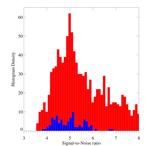
Figure 1: Histograms of S/N distribution of cataloged objects (red) and false positives (blue) eliminated via application of the CLEAN mask. The histogram range is restricted to a $S/N=8$ to emphasize the distribution of the removed false positives.

Table 1: PAWS GMC catalog

ID	RA (J2000)	Dec (J2000)	$\Delta V_{LSR}$	$T_{max}$	$S/N$	$R$	$\sigma_{v}$	$L_{CO}$	$M_{vir}$	$\alpha$	PA	b/a	Reg	Flag
	$hh\,mm\,ss.ss$	$dd\,mm\,ss.ss$	km s-1	K		pc	km s-1	$10^{5}$ K km s-1 pc2	$10^{5}$ M⊙			deg
(1)	(2)	(3)	(4)	(5)	(6)	(7)	(8)	(9)	(10)	(11)	(12)	(13)	(14)	(15)
$1$	$13^{h}30^{m}0.65^{s}$	$47^{\circ}11^{\prime}10.58"$	$-4.3$	$2.5$	$5.2$	$18\pm 19$	$3.7\pm 2.6$	$0.9\pm 0.3$	$2.7\pm 5.7$	$0.7$	$135$	$1.0$	$IA$	$0$
$2$	$13^{h}30^{m}0.87^{s}$	$47^{\circ}10^{\prime}56.15"$	$52.8$	$5.3$	$7.0$	$50\pm 8$	$10.2\pm 1.9$	$4.4\pm 0.7$	$54.0\pm 25.4$	$2.8$	$49$	$0.9$	$IA$	$0$
$3$	$13^{h}30^{m}1.54^{s}$	$47^{\circ}11^{\prime}4.84"$	$60.5$	$4.6$	$5.1$	$32\pm 0$	$10.8\pm 4.5$	$2.1\pm 0.8$	$38.5\pm 31.9$	$4.3$	$152$	$0.6$	$IA$	$1$
$4$	$13^{h}29^{m}58.01^{s}$	$47^{\circ}11^{\prime}6.34"$	$-2.4$	$1.3$	$3.8$	$32\pm 0$	$5.1\pm 3.9$	$0.7\pm 0.6$	$8.5\pm 13.0$	$2.8$	$179$	$0.2$	$SA$	$1$
$5$	$13^{h}29^{m}57.79^{s}$	$47^{\circ}11^{\prime}7.20"$	$3.3$	$2.1$	$5.8$	$40\pm 21$	$9.6\pm 3.7$	$1.6\pm 0.6$	$38.0\pm 33.7$	$5.4$	$8$	$0.9$	$SA$	$0$
$6$	$13^{h}29^{m}58.14^{s}$	$47^{\circ}11^{\prime}6.34"$	$15.3$	$2.5$	$6.7$	$27\pm 33$	$1.9\pm 2.0$	$0.6\pm 0.8$	$1.1\pm 3.2$	$0.4$	$116$	$0.6$	$SA$	$0$
$7$	$13^{h}29^{m}58.76^{s}$	$47^{\circ}11^{\prime}9.41"$	$13.4$	$2.2$	$5.8$	$32\pm 0$	$3.1\pm 3.6$	$0.3\pm 0.2$	$3.2\pm 7.6$	$2.2$	$11$	$0.4$	$SA$	$1$
$8$	$13^{h}29^{m}58.36^{s}$	$47^{\circ}11^{\prime}10.50"$	$15.8$	$2.8$	$7.8$	$32\pm 0$	$11.1\pm 7.3$	$0.5\pm 1.1$	$40.9\pm 53.3$	$18.4$	$158$	$0.5$	$SA$	$1$
$9$	$13^{h}29^{m}57.72^{s}$	$47^{\circ}11^{\prime}2.80"$	$24.0$	$4.1$	$9.9$	$118\pm 14$	$7.3\pm 1.1$	$10.8\pm 3.1$	$65.5\pm 24.8$	$1.4$	$163$	$0.5$	$SA$	$0$
$10$	$13^{h}29^{m}58.24^{s}$	$47^{\circ}11^{\prime}9.36"$	$19.6$	$5.0$	$12.0$	$32\pm 15$	$8.0\pm 3.9$	$3.8\pm 3.3$	$21.3\pm 21.6$	$1.3$	$133$	$0.6$	$SA$	$0$
…	…	…	…	…	…	…	…	…	…	…	…	…	…	…
…	…	…	…	…	…	…	…	…	…	…	…	…	…	…
…	…	…	…	…	…	…	…	…	…	…	…	…	…	…
$1507$	$13^{h}29^{m}46.33^{s}$	$47^{\circ}12^{\prime}40.28"$	$-0.4$	$2.9$	$5.6$	$32\pm 0$	$10.1\pm 3.5$	$0.9\pm 0.2$	$33.7\pm 23.4$	$9.2$	$148$	$0.6$	$IA$	$1$

Note. — (1) cloud identification number (ID), (2) Right Ascension (RA (J2000)), (3) Declination (Dec (J2000)), (4) Velocity with respect to the systematic velocity of NGC5194 ($\sim 472$ km/s, Shetty et al. 2007), (5) Peak brightness temperature ($T_{max}$), (6) Peak signal-to-noise ratio ($S/N$), (7) Radius (R), (8) Velocity dispersion ($\sigma_{v}$), (9) CO luminosity ($L_{CO}$), (10) Mass from virial theorem ($M_{vir}$), (11) Virial parameter ($\alpha$), (12) Position angle of cloud major axis, measured from North through West (PA), (13) Ratio between minor axis and major axis ($b/a$), (14) Region of M51 where a given cloud has been identified, i.e. center (CR), spiral arms (SA), inter-arm (IA), (15) Flag$=0$ indicates the default measurement of the cloud radius, Flag$=1$ indicates that the radius is substituted with an upper limit.

5 Environmental dependence of the GMC properties in M51

Previous observations of M51 have indicated that galactic environment is important for the organization and properties of the molecular gas. Recently, for example, Koda et al. (2009) showed that M51’s spiral arms contain giant molecular associations (GMAs) with masses between $10^{7}-10^{8}$ M_⊙, while the inter-arm region hosts only smaller clouds with masses less than $\sim 10^{6}$ M_⊙. To test whether the physical properties of GMCs depend on environment in M51, we divide the PAWS FoV into seven distinct regions (see Section 5.1). We analyze the global properties of the CO emission and the GMC ensemble in Section 5.2. Environmental trends in the GMC property distributions are examined in Section 5.3.

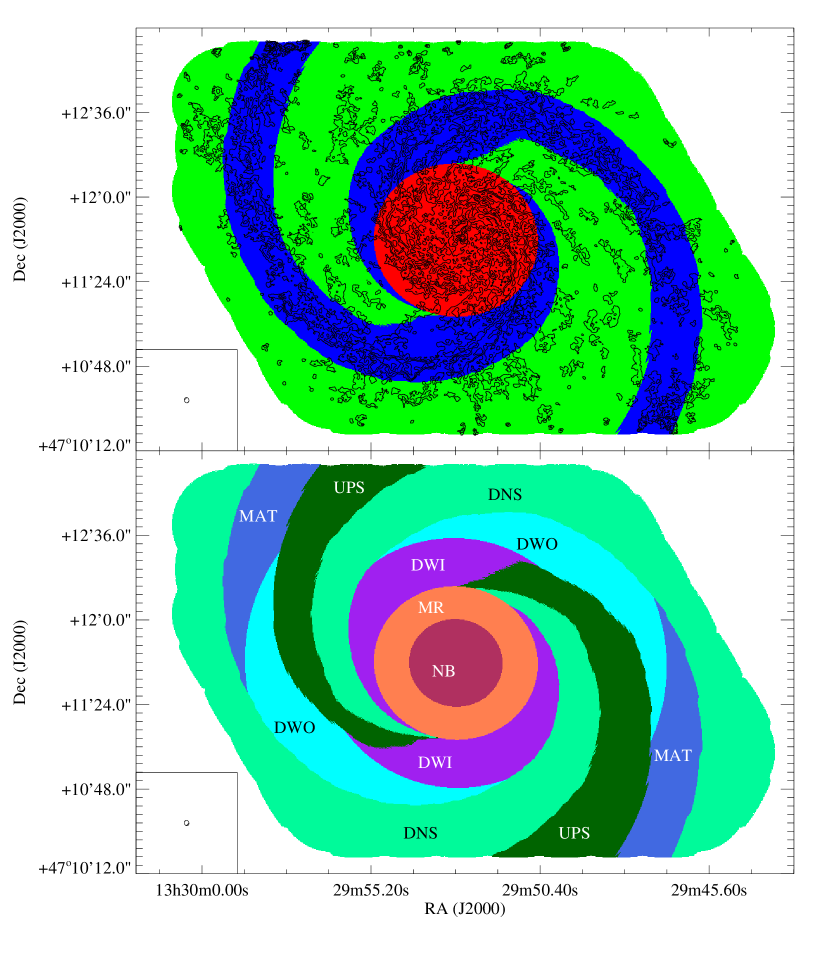
Figure 2: Top: the three main regions in which the PAWS field of view is divided: center in red, spiral arm in blue and inter-arm in green. Contours at 10, 50, 100, 200 and 400 K km s^-1 belong to the integrated intensity map of islands. Bottom: M51 environmental mask. Nuclear bar (NB) and molecular ring (MR) are indicated in dark red and orange, respectively. Inner density-wave spiral arms (DWI) are indicated in purple, outer density-wave spiral arms (DWO) in cyan, and material arms (MAT) in light blue. Downstream with respect to the spiral arms (DNS) is shaded light green while upstream is shaded dark green (UPS). These color codes will be kept throughout the paper. In the bottom left of both panels the beam ($\sim 1"$ or 40 pc) is shown.

5.1 M51 environment definition

We use the stellar potential of M51 to divide the PAWS FoV into seven distinct dynamical environments, each of which contains a statistically significant GMC population. Initially, we distinguish between the “center” ($R_{gal}\lesssim 1.3$ kpc) and “disk” ($1.3\lesssim R_{gal}\lesssim 5$ kpc) regions within the PAWS FoV. The central region (CR) is further separated into i) a nuclear bar (NB) region that is located within the corotation resonance of the bar, and ii) the molecular ring (MR), which is a zone of zero torque created by the combined dynamical effects of the spiral and nuclear bar. The “disk” region is divided azimuthally into spiral arm (SA) and inter-arm (IA) zones. Based on the direction of the gas flow within the arms derived from the torque map (Meidt et al. 2013) and tracers of massive star formation activity, we segment the spiral arm region radially into: i) inner density-wave spiral arms (DWI), ii) outer density-wave spiral arms (DWO) and iii) material arms (MAT). We divide the inter-arm zones into downstream (DNS) and upstream (UPS) regions relative to the spiral arms. The seven environments within the PAWS FoV are illustrated in Fig. 2. We describe the construction of our environmental mask in more detail in Appendix C.

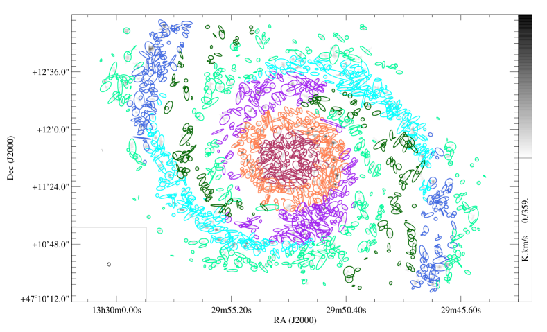
Figure 3: The GMC distribution in the PAWS field of M51 superimposed on the integrated identified object CO intensity map (grey-scale). The sidebar indicates the color scale of the map in K km s^-1. The GMCs are represented as ellipses with the extrapolated and deconvolved major and minor axes, oriented according to the measured position angle. The clouds that appear overlapping are actually separated along the velocity axis. Colors indicate the environment in which a given object has been identified following the color code of Fig. 2. These color codes will be kept throughout the paper. In the bottom left of both panels the beam ($\sim 1"$ or 40 pc) is shown.

5.2 Properties of CO emission and the GMC Ensemble in Different M51 Environments

In Table 2, we list several key properties of the CO emission and GMC populations within the different galactic environments. These tabulated properties include the total CO luminosity, the fraction of the CO emission that is relatively bright and hence included within the CPROPS “working area”, and the total number and number density of GMCs. One obvious difference between the environments is the contribution of high S/N emission to the region’s total CO luminosity: emission belonging to the CPROPS working area constitutes 80-90% of the CO luminosity present in the spiral arm and central regions, but only $\sim 45\%$ of the inter-arm emission. Another way to quantify this is via the average H₂ mass surface density ($\Sigma_{H_{2}}$) calculated across each region. Assuming a constant conversion factor ($X_{CO}=2\times 10^{20}$cm^-2 (K km s^-1)^-1), the center of M51 has the highest H₂ mass surface density $\Sigma_{H_{2}}=237$ M_⊙ pc^-2, while in the spiral arm and in the inter-arm regions the $\Sigma_{H_{2}}$ is a factor 2 and 6 lower, respectively. Since the area of the inter-arm relative to the spiral arm increases with galactocentric radius, this decline is consistent with the radial decrease in the molecular mass surface density reported by lower resolution CO studies of M51, e.g. Schuster et al. (2007). The number density of clouds, $N_{GMC}$, shows a similar trend as $\Sigma_{H_{2}}$, decreasing from 72 kpc^-2 in the central region to 45 kpc^-2 in the spiral arms and 19 kpc^-2 in the inter-arm region.

Table 2 shows that the flux associated with GMCs ($L_{CO}^{EX}$) is 54% of the total flux in the PAWS data cube $L_{CO}\approx 91\times 10^{7}$ K km s^-1 pc² . A significant fraction of the emission of the PAWS cube is thus not decomposed by CPROPS into GMCs. The remaining flux could be due to structures smaller than the beam or in the extended component identified by Pety et al. (2013). We note that the CO luminosity contained in the identified objects ($L_{CO}^{NX}$) is only $\sim 20\%$ of the total flux in the cube, i.e. more than half of the combined flux of GMCs is recovered through the extrapolation step of the CPROPS decomposition algorithm. We discuss this issue further in Section 5.4.

Table 2: Global Properties of M51’s GMC population and environments

Envir.	Whole region			Working Area		GMC
	(1)A	${}^{(2)}L_{CO}$	${}^{(3)}\Sigma_{H_{2}}$	(4)A	${}^{(5)}L_{CO}$	${}^{(6)}L_{CO}^{NX}$	${}^{(7)}L_{CO}^{EX}$	${}^{(8)}\%^{NX}$	${}^{(9)}\%^{EX}$	(10)#	(11)NGMC
	[kpc2]	[$10^{7}$ K km s-1 pc2]	[M⊙ pc${}^{-2}]$	[kpc2]	[$10^{7}$ K km s-1 pc2]	[$10^{7}$ K km s-1 pc2]					[kpc-2]
Cube	47.0	90.83	84.22	11.5	67.08	17.81	48.65	20	54	1507	32
CR	4.7	25.47	237.02	1.2	22.85	4.71	14.48	18	57	335	73
SA	14.6	43.44	129.94	2.3	35.10	8.16	23.22	21	59	657	45
IA	27.8	21.88	34.37	1.0	9.12	4.93	10.93	19	42	514	19
NB	1.5	7.48	213.11	2.7	6.49	1.43	4.18	19	56	126	82
NR	3.2	17.99	248.62	5.5	16.35	3.28	10.30	18	57	209	66
DWI	4.2	5.50	56.90	3.3	4.75	2.32	7.23	18	55	204	48
DWO	5.3	10.54	87.09	1.0	9.16	3.69	10.72	20	58	274	52
MAT	3.9	3.50	39.31	1.7	2.33	2.15	5.27	27	65	179	46
DNS	20.7	8.21	17.25	1.8	6.81	3.57	7.66	20	43	350	17
UPS	8.2	10.13	53.70	2.5	8.25	1.36	3.27	17	42	164	20

Note. — ⁽¹⁾ area encompassed by M51’s environments; ⁽²⁾ CO luminosity contained in the environment area; ⁽³⁾ H₂ mass surface density of the given environment; ⁽⁴⁾ area encompassed by M51’s environment working areas; ⁽⁵⁾ CO luminosity contained in the environment area within the working area; ⁽⁶⁾ and ⁽⁷⁾ CO luminosity associated with identified GMCs, before and after extrapolation, respectively; ⁽⁸⁾ and ⁽⁹⁾ percentage CO luminosity contained in GMCs, before and after extrapolation, respectively, with respect to the total CO luminosity of the environment; ⁽¹⁰⁾ number of GMCs in a given environment; ⁽¹¹⁾ number density of GMCs in a given environment.

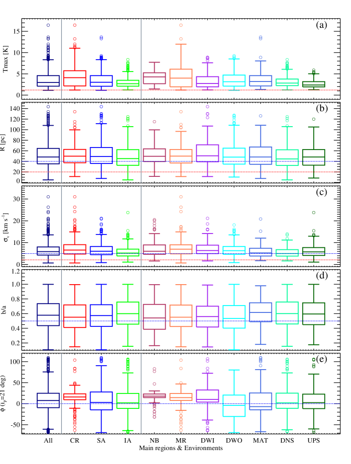
Figure 4: Basic GMC properties (from the top to the bottom): (a) peak brightness temperature $T_{max}$, (b) effective radius $R$, (c) velocity dispersion $\sigma_{v}$, (d) axis ratio $b/a$ and (e) orientation $\phi$ shown in a “box and whiskers” representation for different M51 environments (from the left to the right: All -full sample; 3 main regions -center (CR), spiral arm (SA), inter-arm (IA) and 7 environments defined in Fig. 2 and Appendix C). The box middle band represents the median of the distribution. The box itself contains $50\%$ of the data points. Each whisker that emerges from the box, coinciding with $\sim 25\%$ of the data points, corresponds roughly to $3\sigma$ of a normal distribution. The median of velocity dispersion and brightness temperature is always higher in the central region (CR and MR, NB) and in the density-wave spiral arms (DWI and DWO), compared to inter-arm environments (DNS, UPS). Straight horizontal red lines indicate the resolution, instrumental or sensitivity limits: 1.2 K for the peak brightness temperature, 20 pc for the radius, 2.12 km s^-1 for the velocity dispersion. Reference lines at arbitrary values are indicated in blue to help guide the eye. Circles represent the outliers of the distribution (see description at the beginning of Section 5.2).

5.3 Variation of GMC physical properties with environment

In this section, we examine whether the physical properties of GMCs – such as radius, velocity dispersion and mass – vary with galactic environment. To visualize the GMC property distributions, we use a “box and whiskers” plot (e.g. Tukey 1977) in Figures 4 and 5. This representation is a useful tool to identify and illustrate differences in the shape of non-Gaussian distributions. The box is delimited by two lines that indicate the lower $Q25$ and upper $Q75$ quartiles of the distribution. The middle band represents the median. For a normal distribution, the interquartile range or distribution spread ($IQR\equiv Q75-Q25$) corresponds to $1.35\sigma$, where $\sigma$ is the standard deviation. $0.5IQR$ corresponds to $0.6745\sigma$ or to the median absolute deviation (MAD). The ends of the whiskers indicate the lowest and the highest data points that lie within 1.5 $\times IQR$ of the lower quartile (the bottom whisker, BW) and 1.5 $\times IQR$ of the upper quartile (the top whisker, TW). For a normal distribution, the range of values between TW (or BW) and the middle band roughly corresponds to $\pm 3\sigma$. We define “outliers” as data points with values lower or greater than BW or TW, respectively (i.e. outside the $3\sigma$ range of a Gaussian distribution), and represent them as circles in the box and whiskers plots. The median and the lower and upper quartiles ($Q25$ and $Q75$, respectively) of the GMC property distributions are listed in Table 3.

To test the statistical significance of differences between the GMC property distributions, we use the two-sided Kolmogorov-Smirnov (KS) test (e.g. Eadie et al. 1971) on both the full and the “highly reliable cloud” samples. The two-sided KS statistic quantifies a distance between the empirical distribution functions of two samples assuming as a null hypothesis that the samples are drawn from the same parent distribution. This distance is directly connected to the p-value, the probability that two samples descend from the same parent population. Traditionally, the null hypothesis is rejected when the p-value is smaller than a certain significance level. We adopt the convention that there is a significant difference between two samples if the p-value is lower than 0.001, while p-values less than or equal to 0.05 indicate marginally significant differences. We use a modified version of the two-sided KS test that attempts to account for measurement uncertainties (for details see Appendix D).

Table 3: GMC properties in the different environments of M51

	GMC Property
Env.	Basic					Derived
	$T_{max}$	R	$\sigma_{v}$	b/a	$\phi$	$M_{lum}$	$M_{vir}$	$\Sigma_{H_{2}}$	$c$	$\alpha$
	[K]	[pc]	[km s-1]		[deg]	[$10^{5}$ M⊙]	[$10^{5}$ M⊙]	[M⊙ pc-2]	[km s-1 pc-1/2]
All	$3.0^{+4.6}_{-2.1}$	$48.4^{+64.5}_{-35.4}$	$5.9^{+8.0}_{-4.3}$	$0.6^{+0.7}_{-0.4}$	$7.6^{+24.8}_{-9.4}$	$7.6^{+16.5}_{-3.4}$	$19.6^{+40.5}_{-9.4}$	$177.4^{+298.5}_{-110.2}$	$0.9^{+1.3}_{-0.7}$	$1.6^{+3.2}_{-0.9}$
CR	$4.1^{+5.7}_{-2.2}$	$49.8^{+62.7}_{-37.4}$	$6.6^{+9.1}_{-4.8}$	$0.6^{+0.7}_{-0.4}$	$15.9^{+23.5}_{-9.4}$	$10.4^{+24.0}_{-3.9}$	$25.1^{+50.2}_{-12.5}$	$212.4^{+368.2}_{-129.2}$	$1.0^{+1.4}_{-0.7}$	$1.5^{+3.5}_{-0.9}$
SA	$3.0^{+4.6}_{-2.1}$	$49.3^{+66.3}_{-36.0}$	$6.1^{+8.2}_{-4.5}$	$0.6^{+0.7}_{-0.4}$	$2.9^{+27.9}_{-14.6}$	$8.3^{+18.2}_{-3.6}$	$21.7^{+45.1}_{-10.7}$	$185.3^{+304.1}_{-112.4}$	$1.0^{+1.3}_{-0.7}$	$1.7^{+3.0}_{-0.9}$
IA	$2.7^{+3.5}_{-2.1}$	$45.3^{+62.2}_{-32.6}$	$5.2^{+7.0}_{-3.9}$	$0.6^{+0.8}_{-0.5}$	$2.1^{+24.3}_{-11.3}$	$5.8^{+11.0}_{-3.1}$	$14.8^{+31.0}_{-6.9}$	$143.4^{+228.1}_{-94.0}$	$0.8^{+1.2}_{-0.6}$	$1.6^{+3.2}_{-0.8}$
NB	$4.3^{+5.2}_{-2.7}$	$49.6^{+63.8}_{-39.6}$	$6.1^{+9.0}_{-4.6}$	$0.5^{+0.7}_{-0.4}$	$17.9^{+23.0}_{-14.5}$	$10.7^{+19.8}_{-5.7}$	$20.7^{+49.8}_{-11.5}$	$184.3^{+291.1}_{-111.6}$	$0.9^{+1.3}_{-0.6}$	$1.5^{+3.7}_{-0.9}$
MR	$4.0^{+6.1}_{-2.0}$	$50.0^{+62.4}_{-36.9}$	$7.0^{+9.0}_{-4.9}$	$0.6^{+0.7}_{-0.4}$	$14.4^{+24.1}_{-7.7}$	$10.4^{+27.1}_{-3.5}$	$26.8^{+50.2}_{-13.6}$	$227.4^{+387.6}_{-141.8}$	$1.0^{+1.4}_{-0.8}$	$1.6^{+3.4}_{-0.9}$
DWI	$2.7^{+4.3}_{-1.9}$	$50.5^{+71.3}_{-39.3}$	$6.4^{+8.8}_{-5.0}$	$0.6^{+0.7}_{-0.4}$	$10.1^{+32.6}_{-3.8}$	$8.5^{+16.5}_{-3.7}$	$29.9^{+52.0}_{-12.6}$	$155.0^{+251.9}_{-110.2}$	$1.0^{+1.3}_{-0.7}$	$2.1^{+3.6}_{-1.2}$
DWO	$3.2^{+4.7}_{-2.1}$	$48.1^{+65.0}_{-34.8}$	$6.3^{+8.2}_{-4.6}$	$0.5^{+0.7}_{-0.4}$	$-4.2^{+20.5}_{-30.4}$	$8.6^{+22.8}_{-3.8}$	$22.8^{+42.3}_{-11.4}$	$218.7^{+317.3}_{-123.5}$	$1.0^{+1.3}_{-0.8}$	$1.7^{+2.7}_{-1.0}$
MAT	$3.2^{+4.6}_{-2.2}$	$48.3^{+67.2}_{-34.5}$	$5.3^{+7.4}_{-3.9}$	$0.6^{+0.7}_{-0.5}$	$-7.0^{+25.5}_{-14.5}$	$7.1^{+15.0}_{-3.1}$	$15.0^{+31.6}_{-8.7}$	$180.1^{+319.3}_{-92.3}$	$0.8^{+1.3}_{-0.6}$	$1.5^{+2.5}_{-0.8}$
DNS	$2.8^{+3.8}_{-2.2}$	$44.7^{+62.0}_{-32.3}$	$5.0^{+6.8}_{-3.9}$	$0.6^{+0.8}_{-0.5}$	$2.1^{+25.0}_{-10.9}$	$5.9^{+11.9}_{-3.1}$	$12.8^{+27.7}_{-6.7}$	$147.0^{+235.0}_{-94.5}$	$0.8^{+1.1}_{-0.6}$	$1.5^{+2.5}_{-0.8}$
UPS	$2.4^{+3.2}_{-1.9}$	$48.3^{+62.3}_{-32.8}$	$5.8^{+7.7}_{-4.1}$	$0.6^{+0.7}_{-0.5}$	$2.5^{+22.7}_{-11.7}$	$5.3^{+10.3}_{-3.1}$	$17.7^{+37.4}_{-7.5}$	$139.1^{+215.9}_{-92.5}$	$0.9^{+1.3}_{-0.6}$	$1.9^{+4.3}_{-0.8}$

Note. — Median, lower quartile ($Q25$) and upper quartile ($Q75$) of the distributions. For Gaussian distributions a quartile corresponds to $0.6745\sigma$ or to the median absolute deviation (MAD).

5.3.1 Basic GMC properties

In Fig. 4, we plot the distribution of basic GMC properties within each of our environments. The results of the KS tests that were used to assess whether the distributions exhibit significant differences are reported in Appendix D. Fig. 4a and Fig. 4c show that the distributions of GMC peak brightness temperature T_max and velocity dispersion $\sigma_{v}$ exhibit the most significant environmental variations: both properties tend to decrease from the center to the spiral arm to the inter-arm region. In the spiral arms and central region, GMCs span a large range of T_max and $\sigma_{v}$ values, while the inter-arm region lacks GMCs with high T_max and $\sigma_{v}$. There is also a subtle difference between the peak brightness of inter-arm GMCs, such that upstream GMCs tend to have lower T_max than downstream clouds. The KS tests generally confirm these findings.

Galactic environment appears to have at most a modest impact on the size and elongation of GMCs in M51 (Fig. 4b and Fig 4d). GMCs in M51 are generally elongated with an axis ratio $b/a$ around $\sim 0.6$. However, clouds in the material arm and inter-arm regions have a slightly higher $b/a$ and visually appear more round. By contrast, the cloud orientation, $\phi$, shows a clear connection to galactic structure in M51. Fig. 4e shows that $\langle\phi\rangle$ is generally close to $0^{\circ}$ in the spiral arm and inter-arm regions, confirming that the GMC orientation follows the spiral geometry. Clouds in the central region show a larger deviation from the spiral arm model, which is expected since the molecular ring is not a direct extension of the spiral arms. Nevertheless, the width of the $\phi$ distributions in all environments is fairly large. One possible explanation is that the CO spiral arms are not perfect logarithmic spirals. Although they are well-approximated by a double logarithmic spiral with $i_{p}=21^{\circ}\pm 5^{\circ}$ for galactocentric radii $1.9<R_{gal}<5.5$ kpc (Patrikeev et al. 2006) several breaks are evident in a polar representation (see. Fig. 3 in Schinnerer et al. 2013). Another source of scatter might be due to GMCs located in the spurs that are orthogonal to the spiral arms (especially evident along the northern arm, see Figure 3).

5.3.2 Derived GMC properties

In Figure 5, we plot the distributions of GMC mass, as inferred from both the CO luminosity and the virial theorem, H₂ mass surface density, scaling coefficient and virial parameter for each of the M51 environments. The differences in the brightness and velocity dispersion of GMCs that we detected in Fig. 4 are likely to produce variations in the distributions of cloud properties that are estimated using a combination of these parameters. This is what we observe: Fig. 5a shows the GMC mass inferred from the CO luminosity $M_{lum}$ declines from the central and density-wave spiral arm regions to the material arm and inter-arm regions. This is expected since $M_{lum}\propto L_{CO}\propto\langle T\rangle R^{2}\sigma_{v}$. In broad terms, the mass derived from the virial theorem exhibits a similar trend (see Fig. 5b), although by definition it is dependent only on $\sigma_{v}$ and $R$. We note that the average virial mass for GMCs in the PAWS catalog is $\sim 2\times$ greater than the average value of $M_{lum}$, derived assuming $X_{CO}=2\times 10^{20}$cm^-2 (K km s^-1)^-1.

Fig. 5c shows that the average GMC mass surface density $\langle\Sigma_{H_{2}}\rangle$ is highest in the central zone (212 M_⊙ pc^-2), and lower in spiral arm (185 M_⊙ pc^-2) and the inter-arm region (143 M_⊙ pc^-2). Across the entire PAWS FoV, the median H₂ mass surface density is $\Sigma_{H_{2}}\approx 180$ M_⊙ pc^-2, almost twice the average value observed for GMCs in the inner Milky Way ($\sim 100$ M_⊙ pc^-2, Heyer et al. 2009). We note that the PAWS and Galactic values are not strictly comparable: the Galactic structures described by Heyer et al. (2009) are typically smaller than the GMCs in M51, and are observed at high spatial resolution (i.e. the telescope beam is much smaller than the angular size of the observed GMCs). The filling factor of CO emission within the PAWS beam, by contrast, is likely to be less than unity since the typical peak brightness is only T${}_{max}\approx 4$ K. The difference between the typical mass surface densities of the M51 and Milky Way GMCs is therefore probably a lower limit, with high resolution observations likely to yield even higher mass surface densities for M51 cloud structures.

Fig. 5e shows that the median value of the virial parameter is $\sim 1.6$ across all M51 environments, with values for individual GMCs ranging between 1 and 8. This suggests that the GMC population in M51 is, on average, self-gravitating, although $\sim 30$% of the clouds have $\alpha>2$. The fraction of clouds with $\alpha>2$ is higher for the upstream subsample than for the downstream subsample of GMCs. Fig. 5d shows that the average scaling coefficient $c=0.90$ km s^-1 pc^-1/2 of the size-linewidth relation is also roughly constant across the different environments. The median value $\langle c\rangle\approx 0.90$ km s^-1 pc^-1/2 is always higher than the Galactic value of $0.72$ km s^-1 pc^-1/2 (S87), indicating that GMCs in M51 tend to have higher velocity dispersions than GMCs with comparable size in the Milky Way.

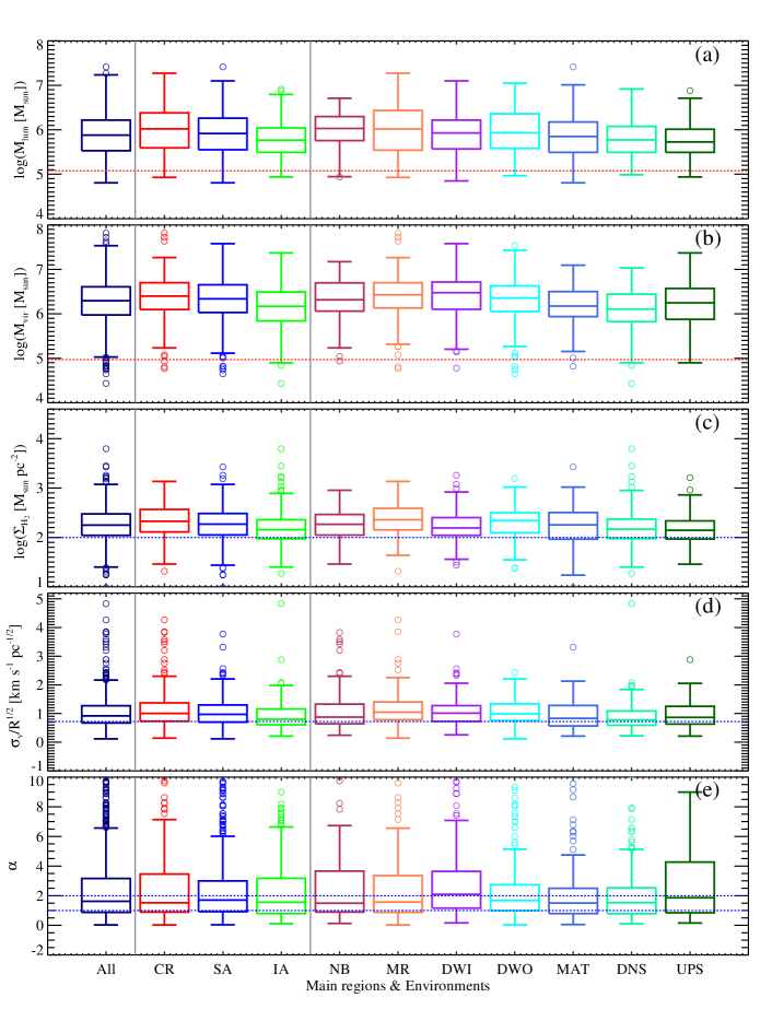
Figure 5: Derived GMC properties (from top to bottom): (a) mass derived from CO luminosity $M_{lum}$ and (b) using the virial theorem $M_{vir}$, (c) H₂ surface density $\Sigma_{H_{2}}$, (d) scaling coefficient $\sigma_{v}/R^{1/2}$ and (e) virial parameter $\alpha$ shown in a “box and whiskers” representation (see Fig. 4 for details) for different M51 environments (from the left to the right: All -full sample; 3 main regions -center (CR), spiral arm (SA), inter-arm (IA) and the 7 environments defined in Fig. 2 and Appendix C). In general masses, H₂ mass surface densities and scaling coefficients are higher in the center and in the spiral arm region than in the inter-arm environments. The cloud population in every environment is, in general, self-gravitating, however a number of objects appears unbound ($\alpha>2$). Straight horizontal red lines indicate the sensitivity or resolution limits: $1.2\times 10^{5}$ $M_{\odot}$ for the luminosity mass and $10^{5}$ $M_{\odot}$ for the virial mass. For surface density and scaling coefficient the blue lines show values observed in the Galaxy: $100$ M_⊙ pc^-2 (Heyer et al. 2009) and $0.72$ km s^-1 pc^-1/2 (S87), respectively. Horizontal blue lines in the virial parameter panel indicate the limit for the virialized ($\alpha=1$) and self-gravitating objects ($\alpha=2$) (see text for details).

5.3.3 Radial Trends in GMC Properties

Our investigation differs from several previous surveys of molecular gas across the disk of external galaxies, which have tended to analyze the properties of the molecular gas and/or GMCs as a function of galactocentric radius (e.g. Hitschfeld et al. 2009, Gratier et al. 2012). In contrast to these CO surveys, PAWS is restricted to the inner disk of M51 ($R_{gal}\lesssim 5$ kpc), and many environmental parameters that could produce a change in the GMC properties show only modest variations. For example, the molecular gas fraction $M_{H_{2}}/(M_{H_{2}}+M_{H})$ is $\sim 80$% across the FoV (Leroy et al. 2008, but see also Schuster et al. 2007, Koda et al. 2009), while the dust-to-gas ratio and ambient interstellar radiation field are roughly constant across our FoV (Mentuch Cooper et al. 2012, Muñoz-Mateos et al. 2011).

Nevertheless, for comparison with previous studies, we examined whether the GMC properties exhibit trends with galactocentric radius. We divided the PAWS FoV into 5 radial bins (2 covering the central region, 3 for the disk) of $\sim 2$ kpc width, each containing $\sim 300$ objects, and compared the statistics of the cloud property distributions in the different radial bins. As seen in Fig. 4 and 5, clouds in the central region tend to have higher peak brightness temperatures, velocity dispersions and CO luminosities compared to clouds at larger radii. Within the bins covering the disk region, however, we see no evidence for variations in the average physical properties of the GMCs with galactocentric radius. Due to the shape of the PAWS FoV, each radial disk bin contains an almost equal number of spiral arm and inter-arm GMCs. We conclude that this uniform mixture of arm and inter-arm clouds suppresses the environmental variations that we described above when we examine the cloud properties as a function of galactocentric radius beyond the central zone. In light of our results for the GMCs in PAWS, it would be interesting to examine whether the radial trends reported by previous studies reflect a combination of variations between the properties of clouds in the arm and inter-arm regions, as well as variations along the spiral arms.

Table 4: Median of corrections applied to measurements of GMC properties

Envir.	Sensitivity			Resolution		Global
	$R^{ext}/R^{obs}$	$\sigma_{v}^{ext}/\sigma_{v}^{obs}$	$L_{CO}^{ext}/L_{CO}^{obs}$	$R^{dec}/R^{obs}$	$\sigma_{v}^{dec}/\sigma_{v}^{obs}$	$R^{corr}/R^{obs}$	$\sigma_{v}^{corr}/\sigma_{v}^{obs}$
All	1.6	1.6	2.5	0.7	0.8	1.3	1.5
CR	1.8	1.8	2.8	0.7	0.8	1.5	1.7
SA	1.6	1.7	2.6	0.7	0.9	1.3	1.6
IA	1.4	1.4	2.1	0.7	0.8	1.1	1.3
NB	1.8	1.8	2.8	0.7	0.8	1.5	1.7
MR	1.6	1.6	2.5	0.7	0.9	1.4	1.5
DWI	1.6	1.6	2.5	0.7	0.8	1.2	1.5
DWO	1.4	1.4	2.2	0.7	0.8	1.2	1.4
MAT	1.5	1.4	2.2	0.7	0.8	1.2	1.3
DNS	1.8	1.8	2.8	0.7	0.8	1.5	1.7
UPS	1.6	1.6	2.5	0.7	0.9	1.4	1.5

Note. — Median of the sensitivity, resolution and global corrections applied to the observed values of the GMC properties as a function of environment.

5.4 The effect of CPROPS bias corrections on GMC property measurements

As noted in Section 5.2, the flux contained in the cataloged GMCs is nearly three times greater than the flux that is directly measured within the objects that are initially identified by CPROPS. Here, we assess the reliability of the cloud property measurements in our catalog, paying particular attention to whether the environmental trends that we described above could result from the CPROPS extrapolation and deconvolution corrections.

5.4.1 Dependence of resolution and sensitivity correction on environment

In Table 4, we list the median ratio of the corrected and uncorrected cloud properties within the different M51 environments. The properties related to the identified objects are indicated with the superscript obs, the superscript ext denotes the extrapolated (but not deconvolved) GMC properties, while dec stands for deconvolution from the beam or the channel width (without extrapolation). The superscript corr denotes cloud properties corrected for both resolution and sensitivity bias, and corresponds to the cloud property values listed in the catalog.

The resolution correction (i.e. deconvolution for beam or channel width) is approximately constant with environment, decreasing the effective radius and velocity dispersion of GMCs across the PAWS FoV by 20-30% on average. The sensitivity correction (i.e. extrapolation), by contrast, varies with environment. Compared to the extrapolated radius $R^{ext}$, the observed radius $R^{obs}$ is underestimated by $\sim 80\%$ in the central region, $\sim 60\%$ in the spiral arms and $\sim 40\%$ in the inter-arm region. The sensitivity correction yields a similar trend for the velocity dispersion measurements. The CO luminosity is even more dependent on extrapolation than the radius and velocity dispersion measurements: $L_{CO}^{ext}$ is typically a factor of $\sim 1.5$ to 2 higher than its uncorrected value for clouds in the central and spiral arm regions, and a factor of $\sim 1.3$ higher in the inter-arm region.

The combined effect of the CPROPS corrections on the cloud radius and velocity dispersion is summarized in the final two columns of Table 4 and illustrated in Fig. 6. The correction is higher in the central region and in the density-wave spiral arm where $R^{corr}$ is around $30-50\%$ higher than $R^{obs}$. In the inter-arm region, the corrected radius is only $\sim 10\%$ higher than the uncorrected one. The CPROPS corrections have a larger impact on the velocity dispersion: in the central and spiral arm regions, the corrected $\sigma^{corr}_{v}$ is $60-70\%$ higher than the uncorrected measurement. In the inter-arm region, $\sigma^{corr}_{v}$ is $\sim 40\%$ higher than the uncorrected velocity dispersion.

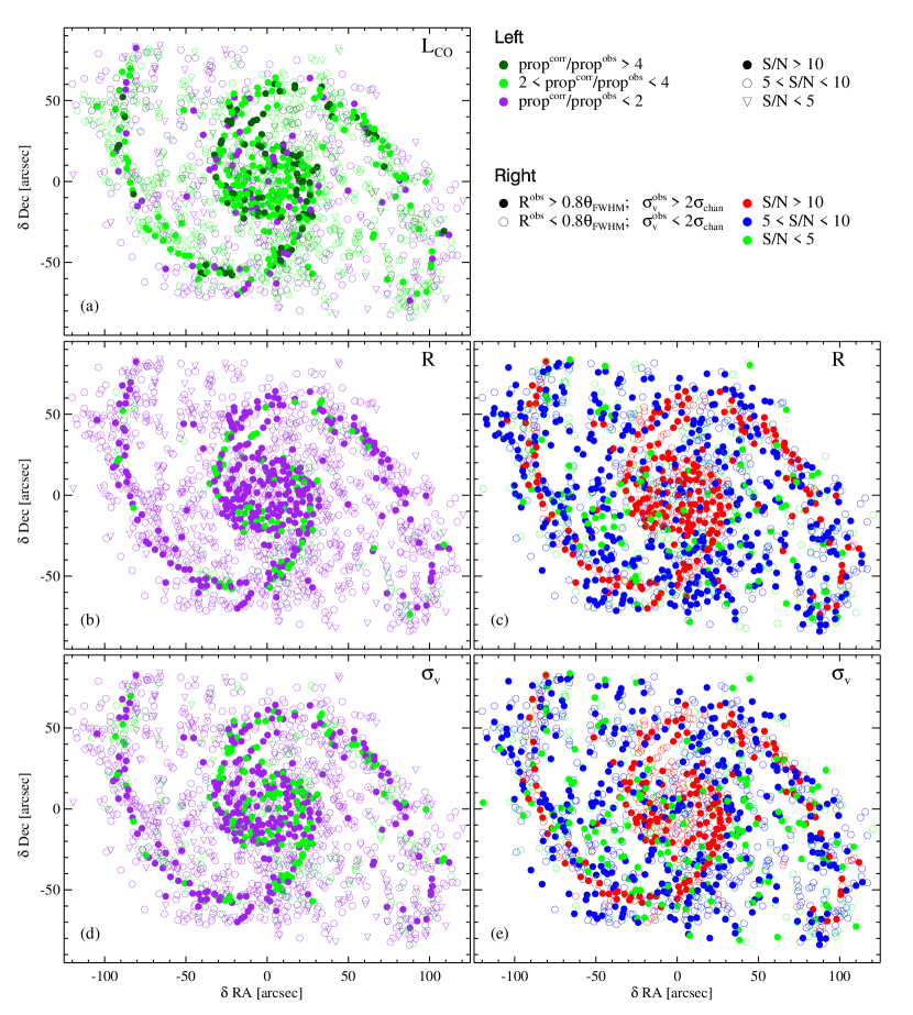
Figure 6: Left: Spatial illustration of the global correction applied to (a) the CO luminosity, (b) effective radius and (d) velocity dispersion measurements of GMCs as a function of signal-to-noise ($S/N$). The superscript corr refers to GMC properties corrected for both sensitivity and resolution biases, while the superscript obs to the properties of identified objects. Right: Spatial illustration of the reliability of (c) the effective radius and (e) velocity dispersion measurement as a function of $S/N$. A cloud is considered fully resolved by CPROPS if $R^{obs}>0.8\theta_{FWHM}$ and $\sigma_{v}^{obs}>2\sigma_{v}^{chan}$, where $R^{obs}$ and $\sigma_{v}^{obs}$ represent the effective radius and the velocity dispersion of the identified objects, respectively; while $\theta_{FWHM}$ and $\sigma_{v}^{chan}$ are the beam FWHM and the channel width. Axis coordinates refer to the galactic center 13h 29m 52.7087s ;+47^∘ 11′ 42.789” (Hagiwara 2007).

The environmental dependence of the sensitivity correction becomes easy to understand if we consider the method that CPROPS uses to perform the extrapolation. An identified object is defined as a set of (x,y,v) pixels with brightness temperature $T>T_{edge}^{min}$, where $T_{edge}^{min}$ represents the cloud boundary above a certain signal-to-noise level. The unextrapolated properties derived for the identified objects are then a function of the cloud boundary, whereas the estimate of the properties at $T\equiv 0$ K (extrapolation for perfect sensitivity) is performed using a weighted linear – or, for the flux, quadratic – least-squares fit that takes into account the brightness temperature profile within the cloud. Thus the difference between the cloud property values before and after the sensitivity correction (extrapolation) is determined by the magnitude of the brightness temperature gradient within the cloud and consequently by the value of $T_{edge}^{min}$.

To test whether the cloud brightness temperature gradient varies with environment, we analyzed the full cloud sample in the three main regions (i.e. M51’s center, spiral arms, and inter-arm). We fixed 10 $T_{edge}$ levels corresponding to $10\%-20\%-...100\%$ of the peak temperature of a cloud and we calculated the radius, the CO luminosity and CO surface brightness of the object at each level. The radius is estimated as:

$$R=\sqrt{\frac{A}{\pi}},$$ (13)

where $A$ is the area of the cloud (in pixels) at a given $T_{edge}$. Figure 7 shows the result as a median of the property distribution at a given $T_{edge}/T_{max}$ value. The cloud radius profiles show similar slopes in all three environments. The CO luminosity profiles, however, appear steeper in the central region. The surface brightness profiles $I_{CO}$ also differ between the three main regions. The central region profile is the steepest, and the inter-arm profile is the most shallow. These differences indicate that the brightness temperature gradient inside the clouds is varying between the different regions, which explains why the magnitude of the sensitivity correction depends on environment.

The difference between the extrapolated and uncorrected properties is also proportional to the value of $T_{edge}^{min}$. We can assess the effect of $T_{edge}^{min}$ by examining the brightness temperature distributions of the watershed (i.e. undecomposed emission within the CPROPS working area) in the different environments. In the central and spiral arm regions, where the difference between extrapolated and unextrapolated properties is higher, large areas have brightness temperatures $>4$ K. In the inter-arm region, where the difference between corrected and uncorrected properties is lower, the watershed mostly has brightness temperatures $<2$ K.

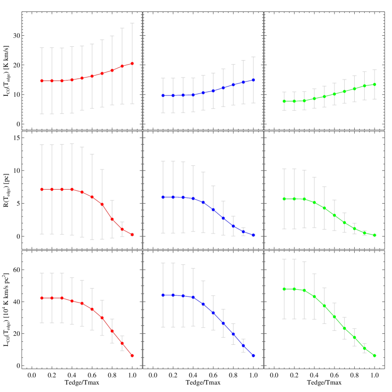
Figure 7: Median of cloud profiles relative to surface brightness $I_{CO}$ (top), effective radius $R$ (middle), and CO luminosity $L_{CO}$ (bottom) for the three main region (from left to right: central, spiral arm and inter-arm region). Error bars indicate the median absolute deviation of the distributions.

5.4.2 Reliability of extrapolated property measurements

CPROPS obtains measurements of GMC properties only if certain requirements on the sensitivity and resolution are satisfied (RL06). Here we take a conservative approach, examining the properties of the identified objects in order to determine whether the final corrected measurements can be considered reliable.

As discussed by RL06, the sensitivity correction of CPROPS will yield the effective radius of a cloud with an error below $10\%$ if the signal-to-noise $S/N$ is greater than 10. The algorithm performs well even for barely resolved objects, i.e. for clouds with $R^{obs}>0.8\theta_{FWHM}$, where $\theta_{FWHM}$ is the full width at half maximum size of the beam. For clouds with $5<S/N<10$, the measured radius may be underestimated by up to $20\%$. The accuracy of the corrected radius measurements deteriorates for faint clouds ($S/N<5$), and when an object is unresolved.

Fig. 6 shows the spatial distribution of M51 clouds as a function of the signal-to-noise and the observed radius relative to the beam size. The identified clouds with $S/N>10$ constitute $\sim 25\%$ of the catalog. These clouds are typically located in the ridge line of the spiral arms and in the central region. More than $50\%$ of the objects have a $S/N$ between 5 and 10 and the remaining $25\%$ of clouds have $S/N<5$. These faint clouds are distributed across the PAWS field. The objects with a peak signal-to-noise above 5 that satisfy the resolution requirement of CPROPS ($R^{obs}>0.8\theta_{FWHM}$) are $40\%$ of the total, while the objects with an observed radius below this limit that show the same range of $S/N$ are more than $\sim 35\%$ of the catalog and could suffer a 10% underestimation of their actual radii. Thus $65\%$ of the clouds have a radius measurement that can be considered reliable. According to Fig. 6, the bright clouds with the most reliable radius measurements tend to be located in environments where extrapolation correction for the cloud radius is largest.

The CPROPS performance requirements for the cloud velocity dispersion determination are less demanding (RL06). The extrapolation works well – independently of the cloud $S/N$ – if the line width of the identified object is at least twice the channel width. Fig. 6 shows a map of the clouds as a function of the velocity dispersion with respect to the channel RMS. The identified clouds with $\sigma_{v}^{obs}/\sigma_{chan}>2$ are $\sim 40\%$ of the total. Of the remaining objects, $\sim 15\%$ have a signal-to-noise peak greater than 10. In this case, according to RL06, the overestimation of the actual velocity dispersion of the cloud is around $20\%$. The spatial distributions of these two classes of clouds are quite uniform and do not depend on environment. In the PAWS catalog, we therefore have a large number of clouds for which the cloud velocity dispersion may be overestimated. This is especially in the inter-arm, where the signal-to-noise is typically lower. This reinforces our conclusion that GMCs in the spiral arm and the central regions tend to have a higher velocity dispersions than inter-arm GMCs, since the former have higher $S/N$ ratios and hence more accurate velocity dispersion measurements. Nevertheless this does not influence the conclusions on the unboundness of the clouds, since the objects with an intrinsically low velocity dispersion represent only the 5% of the 394 clouds with $\alpha>2$.

The difference between the GMC flux after extrapolation and the flux measured directly within the identified objects is high (Table 2). Indeed the average corrected CO luminosity of the GMC is 2.5$\times$ greater than the unextrapolated value (Table 4). Although this is consistent with the results obtained on IC10 in RL06, it represents a significant addition to the flux of our identified GMCs and therefore merits further examination.

While the original CPROPS paper (RL06) provides guidelines for checking whether extrapolated measurements of the cloud radius and velocity dispersion can be considered reliable, this is not the case for extrapolated measurements of the CO luminosity. Nevertheless we can draw some conclusions based on a comparison between the extrapolated and the observed flux within GMCs (see Section 5.2) and the extended component discussed in Pety et al. (2013). Although GMCs are often considered to account for nearly all the CO emission in normal galactic disks ($\sim 85\%$, Sanders et al. 1985), roughly half of the CO flux in M51 arises from a diffuse thick disk of molecular gas (see Pety et al. 2013 for a detailed discussion of its properties). The fact that GMCs (after extrapolation) contribute 54% of the total CO flux in the PAWS FoV would seem compatible with the existence of a diffuse, extended component that is responsible for a comparable fraction of the total CO luminosity. If, instead, the CO luminosities of GMCs were closer to their unextrapolated values, $\sim 30$% of the CO emission within the PAW FoV must be attributed to an ill-defined “watershed”. Much of this undecomposed “watershed” emission reaches temperatures above 4 K, characteristic of compact structures in the Galaxy (Sawada et al. 2012). While this flux could be associated with entities smaller than the beam, it is also possible that the watershed is actually part of the GMCs. Presumably, this part of the emission could not be properly attributed to clouds by the identification algorithm, given the low contrast between cloud and intra-cloud emission. We might therefore assume the initially identified objects as “bright cores” of more extended structures that we recover only through the extrapolation correction.

Overall, our examination of the effects of the sensitivity and resolution corrections on the measured cloud properties highlights the limitations of the CPROPS method in decomposing physically reliable objects in highly crowded and low contrast environments. Although other methods, like the “patchwork” separation performed by CLUMPFIND, are able to attribute all the measured flux to discrete objects, the resulting separation is ambiguous when GMCs do not have well-defined boundaries, as in the case of the cloud population in M51.

6 Scaling relations

Having reviewed the physical properties of GMCs in different regions of M51, we now examine whether the clouds obey the scaling relations commonly referred to as “Larson’s laws” (Larson 1981). The first Larson’s law, or size-velocity dispersion relation, states that $\sigma_{v}\propto R^{0.5}$ (S87); it is considered to be a manifestation of turbulence inside the cloud or of virial equilibrium (see Kritsuk & Norman 2011). The second Larson’s law asserts that GMCs are roughly self-gravitating. The third law describes an inverse correlation between the size of a cloud and its density, implying that all GMCs have approximately constant surface density.

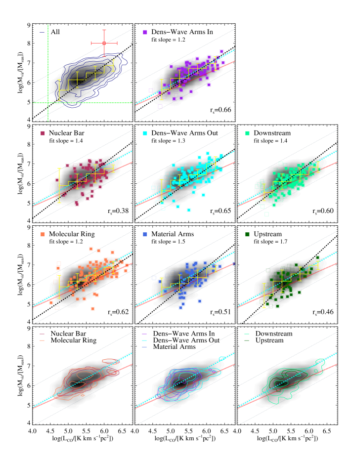
Figure 9: Virial mass-luminosity relation (second Larson’s law) for GMCs in M51 for the various environments. Every column refers to a different region (from left to right: spiral arm, inter-arm and central region). Data points corresponding to clouds with $S/N>6.5$ are highlighted with filled symbols. The shaded area shows the density distribution of the full catalog. Red dotted lines indicate the Galactic fit ($M_{vir}$(M${}_{\odot})=39L_{CO}^{0.81}$(K km s^-1 pc²), S87), cyan dashed lines the extragalactic fit ($M_{vir}$(M${}_{\odot})=7.6L_{CO}^{1.00}$(K km s^-1 pc²), B08) and black dotted lines the fits for the different environments. The slopes of our fits are indicated in the figure panels. Dashed grey lines indicate different $X_{CO}$ values, from bottom to top $X_{CO}=$ $4\times 10^{19}$, $4\times 10^{20}$, and $4\times 10^{21}$ cm^-2 K^-1 km^-1 s. Spearman’s correlation rank is indicated in the bottom right of each panel. The histogram in yellow illustrates the median and the MAD of log($M_{vir}/$[M_⊙]) in bins of 0.5 dex for log($L_{CO}/$[K km s^-1 pc^-2])$\in(4.5-6.5)$. The bottom row shows a contour representation of the GMCs with $S/N>6.5$ within the various environments. In the top left panel the contours show the distribution of the full sample of “high reliable clouds” (with $S/N>6.5$). Green lines indicate resolution limit: $2.7\times 10^{4}$ K km s^-1 pc^-2 for CO luminosity and $9.3\times 10^{4}$ $M_{\odot}$ for the virial mass. The average error bars are reported in red in the top right corner of the top right panel.

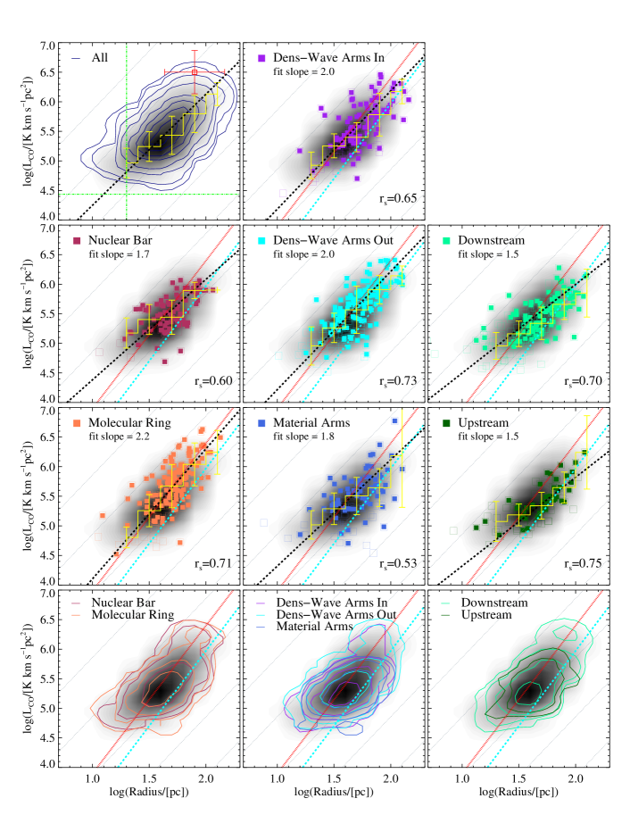
Figure 11: Luminosity-size relation (third Larson’s law) for GMCs in the various M51 environments. Every column refers to a different region (from left to right: spiral arm, inter-arm and central region). Data points corresponding to clouds with $S/N>6.5$ are highlighted with filled symbols. The shaded area shows the density distribution of the full catalog. Red dotted lines indicate the Galactic fit ($L_{CO}$(K km s^-1 pc²)=$25R^{5}$(pc), S87), cyan dashed lines the extragalactic fit ($L_{CO}$(K km s^-1 pc²)=$7.8R^{2.54}$(pc), B08) and black dotted lines the fits for the different environments, which slopes are directly indicated in the figure panels. Dashed grey lines indicate different H₂ surface density values, from bottom to top $\Sigma_{H_{2}}=$ 1, 10, 100, 10³, and 10⁴ M_⊙ pc^-2. At the bottom of the panels the Spearman’s correlation rank is indicated. The histogram in yellow illustrates the median and the MAD of log($L_{CO}/$[K km s^-1 pc²]) in bins of 0.2 dex for log(R/[pc])$\in(1.2-2.0)$. The bottom row shows a contour representation of the various environments. In the top left panel the contours show the distribution of the full sample of reliable clouds (with $S/N>6.5$). Green horizontal and vertical lines indicate the nominal sensitivity and resolution limits: $2.7\times 10^{4}$ K km s^-1 pc^-2 for CO luminosity and 20 pc for the radius, respectively. The average error bars are reported in red in the top right corner of the top right panel.

To estimate the degree of correlation between GMC properties we calculate the Spearman’s rank correlation coefficient (Spearman C 1904). This coefficient, $r_{s}$, assesses how well the relationship between two variables can be described by a monotonic function. If there are no repeated data values, +1 indicates a perfect monotonically increasing function. We consider the properties to be strongly correlated if $r_{s}\geq 0.8$, and moderately correlated if $0.5<r_{s}<0.8$. For the scaling relations shown in Fig. 9 and Fig. 11, the corresponding $r_{s}$ values are indicated in the bottom corner of each panel.

To fit any correlations that we detect, we use the IDL implementation distributed by Erik Rosolowsky of the “BCES” (bivariate, correlated errors with intrinsic scatter) method described by Akritas & Bershady 1996. The BCES bisector estimator takes into account the uncertainty associated with each cloud property measurement. In our estimate for the best-fitting relation, we use only the “highly reliable sample” of clouds of the catalog, i.e. GMCs with $S/N>6.5$ (see Section 4), and we assume that the measurement uncertainties are uncorrelated.

6.1 First Larson’s law: size-velocity dispersion relation

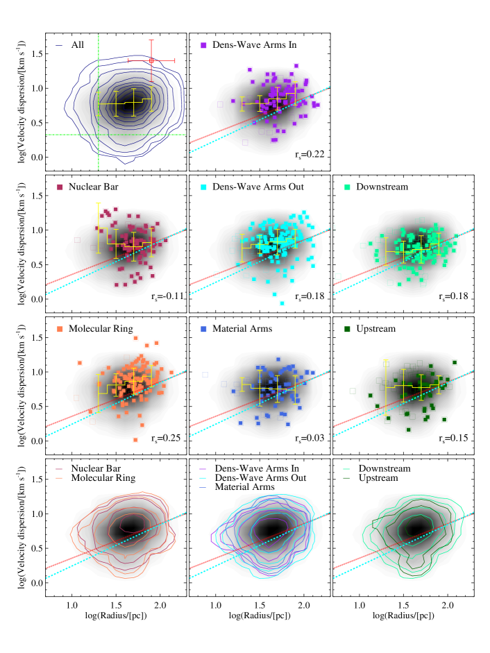
Figure 8: Size-velocity dispersion relation (first Larson’s law) for GMCs in M51 within the various environments. Every column refers to a different region (from left to right: spiral arm, inter-arm and central region). Data points corresponding to clouds with $S/N>6.5$ are highlighted with filled symbols. The shaded area shows the density distribution of the full catalog. Red dotted lines indicate the Galactic fit ($\sigma_{v}(km/s)=0.72R(pc)^{0.5}$, S87) and cyan dashed lines the extragalactic fit ($\sigma_{v}(km/s)=0.44R(pc)^{0.6}$, B08). In the bottom right corner of each panel the Spearman’s correlation rank is given. The histogram in yellow illustrates the median and the MAD of log($\sigma_{v}$/[km/s]) in bins of 0.2 dex for log(R/[pc])$\in(1.0-2.0)$. Then bottom row shows a contour representation of all GMCs with $S/N>6.5$ within the various environments. In the top left panel the contours show the distribution of the full sample of “highly reliable clouds” (with $S/N>6.5$). Green horizontal and vertical lines indicate the nominal resolution limit: 20 pc (CLEAN beam radius) and 2.12 km/s (channel velocity dispersion). The average error bars are reported in red in the top right corner of the top right panel.

The relationship between the size and velocity dispersion of GMCs in the PAWS catalog is shown in Fig. 8. For all environments, there is a high degree of scatter and the $r_{s}$ values indicate that the size and linewidth of the M51 GMCs are, at best, weakly correlated. If we restrict our comparison to GMCs with high signal-to-noise ($S/N>6.5$), then a linear trend between $R$ and $\sigma_{v}$ becomes apparent for some environments, although the correlation is still very weak ($r_{s}\leq 0.25$). In the bottom row of Fig. 8, we use contours to indicate the region of the size-velocity dispersion space occupied by GMCs in different M51 environments. Compared to spiral arm environments, the inter-arm region lacks clouds with high $\sigma_{v}$, while GMCs in the central region seem shifted slightly towards higher values of $R$ and $\sigma_{v}$. It is worth to note also that the majority of the data points lies above the Galactic (S87) and extragalactic (B08) fits, in particular in the case of the center and spiral arm samples. This shows that GMCs in M51 have a higher velocity dispersion compared with similar size clouds in the Milky Way or Local Group galaxies.

6.2 Second Larson’s law: virial mass-luminosity relation

In Fig. 9, we plot the virial mass of the M51 GMCs as a function of their CO luminosity. We note that both virial mass and CO luminosity depend on a combination of $R$ and $\sigma_{v}$, i.e. $M_{vir}\propto\sigma_{v}^{2}R$ and $L_{CO}\propto\langle T\rangle R^{2}\sigma_{v}$, so a significant degree of correlation between these quantities is expected. Fig. 9 shows that GMCs in M51 are scattered around the extragalactic relation obtained by B08 ($M_{vir}$(M_⊙)=$7.6L_{CO}^{1.00}$(K km s^-1 pc²)), although the peak-to-peak variations in $M_{vir}/L_{CO}$ span up to $\sim 2$ orders of magnitude. The best-fitting mass-luminosity relations that we obtain for the different M51 GMC populations are steeper than the B08 relation by $\sim 0.2$ to 0.5 dex. We note that the slope of the mass-luminosity relation varies with environment, increasing from $\sim 1.3$ in the spiral arm and central regions to $\sim 1.5$ in the inter-arm region. This increment is likely driven by differences in luminosity and velocity dispersion observed within the environments. Nevertheless, the clouds appear roughly distributed around a $X_{CO}=4\times 10^{20}$ cm^-2 (K km s^-1)^-1, consistent with the average value that has been observed for other nearby galaxies (e.g. Blitz et al. 2007, B08).

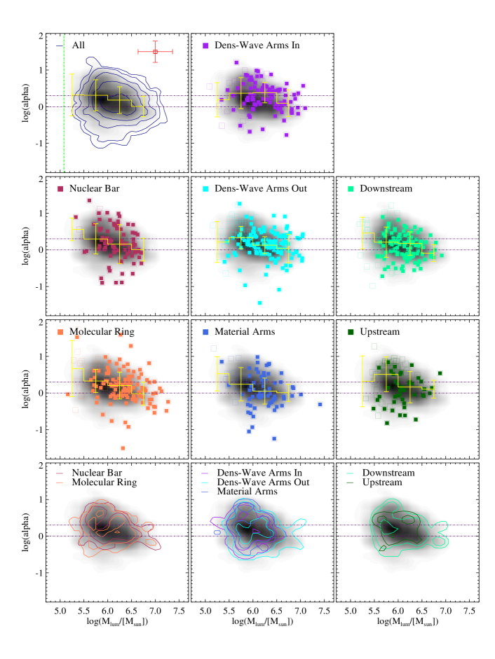
Figure 10: Mass-virial parameter relation for GMCs in the various M51 environments. Every column refers to a different region (from left to right: spiral arm, inter-arm and central region). Data points corresponding to clouds with $S/N>6.5$ are highlighted with filled symbols. The shaded area shows the density distribution of the full catalog. The histogram in yellow illustrates the median and the MAD of log($\alpha$) in bins of 0.5 dex for log($M_{lum}$/[M${}_{\odot}]\in(5.0-7.0)$. The bottom row shows a contour representation of the GMCs with $S/N>6.5$ within the various environments. In the top left panel the contours show the distribution of the full sample of “highly reliable clouds” (with $S/N>6.5$). Purple horizontal dashed lines indicate the limit between self-gravitating and pressure confined clouds ($\alpha=1$) and unbound clouds ($\alpha=2$). Green line indicates our nominal sensitivity limit: $2.7\times 10^{4}$ K km s^-1 pc^-2 for CO luminosity. The average error bars are reported in red in the top right corner.

The analysis of the distribution of the virial parameter of Section 5.3.2 has shown that clouds in M51 are in general self-gravitating. Here we check if $\alpha$ is correlated with the cloud mass. In Fig. 10, we plot $\alpha$ as a function of $M_{lum}$ finding that although GMCs with $\alpha>2$ are present across our entire observed mass range, the average value of $\alpha$ tends to decrease for high mass clouds. This plot should be interpreted with care, since the axes are correlated ($M_{lum}$ appears in the denominator of the virial parameter definition). Nevertheless, since there are low- to intermediate-mass clouds with high signal-to-noise and large virial parameters ($\alpha>2$), Fig. 10 suggests that overall the high mass clouds in M51 tend to be more strongly bound than low mass clouds.

6.3 Third Larson’s law: Luminosity-size relation

Fig. 11 shows that the size and CO luminosity of M51 GMCs are strongly correlated, with $0.5<r_{s}<0.8$. This is not surprising since $L_{CO}\propto\langle T\rangle R^{2}\sigma_{v}$. The bottom row of Fig. 11 shows that the relationship between $R$ and $L_{CO}$ is steeper in the central and spiral arm regions than in the inter-arm region. This is confirmed by the results of a linear regression fit: the slope of the best-fitting power law flattens from 2.4 for GMCs in the molecular ring, to $\sim 2$ for clouds in the density wave spiral arms, to $<1.5$ for the inter-arm environments. The origin of such effect is likely to be the different CO emission properties within the different M51 environments (such as the geometry, CO filling factor and/or density distribution, see also Hughes et al. 2013b) but further investigation into its physical significance is required. Nevertheless, the change in slope of the fit appears to be real, given the fact that all environments span a similar range of GMC radii but contain clouds with very different luminosity. Assuming a uniform $X_{CO}$ factor throughout the PAWS field, the linear regression illustrates why the median H₂ mass surface density varies with environment: large GMCs located in molecular ring and density-wave spiral arms contain more high brightness CO emission than clouds of an equivalent size in the inter-arm region.

6.4 CPROPS bias corrections and scaling relations

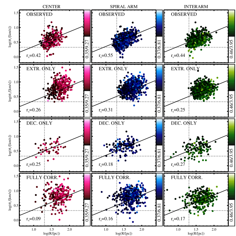
Figure 12: Comparison of the Larson’s laws for observed (top row), extrapolated only (second row), deconvolved only (third row) and fully corrected (extrapolated and deconvolved, bottom row) properties of the full GMC catalog. The three columns present the central (left), arm (middle) and inter-arm (right) GMC populations. Spearman’s rank correlation coefficients ($r_{s}$) of the full catalog are indicated at the bottom left of each panel. Straight dotted lines indicate resolution limits: 2.12 km s^-1 channel “velocity dispersion” and 20 pc beam “radius”. The full black line represents the Galactic fit by S87.

Although Larson’s Laws have regularly been used as yardstick for comparing GMC populations, a number of previous studies have demonstrated that the method used to identify clouds and measure their properties has a large impact on the appearance of the Larson-type scaling relations (e.g. Wong et al., 2011). In Section 5.4, we argued that the CPROPS bias corrections are important for recovering a reliable estimate for the properties of GMCs within the PAWS field. In Fig. 12, we plot the size-linewidth relation for the PAWS clouds in the three main environments, using measurements with and without the resolution and sensitivity corrections applied. It is clear that the uncorrected properties (top row) exhibit the most robust correlations. Taken individually, the corrections for sensitivity (i.e. extrapolation, second row) and resolution (i.e. deconvolution, third row) appear to introduce a comparable level of scatter into the size-linewidth relation, decreasing the Spearman rank correlation coefficient by a factor of $\sim 2$ with respect to the relation exhibited by the uncorrected properties. It is important to recall, however, that the observed objects are not uniformly defined across the PAWS field: the CO brightness at the cloud boundary tends to be higher for objects in the spiral arm region ($\langle T_{edge}\rangle\in[0.4,6.8]$ K, middle column) than for the inter-arm ($\langle T_{edge}\rangle\in[0.5,4.0]$ K, right column). The top row of Fig. 12 shows that these differences in the definition of the cloud lead to some segregation of the data points within the size-linewidth plot, i.e. objects with low brightness boundaries (darker points) tend to have larger linewidths relative to their size than objects with boundaries at a higher brightness threshold (lighter points). In summary, our analysis re-inforces conclusions from previous observational studies that the methods used to identify GMCs and measure their properties exerts a significant influence over the existence and slope of a size-linewidth relation, and that decomposition methods that use a fixed brightness threshold to define cloud boundaries seem to yield stronger size-linewidth relations. This should be kept in mind by studies that collate literature values to, e.g., compare the physical properties of extragalactic GMC populations, or validate physical models for the origin of the first Larson Law.

7 GMC Mass spectra

7.1 Construction and general properties

The GMC luminosity distribution depicts how the CO flux is organized into clouds of different luminosity within a galaxy (e.g. Rosolowsky 2005). In this section, we frame our discussion in terms of the GMC mass spectrum, which equivalently describes how molecular gas is organized into cloud structures of different mass, assuming that CO emission is a reliable tracer of H₂. We convert the CO luminosity to H₂ mass assuming a constant Galactic conversion factor $X_{CO}=2\times 10^{20}$ cm^-2 (K km s^-1)^-1, and including the mass contribution of helium, thus $M_{lum}=4.4L_{CO}$ (eq. 7).

The GMC mass spectrum is usually expressed in differential form and modeled as a power law:

$$f(M)=\frac{dN}{dM}\propto M^{\gamma}$$ (14)

The integral of this expression yields the cumulative mass distribution, i.e. the number of clouds $N$ with masses $M$ greater than a reference mass $M_{0}$ as a function of that reference mass:

$$N(M^{\prime}>M)=\left[\left(\frac{M}{M_{0}}\right)^{\gamma+1}\right].$$ (15)

The index $\gamma$ describes how the mass is distributed: for values $\gamma>-2$, the gas is preferentially contained in massive structures, while for values $\gamma<-2$, small clouds dominate the molecular mass budget.

Several studies have reported that the mass spectrum steepens at high cloud masses (e.g. Fukui et al. 2001, Rosolowsky 2007, Gratier et al. 2012). In this case, it can be useful to model the mass spectra using a truncated power-law (Williams & McKee 1997):

$$N(M^{\prime}>M)=N_{0}\left[\left(\frac{M}{M_{0}}\right)^{\gamma+1}-1\right],$$ (16)

where $M_{0}$ is the maximum mass in the distribution and $N_{0}$ is the number of clouds more massive than $2^{1/(\gamma+1)}M_{0}$, the mass where the distribution deviates from a simple power-law (i.e. the truncation mass).

Fig. 13 shows the cumulative $M_{lum}$ distributions for GMCs in different M51 environments. The equivalent values of CO luminosity are indicated on the top x-axis. In the left panel, the distributions are normalized by the projected area (in kpc²) of the different environments (listed in Table 2, and indicated in the top-right corner of the panels in Fig. 14). Using this normalization, the vertical offsets between the different mass distributions reflect true variations in the number surface density of GMCs: as noted in Section 5.2, the number density of GMCs is higher in the center than the spiral arms, and higher in the spiral arms than the inter-arm region. The right panel of Fig. 13 shows the same GMC mass distributions, this time normalized by the total number of GMCs in each environment to facilitate a comparison of the distribution shapes.

$\begin{array}[]{cc}\includegraphics[width=173.44534pt]{f13.eps}&\includegraphics[width=173.44534pt]{f14.eps}\\ \end{array}$

Figure 13: Cumulative mass spectra for GMCs in the different environments of M51 normalized by the area covered by the environments in kpc² (left; see Fig. 14 for exact area) and to the total number of clouds for each environment (right). The distributions clearly exhibit both a vertical offset in the left panel (i.e. a different number density of GMCs) and a horizontal offset (i.e. a different maximum cloud mass), as well as the different distribution shapes. The equivalent CO luminosity is indicated on the top axis.

The top-left panel of Fig. 14 shows that the overall mass distribution of GMCs within the PAWS field steepens continuously with increasing mass. Comparing this global distribution with those in the other panels of Fig. 14 suggests that the non-power-law shape of the overall distribution is due to combining the intrinsically diverse GMCs mass distributions that characterize different galactic environments. The GMC mass distribution in the inter-arm and material arm environments, for example, can be adequately represented by simple or truncated power-laws across the range of cloud masses probed by PAWS, and are hence more similar to the GMC mass distributions that have been previously observed for M33 and the LMC (Wong et al. 2011, Gratier et al. 2012). Across most of the observed mass range, the slope of the mass distribution is shallower in the molecular ring and the density-wave spiral arms than in the inter-arm, while the mass distribution in the material arms has a slope that is intermediate between these extremes. Extremely high mass objects ($M_{lum}>10^{7}$ $M_{\odot}$) are only observed in the molecular ring and spiral arms. The inter-arm region contains very few clouds with masses greater than $10^{6.5}$ $M_{\odot}$, although the mass distribution of downstream GMCs reaches slightly higher cloud masses than the upstream cloud distribution. The nuclear bar has a high number density of clouds, and shows evidence for a very strong truncation at $10^{6.5}$ $M_{\odot}$.

7.2 Variation in the GMC Mass Distribution with Environment

In the Milky Way and other Local Group galaxies, GMC mass distributions tend to be adequately represented by simple power-laws (e.g. Rosolowsky 2005 and references therein), although previous studies have noted that the cloud mass distribution steepens at high masses in the LMC (Fukui et al. 2008, Fukui & Kawamura 2010) and in M33 (Gratier et al. 2012). In M51, we find that the overall mass distribution steepens continuously with increasing cloud mass above our adopted sensitivity limit $3.6\times 10^{5}$ M_⊙. This is also evident for the GMC mass distributions in the molecular ring and density wave spiral arm environments, while the nuclear bar mass distribution exhibits a strong truncation around $5\times 10^{6}$ M_⊙. To characterize the diverse shapes of the GMC mass distributions and facilitate the comparison between M51 and results from other galaxies, we therefore fit the distributions with Eq. 16 above a relatively high fiducial mass of $10^{6}$ M_⊙, where the mass distributions show more resemblance to a truncated power-law. This limit is significantly higher than our adopted catalog completeness limit and roughly corresponds to the lower mass limit of the highly reliable sample of clouds. We discuss the reasons for only fitting the mass distributions above this relatively high mass, and the possible effects of incompleteness on the mass distributions in Section 7.3. The fit is performed using Erik Rosolowsky’s IDL procedure MSPECFIT, which implements the maximum likelihood method described in Rosolowsky 2007. As a goodness-of-fit test we use the KS test. The parameters of the fits to the mass distributions are summarized in Table 5. The fits are overplotted on the mass distributions in Fig. 14.

The GMC mass spectra belonging to the different environments of M51 show different features. The molecular ring and density-wave spiral arm cloud distributions show similar slopes ($\gamma\approx-1.8$ to $-1.6$) and fitted maximum masses M${}_{0}>$10⁷ M_⊙. The mass distributions from the inter-arm and material arm regions, by contrast, have $\gamma\approx-2.5$. These results indicate that the molecular gas in the molecular ring and density-wave spiral arms is preferentially distributed in high mass GMCs, whereas smaller clouds are the preferred unit of molecular structure in the inter-arm and material arm environments. The case of the nuclear bar spectrum is peculiar, since it presents the shallowest slope ($\gamma\approx-1.3$), but also reveals a sharp truncation for cloud masses above M${}_{0}\approx 5.5\times 10^{6}$ M_⊙.

The inter-arm and material arm spectra have N₀ close to the unity, suggesting that a simple power-law is sufficient to describe the mass distributions. We test this possibility finding that upstream and material arm distributions can be well represented by simple power-laws, as shown by the p-values of the corresponding KS tests, which are close to 1. Even a truncated power-law, however, does not provide a good fit for overall M51 distribution. This is not surprising since the distribution for GMCs within the whole PAWS field is composed of the superposition of the mass distributions from the different M51 environments, which have different slopes and different truncation masses.

The mass- and environment-dependent variations in the M51 GMC mass distributions suggest that different mechanisms regulate the formation and destruction of GMCs in different regions of M51’s inner disk. The non-power-law shape of the mass distributions, which is most pronounced in the central and density-wave spiral arm environments, is suggestive of processes that promote the formation (and survival) of intermediate and high mass clouds. The mass distributions in the inter-arm region (especially upstream) are closer to pure power-laws, suggesting that the mechanism(s) responsible for the curvature in the mass distributions is not as effective in the inter-arm. The influence of spiral structure on a GMC ensemble may therefore provide another possible explanation for why the generic shape of the GMC mass distribution in M51 is distinct from the simple power-law observed for other extragalactic GMC populations, which tend to be from low-mass dwarf galaxies (e.g. the LMC and M33, Wong et al. 2011, Gratier et al. 2012) or regions of galactic disks without strong spiral structure (e.g. the outer Milky Way and an outer arm of M31, Rosolowsky 2005). We discuss a possible origin for the environment-dependent changes in the shape of the mass distribution in Section 8.

Table 5: Truncated power-law fits to the GMC mass spectra in different M51 environments

Envir.	$\gamma$	M0	N0	p-value
		$10^{6}$ M⊙
All	$-2.29\pm 0.09$	$18.5\pm 3.4$	$17\pm 7$	$10^{-4}$
NB	$-1.33\pm 0.21$	$5.2\pm 0.3$	$90\pm 21$	1.00
MR	$-1.63\pm 0.17$	$15.0\pm 3.2$	$26\pm 20$	0.72
DWI	$-1.75\pm 0.20$	$12.2\pm 1.8$	$15\pm 12$	1.00
DWO	$-1.79\pm 0.09$	$11.8\pm 0.9$	$24\pm 9$	0.30
MAT	$-2.52\pm 0.20$	$158.6\pm 7.4$	$0\pm 2$	0.92
UPS	$-2.44\pm 0.40$	$9.3\pm 4.0$	$2\pm 3$	1.00
DNS	$-2.55\pm 0.23$	$8.3\pm 1.9$	$5\pm 4$	0.36

Slopes $\gamma$, maximum mass $M_{0}$ and number of GMCs at the maximum mass $N_{0}$ of the truncated power-law fits to the GMC mass spectra of the different environments in M51. The error are obtained through 50 bootstraps interaction. In the last column, we list the p-values of the KS tests as an indication of the goodness-of-fit.

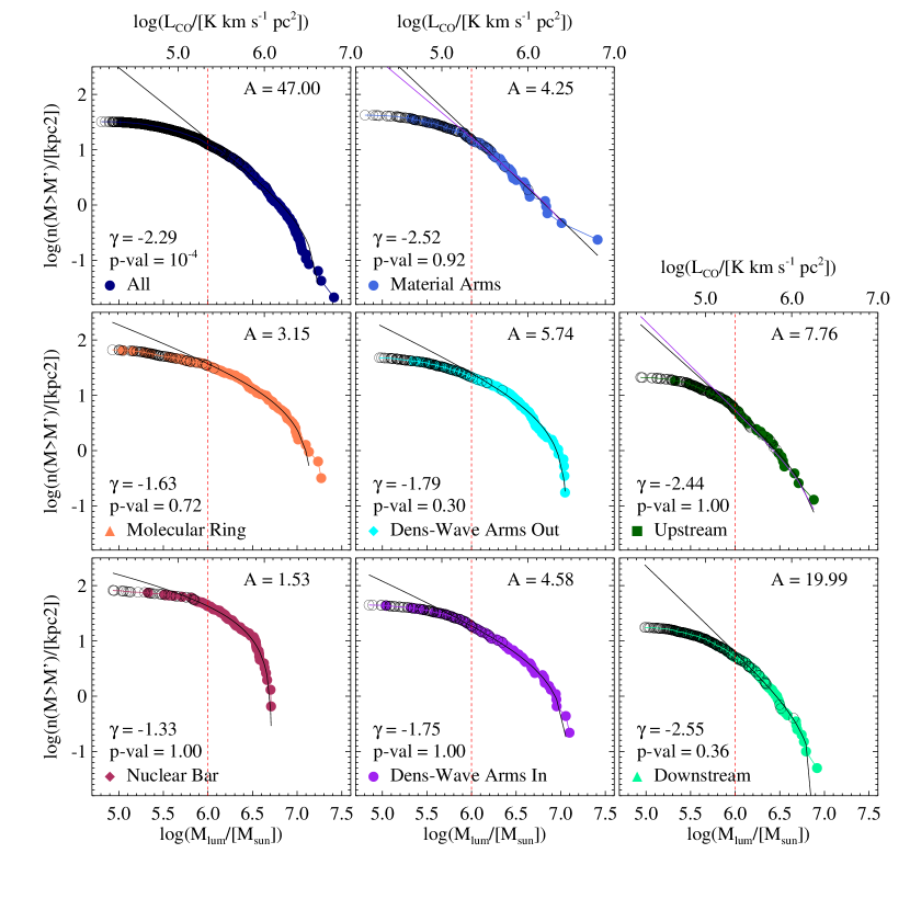
Figure 14: Cumulative mass spectra for GMCs in the different environments (from left to right: central, spiral arm, inter-arm regions with the full catalog shown in the top left panel). Colored full circles indicates clouds within the “highly reliable sample”, while empty black circles clouds with $S/N<6.5$. Solid black lines represent the truncated power-law fits while the purple line indicates the power-law fits for distributions that show resemblance with simple power-law. The red vertical dashed line indicates the lower mass limit of the fit ($10^{6}$ M$\odot$). In the top-right corner of each panel the normalization area “A” ( in kpc²) is given, while on the lower-left corner the value of the slope ($\gamma$) and of the KS test p-value (p-val) are indicated. For reference, the top axis provides the equivalent CO luminosity.

7.3 Testing the Shape of the GMC Mass Distributions for Incompleteness Effects

As we noted in Section 7, most extragalactic GMC mass distributions that have been observed to date are adequately represented by a simple or truncated power-law. Since we argue that the shape of the mass spectrum yields important clues regarding the physical mechanisms of cloud formation and destruction, it is important to assess whether the mass distributions that we obtain are reliable. In particular, although the mass corresponding to the sensitivity limit of our observations ($\sim 10^{5}$ M_⊙) suggests that our GMC catalog should be reasonably complete above $3.6\times 10^{5}$ M_⊙, CPROPS might still be unable to distinguish clouds above this mass if they are located in a crowded region like the spiral arms, effectively raising the completeness limit.

To test whether the observed GMC mass distributions in M51 could be significantly affected by incompleteness, we estimated the total number of GMCs with masses $M>10^{5.5}$ M_⊙ and their combined CO luminosity that would be expected in each M51 environment if: (i) the true mass distribution followed a simple power-law with the same exponent as in the intermediate mass bin down to $M=10^{5.5}$ M_⊙ (case A); and (ii) the true mass distribution across the mass range followed a simple power-law with the same exponent as in the upper mass bin down to $M=10^{5.5}$ M_⊙ (case B). A schematic explaining the two cases is shown in Figure 15, and the results for each M51 environment are presented in Table 6.

$\begin{array}[]{cc}\includegraphics[width=199.16928pt]{f16.eps}&\includegraphics[width=199.16928pt]{f17.eps}\\ \end{array}$

Figure 15: Schematic diagram illustrating our test for whether there is a genuine steepening of the GMC mass distributions in M51. We calculate the total number of GMCs under the assumption that the power-law mass distribution observed [a] across the mass range $\log(M)\in[6.0,6.5]$ (case A) or [b] across the mass range $\log(M)\in[6.5,7.0]$ continues down to $M=10^{5.5}$ M_⊙. The shape of the distribution at higher GMC masses is assumed to follow the observed distribution. The grey shaded wedge in each panel indicates the difference between the power-law distribution (red dashed line) and observed mass distribution (black solid line) in each case. To test whether the true GMC mass distribution could be consistent with the power-law mass distribution, we examine whether the total CO luminosity corresponding to the power-law mass distribution exceeds the integrated CO flux and working area flux within each M51 environment.

On one hand, it is clear that there must be a genuine steepening of the GMC mass distribution in all M51 environments. If the mass distributions in the inner spiral arms and molecular ring were simple power-laws with the same exponents that we observe across the mass range $10^{6.5}$ to $10^{7}$ M_⊙(i.e. case B), then the total number of GMCs with $M>10^{5.5}$ M_⊙ in each environment would exceed several thousand, and the CO luminosity associated with this mass distribution would be greater than each region’s total CO flux (measured via direct integration of the PAWS data cube) by factors between five and ten. A similar – though not identical – situation applies in the material arm and inter-arm regions. The CO luminosity corresponding to a power-law mass distribution for GMCs with $M>10^{5.5}$ M_⊙ with the same exponent as that in the intermediate mass bin would not exceed (or, in the case of the material arm, would not greatly exceed) the total CO flux of these regions, but it would require that roughly half of the undetected GMCs fall outside the CPROPS ‘working area’, i.e. the initial mask identifying regions of significant emission. As such, these undetected GMCs would need to be spatially extended, low CO surface brightness structures containing $10^{5.5}$ to $10^{6}$ M_⊙ of CO-emitting molecular gas without an emission peak brighter than $4\sigma_{RMS}=1.2$ K. Since the total CO luminosity associated with this mass distribution is comparable to the total flux of these regions, moreover, it would also entail a strong flattening of the GMC mass distribution for $M<10^{5.5}$ M_⊙. A more gradual flattening of the GMC mass distribution between $10^{5.0}$ and $10^{6}$ M_⊙ would seem at least as plausible as the possibility that high-mass, low-surface brightness structures are ubiquitous throughout M51’s inter-arm and material arm while clouds with $M<10^{5.5}$ M_⊙ are intrinsically rare.

On the other hand, we cannot use similar arguments to rule out that the slope of the GMC mass distributions between $10^{5.5}$ to $10^{6}$ M_⊙ in the spiral arm and central regions could be due to an algorithmic effect. If the mass distribution in these regions continued with the same exponent that we observe for the intermediate mass bin down to $10^{5.5}$ M_⊙ (or even $10^{5.0}$ M_⊙), then the constraint that the combined CO luminosity should not exceed the observed CO flux is not violated. Indeed, the combined CO luminosity that would be associated with GMCs with $M>10^{5.0}$ M_⊙ assuming a simple power-law across $10^{5.0}$ to $10^{6.5}$ M_⊙ is less than or comparable to the flux in the working area (i.e. not only the total flux) for these environments.

Nevertheless, moving the completeness limit up to $10^{6}$ M_⊙ does not change our main conclusions about the different physical mechanisms that regulate the formation/disruption of GMCs, which we infer mainly from the intermediate and upper mass bins of the mass spectra. We further note that considering only clouds with $M_{lum}>10^{6}$ M_⊙  makes the differences in the cloud properties described in Sections 5.3.1-5.3.2 even more pronounced.

Table 6: Results of GMC Mass Distribution Tests

Region	$L_{CO}$ in Environment		Observed Distribution		Case A		Case B(a)
	Total	Working Area	$N_{GMCs}^{(b)}$	$L_{CO}^{(c)}$	$N_{GMCs}^{(b)}$	$L_{CO}^{(c)}$	$N_{GMCs}^{(b)}$	$L_{CO}^{(c)}$
	$[10^{7}\,{{\rm\thinspace K\thinspace km\thinspace s}^{-1}\thinspace{\rm pc}^{2}}]$	$[10^{7}\,{{\rm\thinspace K\thinspace km\thinspace s}^{-1}\thinspace{\rm pc}^{2}}]$		$[10^{7}\,{{\rm\thinspace K\thinspace km\thinspace s}^{-1}\thinspace{\rm pc}^{2}}]$		$[10^{7}\,{{\rm\thinspace K\thinspace km\thinspace s}^{-1}\thinspace{\rm pc}^{2}}]$		$[10^{7}\,{{\rm\thinspace K\thinspace km\thinspace s}^{-1}\thinspace{\rm pc}^{2}}]$
Cube	90.83	67.08	1160	47.05	2207	59.25	27739	407.9
NB	7.48	6.49	116	5.07	270	6.96
MR	17.99	16.35	160	9.60	315	11.44	5082	79.34
DWI	13.13	11.23	180	7.58	280	8.75	9057	126.39
DWO	18.38	15.73	260	11.73	371	12.76	8290	122.21
MAT	8.06	5.44	148	5.64	537	10.36	825	14.19
DNS	17.96	8.54	156	4.40	566	9.34
UPS	7.79	3.28	140	3.03	478	7.03

Note. — (a) Only for environments with a maximum GMC mass greater than $10^{7}$ M_⊙; (b) number of GMCs with $M>10^{5.5}$ M_⊙ in the distribution; (c) combined CO luminosity of GMCs with $M>10^{5.5}$ M_⊙(see text for details).

8 Discussion

8.1 An Evolutionary Scenario for the Environmental Variation of the GMC Mass Distributions in M51

Recent studies of GMCs and their associations, i.e GMAs, in nearby disk galaxies have provided evidence that cloud properties are not uniform across the disk and that galactic environment (such as bulge, disk, nuclear bars, star-forming rings, spiral arms and inter-arm regions) might be responsible for the observed differences. Koda et al. (2009), for example, find that GMAs with masses above $\rm 10^{7}\,M_{\sun}$ are exclusively located along the spiral arms of M51. They attribute this observed spatial distribution to large-scale dynamical processes induced by the spiral potential. In a recent sample of five nearby galaxies from the CANON survey, a similar trend for massive GMCs to be associated with strong spiral arms is observed (e.g. Fig. 6 of Donovan Meyer et al. 2013). The differences in M51’s GMC properties with galactic environment that we describe in this paper are therefore not entirely unexpected. However, our study provides the first quantitative measure of the differences in the cloud properties and also reveals a strong variation in the GMC mass spectra (i.e. slope, normalization and maximum mass; Section 7.2) with galactic environment. The variations in the mass spectrum are observational signatures of the mechanisms of cloud formation and evolution, providing evidence for processes that not only change the physical properties of individual clouds, but also influence the ensemble properties of the cloud population.

The mass spectra of clouds in the inter-arm and density-wave spiral arm are different. The variation in the slope $\gamma$ between the density-wave spiral arm and upstream mass spectra (Section 7.2) implies that spiral arms do not simply gather GMCs from the upstream inter-arm environment (in this case the slope of the mass distributions would be identical, even though the overall normalization could change), but also modify the nature of the constituent clouds. More precisely, the inter-arm distributions are steep (spectral index $\gamma<-2$) and all clouds have masses lower than 10⁷ M_⊙, characteristic of a population of clouds that is dominated by low-mass objects. The spiral density wave mass spectra, by contrast, are shallower ($\gamma>-2$) and have a much higher maximum cloud mass, consistent with a cloud population mainly constituted by high mass objects. Spiral arms, therefore, must host processes that promote the growth of massive clouds, without providing an effective mechanism for their destruction.

Within a spiral potential, Jeans instabilities are thought to be the dominant mechanism of cloud formation (e.g. McKee & Ostriker 2007). Numerical studies of gas in spiral potentials have observed that GMCs also increase their mass through coagulation processes (cloud collisions, accretion of small clouds, mutual coalesence) that are aided by the converging streamlines of the gas flow within the arms (Casoli & Combes 1981, Kwan & Valdes 1983, Tomisaka 1986, Dobbs 2008, Tasker & Tan 2009). Together with those phenomena, Meidt et al. (2013) proposed that streaming motions associated with the spiral potential decrease the external gas pressure leading to increased stable masses (see also Jog 2013). Therefore, GMCs in regions of the spiral arm with strong streaming motions can become very massive without undergoing significant collapse. A recent numerical simulation by Dobbs & Pringle (2013) of a two armed spiral galaxy that includes a spiral potential, self-gravity, heating and cooling of the ISM and stellar feedback (see Fig. 16) yields mass spectra that are similar to those observed for the spiral arm and inter-arm region of M51. In this simulation, cloud formation is a complex process that involves gravitational instabilities, assembly of smaller clouds and accretion of local interstellar gas onto the cloud. However, we note that the number density of clouds across the entire observed mass range increases within the spiral arm environments, i.e. low mass clouds are also created in the arms and not just subsumed into larger structures. This suggests that gravitational instabilities remain the primary mechanism for GMC formation in M51’s spiral arms, although dynamical effects almost certainly play an important role in bringing a large quantity of molecular gas to a single location, where it subsequently fragments due to gravitational instabilities.

Koda et al. (2009) have argued that GMCs in the inter-arm regions of M51 cannot have formed locally on an inter-arm crossing time-scale, but are rather remnants of GMCs that were previously in the spiral arms. The change in the GMC mass distribution between the arm and inter-arm region suggests that GMCs undergo a disruptive process (or processes) that preferentially affects the most massive objects when they leave the arms. Numerical simulations of the ISM in spiral galaxies (Dobbs et al. 2006, Dobbs & Pringle 2013) suggest that the prominent “spurs” that emanate downstream from the spiral arms (see La Vigne et al. 2006, Schinnerer et al. 2013) can be interpreted as sheared GMCs or their associations due to large-scale dynamical motions. Another possible cause of cloud destruction is feedback from star formation. In M51, young stellar clusters and enhanced atomic gas (HI, CII) emission (Schinnerer et al. 2013) suggest that star formation is enhanced downstream of the outer density-wave spiral arms. Furthermore, there is an extended, dynamically hot component of the molecular gas in M51 (described by Pety et al. 2013) that spatially correlates with locations of star formation, and could be the result of galactic fountains or chimneys that have transported some of the molecular gas away from the disk (e.g. Putman et al. 2012). Yet star formation feedback cannot be the primary cause for cloud disruption throughout M51’s spiral arms since the inner spiral arm segments have no evidence for high mass star formation (Schinnerer et al. 2013). The cloud mass distributions in the inner and outer arms are very similar, suggesting either that star formation feedback is not the dominant destruction mechanism in any of the arm environments or that shear and star formation feedback yield a similar mass distribution of cloud fragments upon the disruption of a high mass GMC.

Subtle differences between the upstream and downstream GMC mass distributions (i.e. the higher number density of low-mass upstream clouds with respect to the downstream ones) suggest that the disruptive events continue to act across the entire inter-arm region. If GMCs (not the molecular gas itself) are indeed “short-living” entities ($\sim 30$ Myr, Elmegreen 2000), then they are unable to maintain their identity throughout the whole journey from one arm to the other (e.g. Pringle et al. 2001) causing a transformation of the cloud population to include a higher proportion of low mass objects. Shearing forces are strong throughout the inter-arm region, and therefore likely to play a role in cloud destruction. Star formation, as traced by H$\alpha$ emission, is not entirely absent from the inter-arm region however, suggesting that feedback also contributes to cloud destruction in this region.

The molecular ring is an environment that appears very favorable for cloud formation: the mass distribution in this region is very shallow ($\gamma\approx-1.6$) and extends to cloud masses greater than $10^{7}$ M_⊙. The similarity between the distributions in the molecular ring and the density-wave arm environments would seem to suggest that cloud formation and destruction mechanisms may be present. However, the gas dynamics in the central region are very different from the disk. The molecular ring is coincident with a zero torque environment caused by the overlap of resonances of the inner bar and the spiral density wave, i.e. the combined action of outflow driven by the nuclear bar and inflow by the spiral wave (Meidt et al. 2013). Thus, the molecular ring zone harbors nearly circular orbits with at most low non-circular motions (Colombo et al., submitted) and almost no shear (analogous to the 5 kpc molecular ring in the Milky Way, Dib et al. 2012). Streaming motions in the ring are low, moreover, implying that the stable mass against cloud collapse is determined solely by the gas density. Unlike in the inner spiral arms, high-mass star formation is active throughout the ring and appears coincident with regions of high gas surface density. We propose that due to the opposing action of the bar and spiral arm torques, gas accumulates and stalls in the molecular ring, where it develops high densities. Gravitational instabilities then cause the gas to fragment into clouds. In the absence of shear, star formation feedback should be the dominant mechanism of cloud destruction in this region.

Finally, the formation and destruction of clouds in the nuclear bar environment may also follow a different path than in other parts of the PAWS field. In particular, Figure 13 shows the mass spectrum in the nuclear bar region has a high number density of low and intermediate mass GMCs, but a sharp truncation at around $10^{6.5}$ $M_{\odot}$. This implies that the bar environment either lacks an efficient mechanism to bring small clouds together to form larger structures, or that a very efficient mechanism for the destruction of massive objects is active. The presence of low and intermediate mass GMCs may be a consequence of the abundant molecular gas reservoir collected by the nuclear bar dynamics: gas on the leading sides of a bar loses angular momentum and is driven inwards, as a result of negative gravitational torques (e.g. Schwarz 1984). This motion is also expected to generate intense shear in the gas lanes (e.g Athanassoula 1992, Sheth et al. 2002) that could prevent the formation of massive objects through the inhibition of the density fluctuations that become the seeds of massive GMCs (Hopkins 2012).

Besides the dynamical processes discussed above, other effects, such as variations in the interstellar radiation field (ISRF), the molecular gas fraction and/or the $X_{CO}$ factor, could potentially alter the properties of the M51 GMC populations. In M51, the ISRF is decreasing from the bulge to the disk and, in particular, the intense radiation field of the young massive stars in the star-forming ring and/or the AGN could have a strong impact on cloud disruption and heating of the molecular gas. Beyond the bulge region, however, H-band observations indicate that there is no overall radial trend in the ISRF for the range of galactocentric radii probed by PAWS (Muñoz-Mateos et al. 2011). The molecular gas fraction (defined as $2N_{H_{2}}/(2N_{H_{2}}+N_{HI}$) over the PAWS area is very high ($\sim 0.85$, assuming $X_{CO}=2\times 10^{20}$ cm^-2 (K km s^-1)^-1) and does not significantly vary with radius or azimuth (see e.g. Fig. 2c in Koda et al. 2009). This high molecular fraction is determined mostly by the scarcity of HI emission within the PAWS field; halving the adopted value of $X_{CO}$ only lowers the molecular fraction to $\sim 0.7$. The metallicity and the gas-to-dust ratio within the PAWS FoV also suggest that variations in the $X_{CO}$ factor are unlikely to be the main driver of the differences in the GMC properties and mass spectra that we observe. Bresolin et al. (2004), and Moustakas et al. (2010) both found a metallicity close to solar with only a shallow radial gradient of $\rm-(0.02\pm 0.01)\,dex\,kpc^{-1}$, so we do not expect metallicity-dependent variations in the conversion factor across the PAWS FoV (see e.g. Leroy et al 2011, 2012). A recent analysis of the Herschel FIR continuum (Mentuch Cooper et al. 2012) has likewise shown that the gas-to-dust ratio is roughly constant within the inner 13 kpc of M51, assuming $X_{CO}=2\times 10^{20}$ cm^-2 (K km s^-1)^-1 throughout M51. If there were strong environmental variations in the $X_{CO}$ factor within the PAWS FoV, these would lead to corresponding spatial variations in their derived gas-to-dust ratio map, but such variations are not observed (see Fig 16 in Mentuch Cooper et al. 2012).

In conclusion, the presence of spiral arms has a dramatic effect on the GMC properties observed in the central 9 kpc of M51. Excluding phenomena such as a varying ISRF, molecular gas fraction and $X_{CO}$ factor that are observed to be roughly constant across the disk, we propose that a large amount of gas is accumulated by the spiral arm dynamics, and subsequently fragmented by gravitational instabilities. We further propose that the variations in the shape of the cloud mass spectra can be interpreted as the evolution of clouds traveling from one side of a spiral arm to the other arm. However, further work is required to understand the relative importance of shear and star formation feedback between and within M51’s inner spiral arms, and to characterize the effect of these destruction processes on the shape of the GMC mass distributions. The presence of high mass objects in the circumnuclear ring can be best explained by gas accumulation and strong gravitational instabilities in the absence of strong destructive dynamical effects such as shear. It is likely that shear helps prevent the formation of massive clouds in the nuclear bar region, but the enhanced ISRF in M51’s bulge and the AGN make it difficult to separate their contribution from large-scale dynamical effects in this region.

Figure 16: The cumulative mass distributions for the arm (blue) and inter-arm (green) regions in a simulation of a two armed spiral galaxy. The simulation is described in Section 7 of Dobbs et al. (2012) and is presented in Dobbs & Pringle (2013). The mass per particle was 312.5 M_⊙. Clouds were identified using a clump-finding algorithm that selects contiguous regions with $>25$ M_⊙ pc^-2, an approach that is not dissimilar to CPROPS.

8.2 Larson’s laws in M51

In addition to the differences in the GMC mass spectra with galactic environment, the scaling relations between cloud properties provide further insight into the processes that regulate their physical properties. From our analysis in Section 6, two important features of GMCs in M51 emerge: first, both the size-velocity dispersion and CO luminosity-virial mass relations show a large scatter; and second, the GMC mass surface density varies with environment as seen by the radius-CO luminosity relation. Here, we argue that these results have a common origin, i.e. the different dynamical properties of the environments.

A relation between size and velocity dispersion was identified in the early studies of Milky Way clouds (e.g. Solomon et al. 1979; Larson 1981; Dame et al. 1986). It is often interpreted as evidence for a cloud in virial equilibrium following the work of S87, where the authors measured a square-root dependency between velocity dispersion and radius of Galactic GMCs. But unlike the tight size-velocity dispersion relation discovered by S87, the corresponding relationship in M51 shows a large scatter. If GMCs are not strongly bound, then they become susceptible to modification and/or disruption by events and conditions in the surrounding interstellar medium. For clouds where $\alpha\gg 1$, external sources of confining pressure, such as ram pressure from inflowing material (e.g. Heitsch et al., 2009) or the (static) weight of the surrounding gas (e.g. Heyer et al., 2001) become important for their dynamical properties and evolution.

The higher mass surface densities of clouds in the spiral arms compared to the inter-arm region implies that the arm GMCs have higher internal pressures. More precisely, we can estimate the internal pressure $P_{int}$ of a molecular cloud according to:

$$\frac{P_{int}}{k}=\rho_{g}\sigma_{v}^{2}=1176\left(\frac{M}{M_{\odot}}\right)\left(\frac{R}{{pc}}\right)^{-3}\left(\frac{\sigma_{v}}{{\rm kms}^{-1}}\right)^{2}\,{{\rm\thinspace cm}^{-3}{\rm\thinspace K}}\,,$$ (17)

where $\rho_{g}$ is the H₂ volume density. For the cloud populations in the central, inner spiral arm, material arm and inter-arm regions of M51, we find median internal pressures of $\langle P_{int}/k\rangle\sim 8.2\times 10^{5}$, and $6.7\times 10^{5}$, $5.2\times 10^{5}$,and $3.5\times 10^{5}$ respectively. These differences track the variation in the stellar mass surface density between the different M51 environments (Meidt et al. 2013). Since the stellar mass dominates the ambient kinetic pressure of the ISM under the conditions that prevail in the inner disk of M51 (see e.g. estimates for the hydrostatic midplane pressure by Koyama & Ostriker 2009 and Elmegreen 1989), the observed variations in the GMC mass surface density may suggest that the external ISM pressure plays a critical role in regulating the internal pressure (and hence velocity dispersion and density) of molecular clouds in M51 (as suggested by e.g. Rosolowsky & Blitz 2005). This interpretation is discussed in more detail by a companion paper (Hughes et al. 2013b), where resolved GMC populations from a small sample of nearby low-mass galaxies are included in the analysis.

In summary, our finding that the properties of GMCs in M51 vary with galactic environment argues against the view that GMCs are long-lived, quasi-equilibrium entities, with a constant mass surface density and isolated from their interstellar environment. Instead, we propose that the prominent dynamical phenomena in M51, i.e. the spiral arms and nuclear bar, are responsible not only for efficiently transporting large quantities of gas within the central 9 kpc of the galactic disk, but also for producing cloud structures that are physically different from the GMCs observed in Local Group galaxies where such strong galactic-scale dynamical effects are absent. Instead of isolated clouds, the GMCs identified in high pressure, molecule-dominated environments may be the high density peaks of a more extended molecular medium, where large-scale dynamical effects play a larger role in controlling the formation and evolution of GMCs than small-scale phenomena such as star formation feedback (including stellar wind and supernova explosions, see also Hopkins 2012). In M51, star formation may even be seen as a “by-product” that occurs in special places of the galaxy where gas can accumulate and has time to virialize and collapse, like M51’s molecular ring. A corollary of our interpretation that merits further investigation (e.g. Meidt et al. 2013) is that only a small fraction of clouds and molecular gas may be associated with star formation in galaxies with a strong spiral potential and Kennicutt-Schmidt-type relations may not hold on cloud-scales in such systems.

9 Summary

Using the PAWS (PdBI Arcsecond Whirlpool Survey) observations of the ¹²CO(1-0) line emission in the central 9 kpc of M51, we cataloged a total of 1,507 GMCs using an identification algorithm (CPROPS) that corrects for survey biases. These GMCs contain 54% of the total flux present in the PAWS cube. Most GMCs in M51 show a preferred orientation in the disk that roughly follows the pattern described by the spiral arms. To investigate possible dependencies of the GMC population on large-scale properties, the PAWS FoV was divided in seven galactic environments. We find a distinct dependence of GMCs properties on galactic environment that can be summarized as follows:

1. Clouds in the density-wave spiral arms and the central region of M51 exhibit the highest average values of peak brightness temperature and velocity dispersion. These properties decrease in the material arms, where clouds appear more similar to the inter-arm ones. Inter-arm GMCs have the lowest average values of peak brightness temperature, velocity dispersion and mass.

2. The analysis of the cloud derived properties suggests that there is a general decrease in H₂ masses and surface density of GMCs from the central to the inter-arm region. The densest and most massive clouds are located in the molecular ring and density-wave spiral arm environments.

3. There is no obvious size-line width relation for clouds in M51. The median virial parameter is $\sim 1.6$, which suggests that the cloud population is, on average, self-gravitating. However, the virial mass-CO luminosity and size-velocity dispersion relationships show a large scatter, indicating that the GMCs are in diverse dynamical states, and that a significant number of clouds may be pressure confined and/or unbound.

4. The varied shapes observed for the GMC cumulative mass spectra can be interpreted as the result of differing mechanisms of GMC formation and evolution within the different M51 environments. Cloud formation appears to be promoted in the molecular ring and spiral arms, where the mass spectra show a higher number density of GMCs and contain GMCs of especially high mass. We propose that the shapes of the mass spectra in M51 indicate a common mechanism of cloud formation (local gravitational instabilities). We further propose that the destruction of GMCs in M51 is mostly due to large-scale dynamical effects (i.e. shear), although feedback from high mass star formation may be more important downstream of the spiral arms and in the molecular ring.
   

5. The analysis of a cloud population within a complex and crowded environment, such as the inner region of M51, reveals several challenges for commonly used decomposition algorithms, like CPROPS, in identifying and measuring GMCs properties.

Appendix A Island catalog

Islands are connected emission structures inside the working area spanning at least one telescope beam area and one velocity channel. Because of the high sensitivity of the PAWS cube, the island catalog is dominated by the presence of a huge central object that contains more than $50\%$ of the total flux present in the data cube and more than $70\%$ of the total emission contoured by the CPROPS island identification. It embodies almost the whole central region and a significant portion of the spiral arms. Excluding this entity, the remaining islands are evenly distributed between the spiral arm and inter-arm regions, with only a few objects located in the central region. Approximately, 70% of the islands are associated with a single GMC, the majority of which are located in the inter-arm region. Contrary to the single island that dominates the central and inner spiral arms, these undecomposed islands are representative of a more flocculent molecular gas environment, in which the CO emission mostly arises from discrete objects. To obtain the island catalog CPROPS was run with the following parameters:

• THRESHOLD = 4

• EDGE = 1.5

• MINVCHAN = 1

• BOOTSTRAP = 50

• /NONUNIFORM

• /NODECOMPOSITION

The /NODECOMPOSITION flag forces CPROPS to calculate the properties of the connected regions it found without any attempt to decompose them into substructures. A part of the full island catalog is reported in Table 7. The complete version is available in electronic format to the dedicated web-page http://www.mpia-hd.mpg.de/home/PAWS/PAWS/Data.html.

Table 7: PAWS island catalog

ID	RA (J2000)	Dec (J2000)	$V_{LSR}$	$T_{max}$	$S/N$	$R$	$\sigma_{v}$	$L_{CO}$	$M_{vir}$	$\alpha$	PA	b/a	Reg	Flag
	$hh\,mm\,ss.ss$	$dd\,mm\,ss.ss$	km s-1	K		pc	km s-1	$10^{5}$ K km/s pc2	$10^{5}$ M⊙			deg
(1)	(2)	(3)	(4)	(5)	(6)	(7)	(8)	(9)	(10)	(11)	(12)	(13)	(14)	(15)
$1$	$13^{h}29^{m}48.60^{s}$	$47^{\circ}12^{\prime}8.20"$	$-125.1$	$1.3$	$4.4$	$13\pm 25$	$4.2\pm 3.3$	$0.33\pm 0.18$	$2.47\pm 6.32$	$1.7$	$95$	$1.0$	$IA$	$0$
$2$	$13^{h}29^{m}57.93^{s}$	$47^{\circ}13^{\prime}4.42"$	$-120.7$	$4.9$	$5.0$	$32\pm 0$	$4.9\pm 3.1$	$1.32\pm 0.58$	$8.06\pm 10.22$	$1.4$	$155$	$0.6$	$IA$	$1$
$3$	$13^{h}29^{m}46.81^{s}$	$47^{\circ}12^{\prime}13.44"$	$-115.5$	$1.7$	$5.3$	$32\pm 0$	$2.4\pm 1.6$	$0.29\pm 0.11$	$1.90\pm 2.52$	$1.5$	$56$	$0.8$	$SA$	$1$
$4$	$13^{h}29^{m}49.69^{s}$	$47^{\circ}12^{\prime}48.13"$	$-111.1$	$1.8$	$5.1$	$42\pm 13$	$6.0\pm 2.7$	$1.10\pm 0.26$	$16.02\pm 16.19$	$3.4$	$18$	$0.4$	$IA$	$0$
$5$	$13^{h}29^{m}55.19^{s}$	$47^{\circ}13^{\prime}1.08"$	$-113.3$	$3.5$	$4.8$	$32\pm 0$	$5.0\pm 2.3$	$1.19\pm 0.47$	$8.30\pm 7.71$	$1.6$	$163$	$0.5$	$IA$	$1$
$6$	$13^{h}29^{m}49.61^{s}$	$47^{\circ}11^{\prime}49.70"$	$-104.4$	$2.1$	$6.5$	$32\pm 0$	$7.3\pm 2.4$	$0.89\pm 0.25$	$17.83\pm 11.78$	$4.6$	$158$	$0.5$	$CR$	$1$
$7$	$13^{h}29^{m}53.21^{s}$	$47^{\circ}11^{\prime}54.42"$	$-110.4$	$1.7$	$5.3$	$22\pm 10$	$7.3\pm 2.8$	$0.58\pm 0.21$	$12.33\pm 9.53$	$4.9$	$37$	$0.5$	$CR$	$0$
$8$	$13^{h}29^{m}52.22^{s}$	$47^{\circ}11^{\prime}40.99"$	$0.8$	$16.5$	$41.6$	$2346\pm 7$	$50.7\pm 0.3$	$(6.45\pm 0.24)\times 10^{3}$	$(6.26\pm 0.08)\times 10^{4}$	$2.23$	$52$	$0.7$	$CR$	$0$
$9$	$13^{h}29^{m}54.93^{s}$	$47^{\circ}12^{\prime}11.14"$	$-112.1$	$1.4$	$5.2$	$32\pm 0$	$5.4\pm 3.3$	$0.34\pm 0.17$	$9.78\pm 11.92$	$6.7$	$15$	$0.7$	$SA$	$1$
$10$	$13^{h}30^{m}0.26^{s}$	$47^{\circ}12^{\prime}54.19"$	$-110.0$	$2.6$	$5.4$	$32\pm 0$	$8.0\pm 3.6$	$0.98\pm 0.31$	$21.70\pm 19.70$	$5.1$	$132$	$0.7$	$SA$	$1$
…	…	…	…	…	…	…	…	…	…	…	…	…	…	…
…	…	…	…	…	…	…	…	…	…	…	…	…	…	…
…	…	…	…	…	…	…	…	…	…	…	…	…	…	…
$309$	$13^{h}29^{m}50.89^{s}$	$47^{\circ}11^{\prime}45.80"$	$125.3$	$1.5$	$5.7$	$32\pm 0$	$2.5\pm 1.5$	$0.43\pm 0.15$	$2.07\pm 2.50$	$1.1$	$128$	$0.6$	$CR$	$1$

Note. — (1) island identification number (ID), (2) Right Ascension (RA (J2000)), (3) Declination (Dec (J2000)), (4) Velocity with respect to the systematic velocity of the galaxy ($V_{LSR}=472$ km/s, Shetty et al. 2007), (5) Peak brightness temperature ($T_{max}$), (6) Peak signal-to-noise ratio ($S/N$), (7) Radius (R), (8) Velocity dispersion ($\sigma_{v}$), (9) CO luminosity ($L_{CO}$), (10) Mass from virial theorem ($M_{vir}$), (11) Virial parameter ($\alpha$), (12) Position angle of island major axis, measured from North through West (PA), (13) Ratio between minor axis and major axis ($b/a$), (14) Region of M51 where a given island has been identified, i.e. center (CR), spiral arms (SA), inter-arm (IA), (15) Flag$=0$ indicates an actual measurement of the island radius, Flag$=1$ indicates that the radius is an upper limit.

Appendix B GMC catalog generation

In its fundamental form the CPROPS package consists of two sub-pipelines. The first one decomposes all significant emission into smaller substructures. Those substructures are used as starting seeds to derive GMC (or island) properties. The decomposition pipeline can be tuned in a number of ways in order to accommodate the desired analysis or the intrinsic characteristics of the emission in the data cube. The property calculation package treats a decomposed cloud as an isolated object completely separated from the environment in which it has been identified. This second pipeline is practically fixed and depends only on the cloud mask provided by the first pipeline. As a final step, CPROPS applies a correction for the biases from instrumental resolution and sensitivity. These processes can significantly alter the property measurements of the initial cloud, but allow for a proper definition of the actual GMC (or island) characteristics. In the following we summarize tests we made in order to ensure an efficient cloud decomposition and to prove the reliability of the catalog given the performance requirements of CPROPS.

To obtain the PAWS GMC catalog, CPROPS was run with the following parameters:

• THRESHOLD = 4

• EDGE = 1.5

• MINVCHAN = 1

• BOOTSTRAP = 50

• SIGDISCONT = 0

• /NONUNIFORM

Due to the high resolution and large size of the PAWS data cube (935 pixel $\times$ 601 pixel $\times$ 120 channels), CPROPS required a long computational time to analyze the properties of the identified GMCs. To overcome this limitation, the cube was divided in 28 sub-cubes with approximate dimensions of 300 pixel $\times$ 300 pixel $\times$ 120 channels and every sub-cube was analyzed individually. CPROPS decomposition was performed in the central part (200 pixel $\times$ 200 pixel $\times$ 120 channels) of each sub-cube to avoid edge effects. The splitting scheme was such to ensure enough overlap between sub-cubes so that objects at the edge of the sub-cubes were not lost from the analysis. A procedure to re-build the catalog has been used, taking into account the astrometry of single sub-cubes. The resulting catalog contains 1606 individual GMCs, reduced to 1507 through the elimination of 99 false positives (see Section 4).

B.1 Testing CPROPS decomposition parameters

In order to test the GMC identification capability of CPROPS in different environments, three regions of the PAWS data cube have been used: a part of the southern spiral arm (hereafter: SA1), a part of the northern spiral arm (hereafter: SA2) and an inter-arm region (hereafter: IA). The analysis has been performed in both the final hybrid and the PdBI-only cubes. Since the parameters that control the box to search for a single GMC have been already pushed to the limit (as a result of our velocity and spatial resolution) we concentrated our test on the other decomposition parameters SIGDISCONT and DELTA. Our aim is to obtain a decomposition recipe that maximizes the flux within GMCs, without loosing objects that are identifiable by eye.

SIGDISCONT is used to distinguish whether merging two kernels significantly affects the property measurement. Numerically it is the maximum logarithmic derivative (i.e. “the percentage jump”) allowed for two kernels to be said to merge seamlessly. A low value of SIGDISCONT means that small changes in the radius, line width, or luminosity are registered as discontinuities and force the compared local maxima to remain separate. DELTA is a parameter that controls the minimum contrast (in unit of $\sigma_{RMS}$) between a kernel and the highest shared contour level where it joins with another kernel.

The default CPROPS decomposition in terms of GMC identification, is performed by setting SIGDISCONT=1 (thus only a $100\%$ variation in the moment measurement results into separating two kernels), and to DELTA=2 (i.e. if the uniquely associated emission is not at least $2\sigma_{RMS}$ above the merge level with any other cloud, then the local maximum is merged with that cloud).

Several tests have been made using the default values for the remaining parameters combined with values of DELTA and SIGDISCONT (see Tables 8-10). A value of DELTA above the default one causes CPROPS to merge more local maxima together in crowded regions. The final GMCs appear more extended and the flux contained in clouds is higher. However, small and isolated objects are lost when DELTA$>2$. Therefore for generating the catalog we maintained the default value of DELTA=2.

The loss of clouds is more severe when the default value of SIGDISCONT is used. In this case, CPROPS rejects bright clouds, especially in SA1. However with SIGDISCONT$\leq 0.8$ (i.e. $80\%$ of variation in the moment measurements) these objects are recognized and decomposed. This behavior can be understood considering the morphology of the molecular gas within M51 and the derivative decimation, the cloud discrimination process that involves SIGDISCONT. Through this procedure, CPROPS analyzes the measured moment continuity of all local maxima that are in the same island independently of their physical distance. As can be seen from the island decomposition, M51’s spiral arms appear as a contiguous region of CO flux, thus kernels in such a region are connected at a very low contour level (above the threshold defined by the working area) even when they are widely separated. If one or more kernels for which a local discontinuity has already been identified exist between two contiguous local maxima, the merging of the kernels is no longer possible and the lower of the two, in terms of peak brightness temperature, is eliminated from the allocated maxima. Fig. 18 shows a dendrogram representation of allocated maxima in a given island and the contour relations between them. The double line represents the island, numbers and straight vertical lines indicate the kernels: the length represents their peak brightness temperature. Horizontal dashed lines indicate discontinuities in the measured moments registered by the SIGDISCONT analysis, while a continuity between two kernels that would generate a single GMC is shown as a bold line. Kernels 1 and 7 are connected at a very low contour level, but cannot be merged due to the presence of discontinuous maxima between them. Thus the derivative decimation eliminates the kernel with the lower peak temperature (number 7 in this case) even if it is a well defined object. Setting a value of SIGDISCONT equal to 0, kernels are considered discontinuous by default. In this way, we force kernels to stay separated. This allows CPROPS to allocate kernels normally eliminated by the default decomposition and solves the problem with discarded, but by eye-identifiable GMCs, in the spiral arm region. The PAWS spatial and channel resolution already furnished objects with characteristics of an average GMC by the area and contrast decimation of kernels, therefore the SIGDISCONT control is unnecessary for the validation and thus the reliability of the catalog.

In all environments, the flux contained in the working area is relatively high ($\sim 70\%$) but the flux contained in discrete structures is much lower (20 to 30%, depending on environment). In the spiral arm regions this percentage is always around $20\%$. The situation for the PdBI only cube is similar, but the flux within GMCs with respect to the total is obviously higher (especially in the case of the inter-arm). Fig. 17 shows the decomposition results for the default value of SIGDISCONT and the value used to build the catalog (SIGDISCONT=0) for SA1, SA2 and IA of PdBI+30m.

Table 8: CPROPS test results for the spiral arm test region SA1

PDBI+30m SA1		SIGDISCONT
		0	0.2	0.5	0.7	1
DELTA	0.5	16	16	16	12	13
	0.7	16	16	16	12	13
	1.0	16	16	16	12	13
	1.2	16	16	16	12	13
	1.5	16	16	16	12	13
	2.0	16	16	16	12	13
	2.5	18	18	18	14	15
	3.0	18	18	18	14	14

PDBI only SA1		SIGDISCONT
		0	0.2	0.5	0.7	1
DELTA	0.5	28	28	28	28	27
	0.7	28	28	28	28	27
	1.0	29	29	29	29	28
	1.2	29	29	29	29	28
	1.5	28	28	28	28	27
	2.0	29	29	29	29	28
	2.5	29	29	29	29	28
	3.0	31	31	31	31	31

Percentage of test cube flux contain in GMCs using different decomposition parameter values.

Table 9: CPROPS test results for spiral arm test region SA2

PDBI+30m SA2		SIGDISCONT
		0	0.2	0.5	0.7	1
DELTA	0.5	19	19	19	19	20
	0.7	19	19	19	19	20
	1.0	19	19	19	19	20
	1.2	19	19	19	19	20
	1.5	18	18	18	19	19
	2.0	19	19	19	19	19
	2.5	19	19	19	19	19
	3.0	18	18	18	19	18

PDBI only SA2		SIGDISCONT
		0	0.2	0.5	0.7	1
DELTA	0.5	34	34	34	34	35
	0.7	34	34	34	34	35
	1.0	34	34	34	34	35
	1.2	33	33	33	33	34
	1.5	33	33	33	33	34
	2.0	32	32	32	32	33
	2.5	32	32	32	32	34
	3.0	35	35	35	35	37

Percentage of test cube flux contain in GMCs using different decomposition parameter values.

Table 10: CPROPS test results for inter-arm test region IA

PDBI+30m IA		SIGDISCONT
		0	0.2	0.5	0.7	1
DELTA	0.5	22	22	22	22	19
	0.7	22	22	22	22	19
	1.0	22	22	22	22	19
	1.2	21	22	22	22	19
	1.5	23	23	23	23	21
	2.0	23	24	24	24	21
	2.5	24	24	24	24	21
	3.0	28	28	28	28	33

PDBI only IA		SIGDISCONT
		0	0.2	0.5	0.7	1
DELTA	0.5	56	58	58	58	49
	0.7	56	58	58	58	49
	1.0	56	58	58	58	49
	1.2	56	58	58	58	49
	1.5	56	58	58	58	49
	2.0	64	66	66	66	57
	2.5	74	76	76	76	67
	3.0	73	75	75	75	67

Percentage of test cube flux contain in GMCs using different decomposition parameter values.

$\begin{array}[]{ccc}\includegraphics[width=130.08731pt]{f19.eps}&\includegraphics[width=130.08731pt]{f20.eps}&\includegraphics[width=130.08731pt]{f21.eps}\end{array}$

Figure 17: From left to right: IA, SA1 and SA2 subregions of the PdBI+30m cube. Red contours show the additional objects identified using SIGDISCONT=0, white contours objects identified using SIGDISCONT=1 (default value). Although the decomposition for SA2 and IA is quite similar, many objects that can be easily identified by eye are missed in SA1 because of the unexpected behavior of SIGDISCONT described in the text.

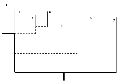
Figure 18: Dendrogram illustration of SIGDISCONT’s unexpected behavior in the presence of significantly extended islands. Cloud number 7 is eliminated from the catalog since it cannot merge with cloud 1 due to discontinuous maxima between them.

Appendix C Inventory of dynamically-motivated environments for M51

The morphology of the grand-design spiral galaxy M51 is ideal for studying the properties of the molecular gas in different galactic environments. Within the PAWS field there are three main regions where the molecular gas is likely subject to distinct physical conditions (see Fig. 2), i.e. within the strong, nearly symmetric spiral arms, the inter-arm region situated upstream and downstream of the spiral arms and the central region, where the gas is influenced by the presence of a central elliptical concentration of old stars in the form of a nuclear bar (Zaritsky et al. 1993). These regions can be further divided into sub-regions, in light of the pattern of star formation (e.g. traced by H${\alpha}$) and gas flows (according to the profile of present-day torques; Meidt et al. 2013) within each.

Specifically, the central region is divided into 2 regions:

• nuclear bar environment (NB): $R_{gal}<23"$, bounded by the bar corotation resonance, inside of which the bar exerts negative torques and drives gas radially inwards

• molecular ring environment (MR): $23"<R_{gal}<35"$ where the influence of the bar and innermost portion of the spiral arms overlap, creating a ring-like accumulation of gas. The ring is sitting where the opposing forces of inner bar and the spiral density-wave cancel out. The high gas surface densities reached at this location result the most prominent star formation in M51.
  

Likewise, we divide the spiral arms region (SA) into three distinct environments according to the direction of gas flows driven in response to the underlying gravitational potential.

• inner density-wave spiral arm environment (DWI): $35"<R_{gal}<55"$ within which gas is driven radially inward by negative spiral-arm torquing. This portion of the spiral arm is characterized by relatively little star formation as traced by H${\alpha}$ and 24 $\mu m$ emission (Schinnerer et al. 2013)

• outer density-wave spiral arm environment (DWO): $55"<R_{gal}<85"$ within which gas is driven radially outward by positive spiral arm torquing. Star formation falls on the convex side of this portion of the spiral arms (Schinnerer et al. 2013)

• material spiral arm environment (MAT): $R_{gal}>85"$ beyond the boundary of positive spiral arm torques associated with the density wave spiral, extending to the edge of the PAWS field (within which there is some indication that the direction of the gas flow is again reversed).
  

The width of the spiral arm environment (and each of its 3 sub-regions) is defined with respect to observed gas kinematics. We determine the zone of enhanced spiral streaming centered around the arm by measuring the (rotational) auto-correlation of azimuthal streaming velocities in the PAWS field (Meidt et al. 2013). We construct azimuthal profiles of the auto correlation signal in a series of radial bins and take the width of the signal at 95% maximum as our measure of the kinematic arm width. In testing, we find that the 95% max-width of the CO-brightness auto correlation profile corresponds well with the width estimated by eye from the morphology of CO brightness (Schinnerer et al. 2013). The average kinematic width along the two arms is centered on the spiral arm ridge located by eye in the PAWS map of CO brightness. Both the location of the ridge and the width are assumed to be symmetric.

This definition of the location and width of the spiral arm ultimately yields the definition of the inter-arm region (IA), which we further divide in to

• downstream of the spiral arms (DNS), or the convex side where the majority of star formation related to the arms is observed in H$\alpha$ or 24 $\mu$m;

• upstream of the spiral arms (UPS), or the concave side basically devoid of significant star formation.

Although inside and outside corotation the gas flow direction should change and hence the definition of up- and down-stream environments, M51 is characterized by a non-trivial dynamical structure composed by several patterns (or potential perturbations) with different pattern speeds e.g (Meidt et al. 2013, Meidt et al. 2008, Vogel et al. 1993, Elmegreen et al. 1989, Tully 1974). Meidt et al. (2013) identified $\Omega_{b}\sim 200$ km s^-1 kpc^-1 at $R_{gal}\sim 20"$ corresponding to the nuclear bar corotation, $\Omega_{p,1}\sim 90$ km s^-1 kpc^-1 at $R_{gal}\sim 55"$ corresponding to the inner spiral arms, $\Omega_{p,2}\sim 55$ km s^-1 kpc^-1 at $R_{gal}\sim 85"$ the transition between density-wave spiral arms and material arms. This suggests that at any radius (within the PAWS FoV) a pattern is inside a corotation resonance of another and thus the expected reversal gas flow for a single pattern is not observed. This interpretation is supported also by the presence of the massive star formation regions along the convex side of the spiral arms only. We therefore designate the convex side of the arms as downstream, and the concave side as upstream, independent of the corotation resonances. These environments are separated at the midpoint of the two spiral arm ridge-lines.

Appendix D Kolmogorov-Smirnov test matrices

The tables presented here list the results of the two-sided Kolmogorov-Smirnov (KS) tests that were carried out to evaluate differences in the cloud property distributions for different M51 environments (see Section 5). To account for measurement errors, we generated random values of a given property within the bootstrap uncertainties reported by CPROPS and we performed the test using the KSTWO procedure of the IDL astrolibrary. The results listed in the tables are median and MAD of p-values obtained through 100 trials. P-values lower than 0.01 show that the cumulative distribution function of the two statistical samples are significantly different and are indicated in bold. Values lower than 0.001 are substituted with $\mathbf{<}0.001$. Differences with moderate statistical significance (up to 0.05) are indicated in italics. Results in the upper right of the matrix are for the highly reliable sample of objects ($S/N>6.5$), while results in the lower left are for the full cloud sample. CPROPS does not provide uncertainties on the peak brightness temperature measurements. We generate these using the $\sigma_{RMS}$ of the noise fluctuations along the line-of-sight where a given GMC peak temperature has been measured.

$\mathbf{T_{max}}$	$\rightarrow$	Highly reliable ($S/N>6.5$)
$\downarrow$	Envir.	NB	MR	DWI	DWO	MAT	DNS	UPS
	NB	x	$\mathbf{0.007\pm 0.002}$	$\mathbf{0.009\pm 0.004}$	$0.126\pm 0.021$	$\mathit{0.049\pm 0.007}$	$\mathbf{<0.001}$	$\mathbf{<0.001}$
	MR	$0.066\pm 0.007$	x	$\mathbf{<0.001}$	$\mathbf{<0.001}$	$\mathbf{0.002\pm 0.001}$	$\mathbf{<0.001}$	$\mathbf{<0.001}$
Full	DWI	$\mathbf{<0.001}$	$\mathbf{<0.001}$	x	$0.093\pm 0.026$	$0.382\pm 0.000$	$\mathit{0.027\pm 0.014}$	$\mathbf{<0.001}$
	DWO	$\mathbf{0.002\pm 0.001}$	$\mathbf{<0.001}$	$0.072\pm 0.008$	x	$0.819\pm 0.024$	$\mathbf{<0.001}$	$\mathbf{<0.001}$
sample	MAT	$\mathbf{<0.001}$	$\mathbf{<0.001}$	$0.171\pm 0.107$	$0.857\pm 0.124$	x	$\mathbf{0.006\pm 0.002}$	$\mathbf{<0.001}$
	DNS	$\mathbf{<0.001}$	$\mathbf{<0.001}$	$\mathit{0.015\pm 0.007}$	$\mathbf{<0.001}$	$\mathbf{0.003\pm 0.001}$	x	$\mathbf{0.008\pm 0.006}$
	UPS	$\mathbf{<0.001}$	$\mathbf{<0.001}$	$\mathbf{0.001\pm 0.001}$	$\mathbf{<0.001}$	$\mathbf{<0.001}$	$\mathbf{<0.001}$	x

$\mathbf{R}$	$\rightarrow$	Highly reliable ($S/N>6.5$)
$\downarrow$	Envir.	NB	MR	DWI	DWO	MAT	DNS	UPS
	NB	x	$0.600\pm 0.098$	$0.296\pm 0.149$	$0.586\pm 0.558$	$0.455\pm 0.427$	$\mathit{0.038\pm 0.056}$	$0.581\pm 0.459$
	MR	$0.797\pm 0.187$	x	$0.603\pm 0.313$	$0.333\pm 0.291$	$0.287\pm 0.226$	$\mathbf{0.005\pm 0.007}$	$0.457\pm 0.315$
Full	DWI	$0.672\pm 0.322$	$0.357\pm 0.433$	x	$0.295\pm 0.308$	$0.384\pm 0.469$	$\mathbf{0.002\pm 0.003}$	$0.357\pm 0.384$
	DWO	$0.202\pm 0.197$	$0.215\pm 0.184$	$0.272\pm 0.156$	x	$0.885\pm 0.114$	$0.125\pm 0.181$	$0.945\pm 0.054$
sample	MAT	$0.279\pm 0.309$	$0.296\pm 0.167$	$0.283\pm 0.198$	$0.983\pm 0.019$	x	$0.535\pm 0.479$	$0.934\pm 0.057$
	DNS	$\mathbf{0.001\pm 0.002}$	$\mathbf{0.002\pm 0.002}$	$\mathbf{0.006\pm 0.009}$	$0.082\pm 0.119$	$0.071\pm 0.093$	x	$0.274\pm 0.202$
	UPS	$0.089\pm 0.130$	$0.083\pm 0.120$	$0.106\pm 0.130$	$0.402\pm 0.348$	$0.432\pm 0.228$	$0.643\pm 0.225$	x

Table 11: Kolmogorov-Smirnov test for Peak temperature (top) and Radius (bottom).

$\mathbf{\sigma_{v}}$	$\rightarrow$	Highly reliable ($S/N>6.5$)
$\downarrow$	Envir.	NB	MR	DWI	DWO	MAT	DNS	UPS
	NB	x	$0.071\pm 0.056$	$0.173\pm 0.065$	$0.734\pm 0.279$	$0.128\pm 0.109$	$\mathbf{<0.001}$	$0.060\pm 0.084$
	MR	$0.231\pm 0.126$	x	$0.545\pm 0.202$	$0.107\pm 0.102$	$\mathbf{0.007\pm 0.009}$	$\mathbf{<0.001}$	$\mathbf{<0.001}$
Full	DWI	$0.486\pm 0.547$	$0.188\pm 0.102$	x	$0.395\pm 0.195$	$0.050\pm 0.045$	$\mathbf{<0.001}$	$\mathbf{0.002\pm 0.002}$
	DWO	$0.595\pm 0.196$	$0.115\pm 0.114$	$0.700\pm 0.135$	x	$0.052\pm 0.053$	$\mathbf{<0.001}$	$\mathbf{0.008\pm 0.011}$
sample	MAT	$\mathbf{0.007\pm 0.010}$	$\mathbf{<0.001}$	$\mathbf{0.002\pm 0.003}$	$\mathbf{<0.001}$	x	$\mathit{0.018\pm 0.024}$	$0.154\pm 0.161$
	DNS	$\mathbf{<0.001}$	$\mathbf{<0.001}$	$\mathbf{<0.001}$	$\mathbf{<0.001}$	$0.069\pm 0.100$	x	$0.175\pm 0.232$
	UPS	$\mathit{0.017\pm 0.026}$	$\mathbf{<0.001}$	$\mathit{0.024\pm 0.025}$	$\mathbf{0.004\pm 0.005}$	$0.247\pm 0.255$	$\mathit{0.022\pm 0.018}$	x

$\mathbf{b/a}$	$\rightarrow$	Highly reliable ($S/N>6.5$)
$\downarrow$	Envir.	NB	MR	DWI	DWO	MAT	DNS	UPS
	NB	x	$0.503\pm 0.133$	$0.981\pm 0.008$	$0.965\pm 0.026$	$0.129\pm 0.029$	$0.227\pm 0.075$	$0.634\pm 0.069$
	MR	$0.606\pm 0.306$	x	$0.382\pm 0.031$	$0.127\pm 0.044$	$0.300\pm 0.092$	$0.503\pm 0.249$	$0.988\pm 0.011$
Full	DWI	$0.808\pm 0.103$	$0.596\pm 0.096$	x	$0.847\pm 0.129$	$0.106\pm 0.073$	$0.191\pm 0.027$	$0.537\pm 0.003$
	DWO	$0.889\pm 0.066$	$0.576\pm 0.100$	$0.903\pm 0.088$	x	$\mathit{0.037\pm 0.018}$	$0.071\pm 0.023$	$0.263\pm 0.045$
sample	MAT	$\mathbf{0.009\pm 0.004}$	$\mathit{0.012\pm 0.013}$	$\mathbf{0.005\pm 0.002}$	$\mathbf{<0.001}$	x	$0.841\pm 0.103$	$0.764\pm 0.160$
	DNS	$\mathit{0.025\pm 0.017}$	$0.108\pm 0.038$	$\mathit{0.037\pm 0.014}$	$\mathit{0.013\pm 0.004}$	$0.409\pm 0.119$	x	$0.973\pm 0.028$
	UPS	$0.130\pm 0.100$	$0.307\pm 0.245$	$0.158\pm 0.153$	$\mathit{0.039\pm 0.045}$	$0.495\pm 0.078$	$0.971\pm 0.032$	x

$\mathbf{\phi}$	$\rightarrow$	Highly reliable ($S/N>6.5$)
$\downarrow$	Envir.	NB	MR	DWI	DWO	MAT	DNS	UPS
	NB	x	$\mathbf{<0.001}$	$\mathbf{<0.001}$	$\mathbf{<0.001}$	$\mathbf{<0.001}$	$\mathbf{<0.001}$	$\mathbf{<0.001}$
	MR	$\mathbf{<0.001}$	x	$\mathbf{<0.001}$	$\mathbf{<0.001}$	$\mathbf{<0.001}$	$\mathbf{<0.001}$	$\mathbf{<0.001}$
Full	DWI	$\mathbf{<0.001}$	$\mathbf{0.001\pm 0.000}$	x	$\mathbf{<0.001}$	$\mathbf{<0.001}$	$\mathbf{<0.001}$	$\mathbf{<0.001}$
	DWO	$\mathbf{<0.001}$	$\mathbf{<0.001}$	$\mathbf{<0.001}$	x	$\mathbf{0.008\pm 0.000}$	$\mathbf{0.003\pm 0.000}$	$\mathbf{0.006\pm 0.000}$
sample	MAT	$\mathbf{<0.001}$	$\mathbf{<0.001}$	$\mathbf{<0.001}$	$\mathbf{<0.001}$	x	$\mathbf{0.001\pm 0.000}$	$0.060\pm 0.000$
	DNS	$\mathbf{<0.001}$	$\mathbf{<0.001}$	$\mathbf{<0.001}$	$\mathbf{<0.001}$	$\mathbf{<0.001}$	x	$0.863\pm 0.000$
	UPS	$\mathbf{<0.001}$	$\mathbf{<0.001}$	$\mathbf{<0.001}$	$\mathbf{<0.001}$	$\mathbf{0.010\pm 0.000}$	$0.547\pm 0.000$	x

Table 12: Kolmogorov-Smirnov test for Velocity dispersion (top), Axis ratio (middle) and Orientation (bottom).

$\mathbf{M_{lum}}$	$\rightarrow$	Highly reliable ($S/N>6.5$)
$\downarrow$	Envir.	NB	MR	DWI	DWO	MAT	DNS	UPS
	NB	x	$\mathit{0.040\pm 0.042}$	$0.286\pm 0.154$	$0.055\pm 0.033$	$0.484\pm 0.387$	$\mathbf{<0.001}$	$\mathbf{0.004\pm 0.006}$
	MR	$0.196\pm 0.126$	x	$0.097\pm 0.106$	$0.564\pm 0.211$	$\mathbf{0.002\pm 0.002}$	$\mathbf{<0.001}$	$\mathbf{<0.001}$
Full	DWI	$\mathit{0.024\pm 0.032}$	$\mathit{0.017\pm 0.018}$	x	$0.237\pm 0.136$	$0.238\pm 0.261$	$\mathbf{0.001\pm 0.002}$	$\mathit{0.017\pm 0.021}$
	DWO	$\mathit{0.044\pm 0.057}$	$0.233\pm 0.089$	$0.257\pm 0.139$	x	$\mathit{0.029\pm 0.031}$	$\mathbf{<0.001}$	$\mathbf{<0.001}$
sample	MAT	$\mathbf{0.002\pm 0.002}$	$\mathbf{<0.001}$	$0.256\pm 0.153$	$\mathit{0.037\pm 0.043}$	x	$\mathit{0.011\pm 0.015}$	$\mathit{0.031\pm 0.040}$
	DNS	$\mathbf{<0.001}$	$\mathbf{<0.001}$	$\mathbf{<0.001}$	$\mathbf{<0.001}$	$\mathbf{0.008\pm 0.011}$	x	$0.364\pm 0.181$
	UPS	$\mathbf{<0.001}$	$\mathbf{<0.001}$	$\mathbf{<0.001}$	$\mathbf{<0.001}$	$\mathit{0.011\pm 0.015}$	$0.547\pm 0.230$	x

$\mathbf{M_{vir}}$	$\rightarrow$	Highly reliable ($S/N>6.5$)
$\downarrow$	Envir.	NB	MR	DWI	DWO	MAT	DNS	UPS
	NB	x	$0.165\pm 0.125$	$\mathit{0.026\pm 0.033}$	$0.548\pm 0.518$	$0.072\pm 0.105$	$\mathbf{<0.001}$	$\mathit{0.036\pm 0.054}$
	MR	$0.397\pm 0.140$	x	$0.418\pm 0.337$	$0.086\pm 0.087$	$\mathbf{<0.001}$	$\mathbf{<0.001}$	$\mathbf{<0.001}$
Full	DWI	$0.142\pm 0.076$	$0.442\pm 0.206$	x	$\mathit{0.019\pm 0.022}$	$\mathbf{<0.001}$	$\mathbf{<0.001}$	$\mathbf{<0.001}$
	DWO	$0.415\pm 0.397$	$\mathit{0.021\pm 0.030}$	$0.089\pm 0.120$	x	$0.069\pm 0.053$	$\mathbf{<0.001}$	$\mathit{0.025\pm 0.014}$
sample	MAT	$\mathbf{0.004\pm 0.006}$	$\mathbf{<0.001}$	$\mathbf{<0.001}$	$\mathit{0.013\pm 0.014}$	x	$0.109\pm 0.064$	$0.343\pm 0.136$
	DNS	$\mathbf{<0.001}$	$\mathbf{<0.001}$	$\mathbf{<0.001}$	$\mathbf{<0.001}$	$0.150\pm 0.140$	x	$0.281\pm 0.196$
	UPS	$0.052\pm 0.076$	$\mathbf{0.004\pm 0.006}$	$\mathbf{0.003\pm 0.004}$	$0.095\pm 0.080$	$0.548\pm 0.140$	$\mathit{0.031\pm 0.032}$	x

$\mathbf{\Sigma_{H2}}$	$\rightarrow$	High reliable ($S/N>6.5$)
$\downarrow$	Envir.	NB	MR	DWI	DWO	MAT	DNS	UPS
	NB	x	$\mathit{0.050\pm 0.073}$	$0.746\pm 0.288$	$0.063\pm 0.081$	$0.623\pm 0.277$	$0.125\pm 0.146$	$0.075\pm 0.099$
	MR	$0.122\pm 0.166$	x	$\mathbf{0.003\pm 0.004}$	$0.115\pm 0.098$	$\mathit{0.049\pm 0.034}$	$\mathbf{<0.001}$	$\mathbf{<0.001}$
Full	DWI	$0.296\pm 0.318$	$\mathbf{<0.001}$	x	$\mathit{0.018\pm 0.026}$	$0.485\pm 0.225$	$0.168\pm 0.115$	$0.073\pm 0.033$
	DWO	$0.355\pm 0.252$	$0.161\pm 0.089$	$\mathbf{0.005\pm 0.007}$	x	$0.192\pm 0.248$	$\mathbf{<0.001}$	$\mathbf{<0.001}$
sample	MAT	$0.523\pm 0.306$	$\mathit{0.026\pm 0.019}$	$0.149\pm 0.095$	$0.109\pm 0.139$	x	$\mathit{0.025\pm 0.018}$	$\mathit{0.042\pm 0.029}$
	DNS	$\mathit{0.041\pm 0.061}$	$\mathbf{<0.001}$	$0.363\pm 0.323$	$\mathbf{<0.001}$	$0.074\pm 0.071$	x	$0.387\pm 0.100$
	UPS	$0.086\pm 0.127$	$\mathbf{<0.001}$	$0.086\pm 0.116$	$\mathbf{<0.001}$	$0.055\pm 0.064$	$0.501\pm 0.285$	x

Table 13: Kolmogorov-Smirnov test for Luminosity mass (top), Virial mass (middle) and Surface density (bottom).

$\mathbf{c}$	$\rightarrow$	Highly reliable ($S/N>6.5$)
$\downarrow$	Envir.	NB	MR	DWI	DWO	MAT	DNS	UPS
	NB	x	$0.172\pm 0.114$	$0.265\pm 0.205$	$0.360\pm 0.120$	$0.495\pm 0.471$	$\mathit{0.013\pm 0.019}$	$0.107\pm 0.133$
	MR	$0.140\pm 0.136$	x	$0.684\pm 0.215$	$0.331\pm 0.185$	$\mathbf{0.006\pm 0.008}$	$\mathbf{<0.001}$	$\mathbf{<0.001}$
Full	DWI	$0.265\pm 0.121$	$0.365\pm 0.235$	x	$0.511\pm 0.174$	$\mathit{0.023\pm 0.030}$	$\mathbf{<0.001}$	$\mathbf{<0.001}$
	DWO	$0.304\pm 0.152$	$0.411\pm 0.232$	$0.909\pm 0.105$	x	$\mathit{0.029\pm 0.033}$	$\mathbf{<0.001}$	$\mathbf{0.009\pm 0.014}$
sample	MAT	$0.424\pm 0.520$	$\mathbf{0.004\pm 0.005}$	$\mathbf{0.009\pm 0.013}$	$\mathit{0.014\pm 0.020}$	x	$0.202\pm 0.115$	$0.311\pm 0.119$
	DNS	$\mathit{0.023\pm 0.033}$	$\mathbf{<0.001}$	$\mathbf{<0.001}$	$\mathbf{<0.001}$	$0.158\pm 0.118$	x	$0.497\pm 0.510$
	UPS	$0.447\pm 0.182$	$\mathit{0.015\pm 0.015}$	$\mathit{0.029\pm 0.032}$	$0.080\pm 0.112$	$0.676\pm 0.149$	$0.103\pm 0.088$	x

$\mathbf{\alpha}$	$\rightarrow$	Highly reliable ($S/N>6.5$)
$\downarrow$	Envir.	NB	MR	DWI	DWO	MAT	DNS	UPS
	NB	x	$0.411\pm 0.122$	$0.362\pm 0.249$	$0.079\pm 0.079$	$0.137\pm 0.077$	$0.070\pm 0.023$	$0.430\pm 0.128$
	MR	$0.791\pm 0.186$	x	$\mathit{0.049\pm 0.039}$	$0.284\pm 0.205$	$0.245\pm 0.266$	$0.304\pm 0.248$	$0.648\pm 0.426$
Full	DWI	$0.196\pm 0.166$	$\mathit{0.025\pm 0.022}$	x	$\mathit{0.023\pm 0.026}$	$\mathit{0.018\pm 0.022}$	$\mathit{0.018\pm 0.017}$	$0.080\pm 0.088$
	DWO	$0.578\pm 0.138$	$0.360\pm 0.133$	$\mathit{0.044\pm 0.031}$	x	$0.063\pm 0.084$	$0.170\pm 0.196$	$0.258\pm 0.224$
sample	MAT	$0.372\pm 0.132$	$0.396\pm 0.309$	$\mathit{0.013\pm 0.013}$	$0.127\pm 0.128$	x	$0.648\pm 0.252$	$0.752\pm 0.291$
	DNS	$0.178\pm 0.228$	$0.217\pm 0.215$	$\mathbf{0.005\pm 0.005}$	$0.339\pm 0.427$	$0.677\pm 0.237$	x	$0.777\pm 0.212$
	UPS	$0.456\pm 0.262$	$0.172\pm 0.089$	$0.425\pm 0.286$	$\mathit{0.026\pm 0.025}$	$\mathit{0.039\pm 0.036}$	$\mathbf{0.009\pm 0.006}$	x

Table 14: Kolmogorov-Smirnov test for Scaling parameter (top) and Virial parameter (bottom).

References

- Aalto et al. (1999) Aalto, S., Hüttemeister, S., Scoville, N. Z., & Thaddeus, P. 1999, ApJ, 522, 165
- Akritas & Bershady (1996) Akritas, M. G., & Bershady, M. A. 1996, ApJ, 470, 706
- Athanassoula (1992) Athanassoula, E. 1992, MNRAS, 259, 345
- Ballesteros-Paredes (2006) Ballesteros-Paredes, J. 2006, MNRAS, 372, 443
- Bell et al. (2007) Bell, T. A., Viti, S., & Williams, D. A. 2007, MNRAS, 378, 983
- Bertoldi & McKee (1992) Bertoldi, F., & McKee, C. F. 1992, ApJ, 395, 140
- Blitz et al. (2007) Blitz, L., Fukui, Y., Kawamura, A., et al. 2007, Protostars and Planets V, 81
- Blitz (1993) Blitz, L. 1993, Protostars and Planets III, 125
- Bohlin et al. (1978) Bohlin, R. C., Savage, B. D., & Drake, J. F. 1978, ApJ, 224, 132
- Bolatto et al. (2008) Bolatto, A. D., Leroy, A. K., Rosolowsky, E., Walter, F., & Blitz, L. 2008, IAU Symposium, 255, 274
- Bergin et al. (2004) Bergin, E. A., Hartmann, L. W., Raymond, J. C., & Ballesteros-Paredes, J. 2004, ApJ, 612, 921
- Bresolin et al. (2004) Bresolin, F., Garnett, D. R., & Kennicutt, R. C., Jr. 2004, ApJ, 615, 228
- Brunt et al. (2003) Brunt, C. M., Heyer, M. H., Vázquez-Semadeni, E., & Pichardo, B. 2003, ApJ, 595, 824
- Casoli & Combes (1981) Casoli, F., & Combes, F. 1981, Academie des Sciences Paris Comptes Rendus Serie B Sciences Physiques, 293, 761
- Ciardullo et al. (2002) Ciardullo, R., Feldmeier, J. J., Jacoby, G. H., et al. 2002, ApJ, 577, 31
- Cowie (1980) Cowie, L. L. 1980, ApJ, 236, 868
- Dame et al. (2001) Dame, T. M., Hartmann, D., & Thaddeus, P. 2001, ApJ, 547, 792
- Dame et al. (1986) Dame, T. M., Ungerechts, H., & Thaddeus, P. 1986, BAAS, 18, 1024
- Dib et al. (2012) Dib, S., Helou, G., Moore, T. J. T., Urquhart, J. S., & Dariush, A. 2012, ApJ, 758, 125
- Dickman (1978) Dickman, R. L. 1978, ApJS, 37, 407
- Dobbs et al. (2006) Dobbs, C. L., Bonnell, I. A., & Pringle, J. E. 2006, MNRAS, 371, 1663
- Dobbs & Bonnell (2007) Dobbs, C. L., & Bonnell, I. A. 2007, MNRAS, 376, 1747
- Dobbs (2008) Dobbs, C. L. 2008, MNRAS, 391, 844
- Dobbs et al. (2011) Dobbs, C. L., Burkert, A., & Pringle, J. E. 2011, MNRAS, 413, 2935
- Dobbs et al. (2012) Dobbs, C. L., Pringle, J. E., & Burkert, A. 2012, MNRAS, 425, 2157
- Dobbs & Pringle (2013) Dobbs, C. L., & Pringle, J. E. 2013, MNRAS, 432, 653
- Donovan Meyer et al. (2013) Donovan Meyer, J., Koda, J., Momose, R., et al. 2013, ApJ, 772, 107
- Eadie et al. (1971) Eadie, W. T., Drijard, D., & James, F. E. 1971, Amsterdam: North-Holland, 1971,
- Egusa et al. (2011) Egusa, F., Koda, J., & Scoville, N. 2011, ApJ, 726, 85
- Elmegreen (1989) Elmegreen, B. G. 1989, ApJ, 338, 178
- Elmegreen (1993) Elmegreen, B. G. 1993, ApJ, 419, L29
- Elmegreen (2000) Elmegreen, B. G. 2000, ApJ, 530, 277
- Elmegreen et al. (1989) Elmegreen, B. G., Elmegreen, D. M., Seiden, P. E., Lowe, S. A., & Lin, C. C. 1989, BAAS, 21, 1128
- Engargiola et al. (2003) Engargiola, G., Plambeck, R. L., Rosolowsky, E., & Blitz, L. 2003, ApJS, 149, 343
- Fukui et al. (2001) Fukui, Y., Mizuno, N., Yamaguchi, R., Mizuno, A., & Onishi, T. 2001, PASJ, 53, L41
- Fukui (2005) Fukui, Y. 2005, The Cool Universe: Observing Cosmic Dawn, 344, 155
- Fukui et al. (2008) Fukui, Y., Kawamura, A., Minamidani, T., et al. 2008, ApJS, 178, 56
- Fukui & Kawamura (2010) Fukui, Y., & Kawamura, A. 2010, ARA&A, 48, 547
- Garcia-Burillo et al. (1993) Garcia-Burillo, S., Guelin, M., & Cernicharo, J. 1993, A&A, 274, 123
- Garcia-Burillo et al. (1993) Garcia-Burillo, S., Combes, F., & Gerin, M. 1993, A&A, 274, 148
- Glover & Clark (2012) Glover, S. C. O., & Clark, P. C. 2012, MNRAS, 426, 377
- Glover & Mac Low (2007) Glover, S. C. O., & Mac Low, M.-M. 2007, ApJS, 169, 239
- Glover & Mac Low (2007) Glover, S. C. O., & Mac Low, M.-M. 2007, ApJ, 659, 1317
- Gratier et al. (2012) Gratier, P., Braine, J., Rodriguez-Fernandez, N. J., et al. 2012, A&A, 542, A108
- Guelin et al. (1995) Guelin, M., Zylka, R., Mezger, P. G., Haslam, C. G. T., & Kreysa, E. 1995, A&A, 298, L29
- Hagiwara (2007) Hagiwara, Y. 2007, AJ, 133, 1176
- Heithausen et al. (1998) Heithausen, A., Bensch, F., Stutzki, J., Falgarone, E., & Panis, J. F. 1998, A&A, 331, L65
- Heitsch et al. (2008) Heitsch, F., Hartmann, L. W., & Burkert, A. 2008, ApJ, 683, 786
- Heitsch et al. (2009) Heitsch, F., Stone, J. M., & Hartmann, L. W. 2009, ApJ, 695, 248
- Helfer et al. (2003) Helfer, T. T., Thornley, M. D., Regan, M. W., et al. 2003, ApJS, 145, 259
- Heyer et al. (2001) Heyer, M. H., Carpenter, J. M., & Snell, R. L. 2001, ApJ, 551, 85
- Heyer et al. (2009) Heyer, M., Krawczyk, C., Duval, J., & Jackson, J. M. 2009, ApJ, 699, 1092
- Hirota et al. (2011) Hirota, A., Kuno, N., Sato, N., et al. 2011, ApJ, 737, 40
- Hitschfeld et al. (2009) Hitschfeld, M., Kramer, C., Schuster, K. F., Garcia-Burillo, S., & Stutzki, J. 2009, A&A, 495, 795
- Hollenbach & Tielens (1999) Hollenbach, D. J., & Tielens, A. G. G. M. 1999, Reviews of Modern Physics, 71, 173
- Hopkins (2012) Hopkins, P. F. 2012, MNRAS, 423, 2016
- Hughes et al. (2010) Hughes, A., Wong, T., Ott, J., et al. 2010, MNRAS, 406, 2065
- Hughes et al. (2013) Hughes, A., Meidt, S. E., Colombo, D., et al. 2013, arXiv:1309.3453
- Israel et al. (2006) Israel, F. P., Tilanus, R. P. J., & Baas, F. 2006, A&A, 445, 907
- Jog (2013) Jog, C. J. 2013, MNRAS, 434, L56
- Kaufman et al. (1999) Kaufman, M. J., Wolfire, M. G., Hollenbach, D. J., & Luhman, M. L. 1999, ApJ, 527, 795
- Kim et al. (2001) Kim, J., Ryu, D., & Jones, T. W. 2001, ApJ, 557, 464
- Kim et al. (2003) Kim, W.-T., Ostriker, E. C., & Stone, J. M. 2003, ApJ, 599, 1157
- Koda et al. (2009) Koda, J., Scoville, N., Sawada, T., et al. 2009, ApJ, 700, L132
- Koyama & Ostriker (2009) Koyama, H., & Ostriker, E. C. 2009, ApJ, 693, 1346
- Kramer et al. (1998) Kramer, C., Stutzki, J., Rohrig, R., & Corneliussen, U. 1998, A&A, 329, 249
- Kritsuk & Norman (2011) Kritsuk, A. G., & Norman, M. L. 2011, arXiv:1111.2827
- Kuno et al. (1995) Kuno, N., Nakai, N., Handa, T., & Sofue, Y. 1995, PASJ, 47, 745
- Kuno & Nakai (1997) Kuno, N., & Nakai, N. 1997, PASJ, 49, 279
- Kwan (1979) Kwan, J. 1979, ApJ, 229, 567
- Kwan & Valdes (1983) Kwan, J., & Valdes, F. 1983, ApJ, 271, 604
- Kwan & Valdes (1987) Kwan, J., & Valdes, F. 1987, ApJ, 315, 92
- Larson (1981) Larson, R. B. 1981, MNRAS, 194, 809
- La Vigne et al. (2006) La Vigne, M. A., Vogel, S. N., & Ostriker, E. C. 2006, ApJ, 650, 818
- Leroy et al. (2006) Leroy, A., Bolatto, A., Walter, F., & Blitz, L. 2006, ApJ, 643, 825
- Leroy et al. (2008) Leroy, A. K., Walter, F., Brinks, E., et al. 2008, AJ, 136, 2782
- Leroy et al. (2011) Leroy, A. K., Bolatto, A., Gordon, K., et al. 2011, ApJ, 737, 12
- Leroy et al. (2012) Leroy, A. K., Bigiel, F., de Blok, W. J. G., et al. 2012, AJ, 144, 3
- Lo et al. (1987) Lo, K. Y., Ball, R., Masson, C. R., et al. 1987, ApJ, 317, L63
- Maddox et al. (2007) Maddox, L. A., Cowan, J. J., Kilgard, R. E., Schinnerer, E., & Stockdale, C. J. 2007, AJ, 133, 2559
- McKee & Ostriker (2007) McKee, C. F., & Ostriker, E. C. 2007, ARA&A, 45, 565
- Meidt et al. (2008) Meidt, S. E., Rand, R. J., Merrifield, M. R., Shetty, R., & Vogel, S. N. 2008, ApJ, 688, 224
- Meidt et al. (2013) Meidt, S. E., Schinnerer, E., Garcia-Burillo, S., et al. 2013, arXiv:1304.7910
- Mentuch Cooper et al. (2012) Mentuch Cooper, E., Wilson, C. D., Foyle, K., et al. 2012, ApJ, 755, 165
- Mizuno et al. (2006) Mizuno, N., Muller, E., Maeda, H., et al. 2006, ApJ, 643, L107
- Moustakas et al. (2010) Moustakas, J., Kennicutt, R. C., Jr., Tremonti, C. A., et al. 2010, ApJS, 190, 233
- Muñoz-Mateos et al. (2011) Muñoz-Mateos, J. C., Boissier, S., Gil de Paz, A., et al. 2011, ApJ, 731, 10
- Nakai et al. (1994) Nakai, N., Kuno, N., Handa, T., & Sofue, Y. 1994, PASJ, 46, 527
- Patrikeev et al. (2006) Patrikeev, I., Fletcher, A., Stepanov, R., et al. 2006, A&A, 458, 441
- Pety et al. (2013) Pety, J., Schinnerer, E., Leroy, A. K., et al. 2013, arXiv:1304.1396
- Pringle et al. (2001) Pringle, J. E., Allen, R. J., & Lubow, S. H. 2001, MNRAS, 327, 663
- Putman et al. (2012) Putman, M. E., Peek, J. E. G., & Joung, M. R. 2012, ARA&A, 50, 491
- Rand & Kulkarni (1990) Rand, R. J., & Kulkarni, S. R. 1990, NASA Conference Publication, 3084, 293
- Rebolledo et al. (2012) Rebolledo, D., Wong, T., Leroy, A., Koda, J., & Donovan Meyer, J. 2012, ApJ, 757, 155
- Rosolowsky & Leroy (2006) Rosolowsky, E., & Leroy, A. 2006, PASP, 118, 590
- Rosolowsky (2005) Rosolowsky, E. 2005, PASP, 117, 1403
- Rosolowsky & Blitz (2005) Rosolowsky, E., & Blitz, L. 2005, ApJ, 623, 826
- Rosolowsky (2007) Rosolowsky, E. 2007, ApJ, 654, 240
- Sanders et al. (1985) Sanders, D. B., Scoville, N. Z., & Solomon, P. M. 1985, ApJ, 289, 373
- Sawada et al. (2012) Sawada, T., Hasegawa, T., & Koda, J. 2012, ApJ, 759, L26
- Schiminovich et al. (2007) Schiminovich, D., Wyder, T. K., Martin, D. C., et al. 2007, ApJS, 173, 315
- Schinnerer et al. (2010) Schinnerer, E., Weiß, A., Aalto, S., & Scoville, N. Z. 2010, ApJ, 719, 1588
- Schinnerer et al. (2013) Schinnerer, E., Meidt, S. E., Pety, J., et al. 2013, arXiv:1304.1801
- Schuster et al. (2007) Schuster, K. F., Kramer, C., Hitschfeld, M., Garcia-Burillo, S., & Mookerjea, B. 2007, A&A, 461, 143
- Schwarz (1984) Schwarz, M. P. 1984, MNRAS, 209, 93
- Scoville et al. (1987) Scoville, N. Z., Yun, M. S., Sanders, D. B., Clemens, D. P., & Waller, W. H. 1987, ApJS, 63, 821
- Sheth et al. (2002) Sheth, K., Vogel, S. N., Teuben, P. J., et al. 2002, Disks of Galaxies: Kinematics, Dynamics and Peturbations, 275, 267
- Sheth et al. (2008) Sheth, K., Vogel, S. N., Wilson, C. D., & Dame, T. M. 2008, ApJ, 675, 330
- Shetty & Ostriker (2006) Shetty, R., & Ostriker, E. C. 2006, ApJ, 647, 997
- Shetty et al. (2007) Shetty, R., Vogel, S. N., Ostriker, E. C., & Teuben, P. J. 2007, ApJ, 665, 1138
- Simon et al. (2001) Simon, R., Jackson, J. M., Clemens, D. P., Bania, T. M., & Heyer, M. H. 2001, ApJ, 551, 747
- Solomon et al. (1979) Solomon, P. M., Sanders, D. B., & Scoville, N. Z. 1979, ApJ, 232, L89
- Solomon et al. (1987) Solomon, P. M., Rivolo, A. R., Barrett, J., & Yahil, A. 1987, ApJ, 319, 730
- Sorai et al. (2001) Sorai, K., Hasegawa, T., Booth, R. S., et al. 2001, ApJ, 551, 794
- Spearman C (1904) . ”The proof and measurement of association between two things”. Amer. J. Psychol. 15: 72–101
- Stark & Lee (2006) Stark, A. A., & Lee, Y. 2006, ApJ, 641, L113
- Tan et al. (2011) Tan, Q.-H., Gao, Y., Zhang, Z.-Y., & Xia, X.-Y. 2011, Research in Astronomy and Astrophysics, 11, 787
- Tasker & Tan (2009) Tasker, E. J., & Tan, J. C. 2009, ApJ, 700, 358
- Tomisaka (1986) Tomisaka, K. 1986, PASJ, 38, 95
- Tully (1974) Tully, R. B. 1974, ApJS, 27, 449
- Tukey (1977) Tukey, J. W. 1977, Addison-Wesley Series in Behavioral Science: Quantitative Methods, Reading, Mass.: Addison-Wesley, 1977,
- Vogel et al. (1988) Vogel, S. N., Kulkarni, S. R., Scoville, N. Z., & Hester, J. 1988, Molecular Clouds, Milky-Way and External Galaxies, 315, 437
- Vogel et al. (1993) Vogel, S. N., Rand, R. J., Gruendl, R. A., & Teuben, P. J. 1993, PASP, 105, 666
- Williams & McKee (1997) Williams, J. P., & McKee, C. F. 1997, ApJ, 476, 166
- Wong et al. (2011) Wong, T., Hughes, A., Ott, J., et al. 2011, ApJS, 197, 16
- Young & Scoville (1991) Young, J. S., & Scoville, N. Z. 1991, ARA&A, 29, 581
- Zaritsky et al. (1993) Zaritsky, D., Rix, H.-W., & Rieke, M. 1993, Nature, 364, 313