CO isotopologues in the Perseus Molecular Cloud Complex: the $X$-factor and regional variations

Abstract

The COMPLETE Survey of Star-Forming regions offers an unusually comprehensive and diverse set of measurements of the distribution and temperature of dust and gas in molecular clouds, and in this paper we use those data to find new calibrations of the “X-factor” and the ¹³CO abundance within Perseus. To carry out our analysis, we: 1) apply the NICER (Near-Infrared Color Excess Method Revisited) algorithm to 2MASS data to measure dust extinction; 2) use dust temperatures derived from re-processed IRAS data; and 3) make use of the ¹²CO and ¹³CO (1-0) transition maps gathered by COMPLETE to measure gas distribution and temperature. Here, we divide Perseus into six sub-regions, using groupings in a plot of dust temperature as a function of LSR velocity. The standard $X$ factor, $X\equiv N({\rm H_{2}})/W({\rm{}^{12}CO})$, is derived both for the whole Perseus Complex and for each of the six sub-regions with values consistent with previous estimates. However, the $X$ factor is heavily affected by the saturation of the emission above $A_{V}$$\sim$4 mag, and variations are found between regions. We derive linear fits to relate $W({\rm{}^{12}CO})$ and $A_{V}$ using only points below 4 mag of extinction. This linear fit yields a better estimation of the $A_{V}$ than the $X$ factor. We derive linear relations of $W({\rm{}^{13}CO}),N({\rm{}^{13}CO})$ and $W({\rm C^{18}O})$ with $A_{V}$. In general, the extinction threshold above which ¹³CO (1-0) and C¹⁸O (1-0) are detected is about 1 mag larger than previous estimates, so that a more efficient shielding is needed for the formation of CO than previously thought. The fractional abundances (w.r.t. H₂ molecules) are in agreement with previous works. The (1-0) lines of ¹²CO and ¹³CO saturate above 4 and 5 mag, respectively, whereas C¹⁸O (1-0) never saturates in the whole $A_{V}$ range probed by our study (up to 10 mag). Approximately 60% of the positions with ¹²CO (1-0) emission have sub-thermally excited lines, and almost all positions have ¹²CO (1-0) excitation temperatures below the dust temperature. We compare our data with PDR models using the Meudon code, finding that ¹²CO (1-0) and ¹³CO (1-0) emission can be explained by these uniform slab models with densities ranging between about $10^{3}$ and $10^{4}~{}{\rm cm^{-3}}$. In general, local variations in the volume density and non-thermal motions (linked to different star formation activity) can explain the observations. Higher densities are needed to reproduce CO data toward active star forming sites, such as NGC 1333, where the larger internal motions driven by the young protostars allow more photons from the embedded high density cores to escape the cloud. In the most quiescent region, B5, the ¹²CO and ¹³CO emission appears to arise from an almost uniform thin layer of molecular material at densities around $10^{4}~{}{\rm cm^{-3}}$, and the integrated intensities of the two CO isotopologues are the lowest in the whole complex.

1 Introduction

Although H₂ is the most abundant molecule in the interstellar medium (by about four orders of magnitude), it cannot be used as a tracer of the physical conditions in a molecular cloud. In fact, being a homonuclear species, H₂ does not have an electric dipole moment and even the lowest (electric quadrupole) rotational transitions require temperatures and densities well above those found in typical molecular clouds. The next most abundant molecule is ¹²CO, and since its discovery by Wilson et al. (1970) it has been considered the best tracer of H₂  and the total mass of molecular clouds (e.g. Combes, 1991). Because of its relatively large abundance and excitation properties, the ¹²CO (1-0) line is typically optically thick in molecular clouds, so that rarer CO isotopomers (in particular ¹³CO) have also been used to trace the cloud mass in the most opaque regions. However, previous attempts to derive cloud masses from the thinner isotopomers present a large scatter (factor of 10), indicating that ¹³CO line strength is not an entirely straightforward indicator of gas column. In particular, the following points should be taken into account to derive less uncertain conversions: 1) preferential photodissociation of ¹³CO at low optical extinctions, $A_{V}$; 2) active chemical fractionation in the presence of ¹³C⁺ ions, enhancing the relative abundance of ¹³CO in cold gas (Watson, 1977); and 3) variations in the ¹²CO/¹³CO abundance ratio across the Galaxy.

The conversion between ¹²CO (1-0) integrated intensity ($W({\rm{}^{12}CO})$) and H₂ column density ($N({\rm H_{2}})$) is usually made using the so-called “X-factor,” defined as

$$X\equiv\frac{N({\rm H_{2}})}{W({\rm{}^{12}CO})}~{}.$$ (1)

In order to calibrate this ratio, one needs to measure the column of H₂  which is difficult to do reliably.

One method to derive this ratio uses only the ¹²CO emission and the assumption that molecular clouds are close to virial equilibrium. Solomon et al. (1987) found a tight relation between the molecular cloud virial mass and the ¹²CO luminosity ($M_{\rm VT}=39(L_{\rm CO})^{0.81}$). This relation enabled them to derive a ratio of ${\bf 3.0}\times 10^{20}~{}{\rm cm^{-2}\,K^{-1}\,km^{-1}\,s}$ for the median mass of the sample ($10^{5}~{}M_{\odot}$). In this case, the main source of uncertainty is the assumption of virial equilibrium for the molecular clouds.

Another method uses the generation of gamma rays by the collision of cosmic rays with H and H₂. The H₂ abundance is calculated using (assumed optically thin) 21-cm observations of H I and gamma ray observations in concert. Bloemen et al. (1986) using COS-B data derived a value of $({\bf 2.8}\pm 0.4)\times 10^{20}~{}{\rm cm^{-2}\,K^{-1}\,km^{-1}\,s}$ for the X factor, while Strong & Mattox (1996) derived $({\bf 1.9}\pm 0.2)\times 10^{20}~{}{\rm cm^{-2}\,K^{-1}\,km^{-1}\,s}$ using the EGRET data. Uncertainties in gamma-ray-derived estimates of the X-factor stem from coarse resolution (0.5° and 0.2° for COS-B and EGRET, respectively) and from the assumption that there are no point sources of gamma rays.

An alternative method to derive the column density of H₂ makes use of the IRAS 100 $\mu$m data to estimate the total column density of dust, which can then be used, assuming a constant dust-to-gas ratio (=0.01, value adopted also here), to estimate the total column density of Hydrogen ($N({\rm H})=N(\textrm{{H~{}I}})+2N({\rm H_{2}})$) and derive the conversion factor $X$. Using this method Dame et al. (2001) derived a value of $({\bf 1.8}\pm 0.3)\times 10^{20}~{}{\rm cm^{-2}\,K^{-1}\,km^{-1}\,s}$ for the disk of the Milky Way, while de Vries et al. (1987) derived $({\bf 0.5}\pm 0.3)\times 10^{20}~{}{\rm cm^{-2}\,K^{-1}\,km^{-1}\,s}$ for the high-latitude far-infrared “cirrus” clouds in Ursa Major. Frerking et al. (1982) find no correlation at all between $W({\rm{}^{12}CO})$ and $N({\rm H_{2}})$ in Taurus (where the ¹²CO (1-0) integrated intensity is roughly constant above 2 mag of visual extinction) while in $\rho$-Ophiuchus they derive $({\bf 1.8}\pm 0.1)\times 10^{20}~{}{\rm cm^{-2}\,K^{-1}\,km^{-1}\,s}$.

More recently, Lombardi et al. (2006) studied the Pipe Cloud using an extinction map derived using the Near Infrared Color Excess Revisited (NICER) technique on 2MASS and ¹²CO (1-0) data. They derived an $X$ factor of $({\bf 2.91}\pm 0.05)\times 10^{20}~{}{\rm cm^{-2}\,K^{-1}\,km^{-1}\,s}$, similar to what is found in cloud core regions and dark nebulae (see compilation by Young & Scoville, 1982). However, the factor derived by Lombardi et al. (2006) includes a correction for Helium and uses the non-standard expression $N({\rm H})=N(\textrm{{H~{}I}})+N({\rm H_{2}})$, while using the standard definition of $N({\rm H})=N(\textrm{{H~{}I}})+2N({\rm H_{2}})$ they would derive $({\bf 1.06}\pm 0.02)\times 10^{20}~{}{\rm cm^{-2}\,K^{-1}\,km^{-1}\,s}$.

Frerking et al. (1982) studied the relation between visual extinction and ¹³CO data, and found that the number of H₂ molecules per ¹³CO molecule, [H₂/¹³CO], is ${\bf 3.7}\times 10^{5}$ in Taurus and ${\bf 3.5}\times 10^{5}$ in Ophiuchus, with extinction thresholds (below which no ¹³CO is detected) of ${\bf 1.0}$ and ${\bf 1.6}$ mag, respectively. To make these estimates, Frerking et al. (1982) derived pencil-beam extinctions along the line of sight towards a handful of positions with background stars, by using near-infrared (NIR) spectroscopy from Elias (1978) to estimate the spectral type and derive the extinction. However, pencil beam observations do not trace the same material probed by the molecular line emission observations, and this can introduce large uncertainties. In fact, Arce & Goodman (1999) compared spectroscopically-determined extinction and IRAS-derived extinction in a stripe through Taurus, finding a 1-$\sigma$ dispersion of 15% when the extinctions are compared between $0.9<A_{V}<3.0$ mag. This unavoidable dispersion is likely to affect previous column density derivations, such as Frerking et al. (1982), as well.

Previous studies of the ¹³CO abundance have also been carried out specifically in the portions of the Perseus Molecular Cloud Complex we study here. Bachiller & Cernicharo (1986) used an extinction map derived from star counting on the Palomar Observatory Sky Survey (Cernicharo & Bachiller, 1984). The angular resolution of their extinction map is $2.5\arcmin$, which is smoothed to $5\arcmin$ resolution for comparison with the $4.4\arcmin$ resolution of their ¹³CO data, from which they derive an [H₂/¹³CO] abundance and threshold extinction of ${\bf 3.8}\times 10^{5}$ and ${\bf 0.8}$ mag, respectively. Langer et al. (1989) compare ¹³CO  data of $2\arcmin$ resolution with the extinction map derived by Cernicharo & Bachiller (1984), obtaining [H₂/¹³CO]$={\bf 3.6}\times 10^{5}$ and an extinction threshold of ${\bf 0.5}$ mag. However, this study was done only in the B5 region. A summary of earlier measurements of the X-factor and ¹³CO abundances can be found in §§ 6.2 and 6.3.

The main disadvantage of previous calibrations done on Perseus is that they use optically-based star counting to create extinction maps of regions with high visual extinction (Bachiller & Cernicharo, 1986; Langer et al., 1989). For Ophiuchus, Schnee et al. (2005) find that the extinction derived using optical star counting (Cambrésy, 1999) is systematically underestimated by $\sim 0.8$ mag in comparison with near-IR-based extinction mapping. The offset (and resulting inaccuracy) is caused by the difficulty in fixing the zero-point extinction level – in such a high extinction region – in the optical star counting extinction map. In addition, the derived $A_{V}$ from optical star counting in Perseus does not have a large dynamic range ($A_{V}<5~{}\rm{mag}$), while the NICER extinction map used in our work is accurate up to $10~{}\rm{mag}$ with small errors ($\sigma_{A_{V}}<0.35~{}\rm{mag}$; see Ridge et al., 2006a).

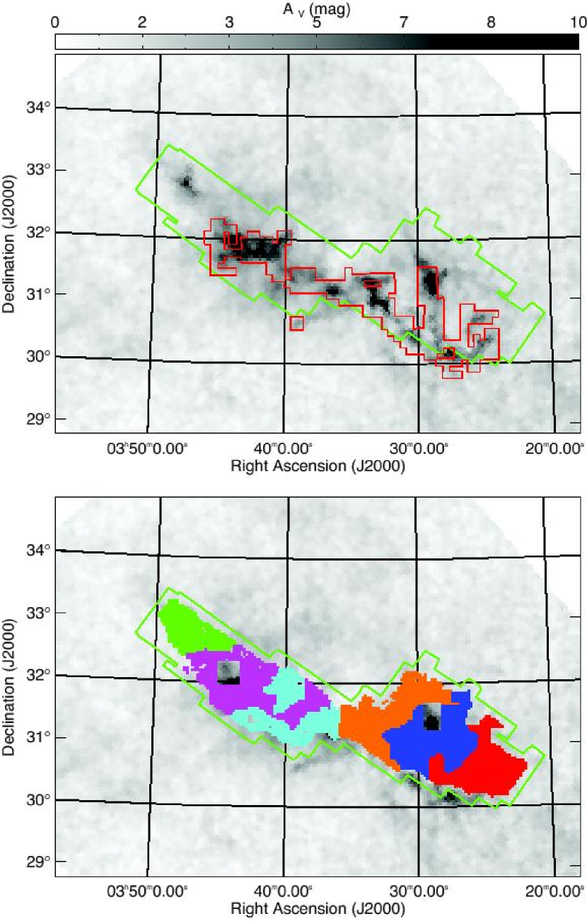
Figure 3: (Top) The extinction map derived using NICER. The green border is the region observed in ¹²CO  and ¹³CO (1-0) by COMPLETE, while the red border is the region observed in C¹⁸O (1-0) by Hatchell & van der Tak (2003). (Bottom) The re-gridded molecular data that fulfil the requirements detailed in § 3 are shown as boxes. Each of the defined regions are presented in a different color. B5 is green, IC 348 is magenta, the Shell is cyan, B1 is orange, NGC 1333 is blue and Westend is red.

The B5 region in Perseus is special, in that it has been the subject of an unusually high number of studies seeking to understand its basic physical properties. As shown in Figure 3, B5 is somewhat isolated from the rest of Perseus, and it is only forming a very small number of stars, making it an obviously good choice for detailed study. Young et al. (1982) used a LVG model to derive an average density of $1.7\times 10^{3}~{}{\rm cm^{-3}}$ and kinetic temperatures $\sim 10-15$ K, but only for some stripes in the cloud. Bensch (2006) used ¹²CO and ¹³CO maps with C I pointing observations of 12 positions in a North-South stripe from the central B5 region to model the emission with a PDR code. From this analysis he derives average densities $\sim 3\times 10^{3}-3\times 10^{4}~{}{\rm cm^{-3}}$.

The COMPLETE dataset offers the unique opportunity to study the emission of various CO isotopologues across the whole Perseus complex with unprecedented sensitivity and spatial resolution. In the present paper, COMPLETE data are analysed in detail to measure the ¹²CO excitation, the ¹³CO abundance and the $X$ factor across the complex and study their variations. The observed changes in the measured quantities are then related to local properties of the gas and dust. Using PDR codes, we find that local variations in the volume density and non-thermal motions (linked to different star formation activity) can explain the observations.

The extinction map, molecular and IRAS data used in this paper are presented in Sect. 2. The data selection is discussed in Sect. 3. The six regions in which the Perseus Molecular Cloud Complex is divided are identified in Sect. 4. Section 5 contains the analysis of the data, including the ¹³CO column density determination and the curve of growth. Results can be found in Sect. 6. The comparison between observations and PDR models is in Sec. 7 and conclusions are listed in Sect. 8.

2 Data

2.1 Extinction Map

We use the Near-Infrared Color Excess Method Revisited (NICER) technique (Lombardi & Alves, 2001) on the Two Micron All Sky Survey (2MASS) point source catalog to calculate K-band extinctions. To derive $A_{V}$, we use the relation $A_{K}=0.112~{}A_{V}$ (Rieke & Lebofsky, 1985). The resulting extinction map has a fixed resolution of $5\arcmin$, and the pixel scale is $2.5\arcmin$. The total size of the map is $9\arcdeg\times 12\arcdeg$ and is presented in Ridge et al. (2006a) (see Alves et al., 2007, for more details).

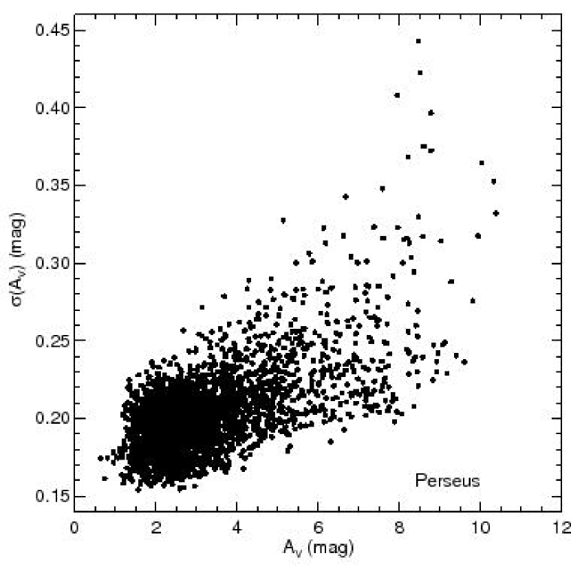
Figure 1: Error in the Perseus extinction map derived with NICER at each pixel versus the corresponding $A_{V}$. Only the pixels used in this study are displayed here.

Figure 1 shows the estimated error (uncertainty) in the derived $A_{V}$ for all the points in the extinction map used in this study. The uncertainties are correlated with the extinction values because more stars per pixel allow for a more accurate measure of extinction. Nevertheless, the linear slope in Figure 1 is smaller than $0.01$, so that the fractional uncertainty in any pixel’s extinction measure remains quite small compared to its value. The median of the error for all of Perseus using NICER on 2MASS data is $0.2$ mag, while in the case of the extinction map derived by Cernicharo & Bachiller (1984) and used in Bachiller & Cernicharo (1986); Langer et al. (1989) the typical error is $\sim 0.5~{}\rm{mag}$.

While the improved accuracy offered by our new maps is significant, the increased dynamic range is even more critical to our analysis. The NICER extinction map of Perseus is accurate up to $A_{V}=10~{}\rm{mag}$, while the extinction map derived using star counting by Cernicharo & Bachiller (1984) dies out above $\sim 4-5~{}\rm{mag}$ of visual extinction.

2.2 Molecular Data

We use the line maps of the COMPLETE Survey (Ridge et al., 2006a) to estimate ¹²CO (1-0) and ¹³CO (1-0) column densities. Both lines were observed simultaneously using the FCRAO telescope. The line maps cover an area of $\sim 6.25\arcdeg\times 3\arcdeg$ with a $46\arcsec$ beam in a $23\arcsec$ grid, and the positions included in our analysis are shown in Figure 3. We correct the ¹²CO (1-0) and ¹³CO (1-0) maps for a main-beam efficiency assumed to be $0.45$ and $0.49$, respectively (http://www.astro.umass.edu/$∼$fcrao/). The flux calibration uncertainty is assumed to be 15% (Mark Heyer, private communication).

In comparing the ¹²CO integrated intensity presented in Dame et al. (2001) with the integrated intensity of our data smoothed to match the $1/8\,\arcdeg$ beam resolution, we find the COMPLETE data and Dame’s measurements to be well fitted by a linear relation of slope $0.9\pm 0.1$ and off-set $-2\pm 1~{}{\rm K\,km\,s^{-1}}$. We also compare the COMPLETE ¹³CO integrated intensity with data from Bell Labs (Padoan et al., 1999), after smoothing our data to the 100$\arcsec$ resolution and 1$\arcmin$ grid of Bell Labs data. These data are fitted by a linear relation of slope $0.986\pm 0.003$ and off-set $-0.53\pm 0.01~{}{\rm K\,km\,s^{-1}}$, where the small deviation from the $1:1$ relation is most probably due to a small misalignment found between the images.

In addition, we use the C¹⁸O (1-0) data-cube presented by Hatchell & van der Tak (2003) (and converted into FITS using CLASS90; Hily-Blant et al., 2005-1), taken with FCRAO but with a smaller coverage and lower signal to noise.

We convolve all data-cubes with a Gaussian beam to obtain the same $5\arcmin$ resolution as the NICER map, and then re-grid them to the extinction map grid of $2.5\arcmin$.

2.3 Column Density and Dust Temperature from IRAS

To estimate column density accurately from far-infrared (thermal) flux, one needs to also measure or calculate a temperature. Normally, this is accomplished by making measurements at two separated far-IR wavelengths, making assumptions about dust emissivity, and then calculating two “unknowns” (column density and temperature) from the two measurements of flux. In the happy case where extinction mapping offers an independent measure of column density over a wide region, the conversion of FIR flux ratios to column density and temperature can be optimized so as to minimize point-to-point differences in comparisons of extinction- and emission-derived column density. The column densities and temperatures derived from dust emission that we use in this paper and in Goodman et al. (2007) come from the work of Schnee et al. (2005), who re-calibrated IRAS-based maps by using the 2MASS/NICER extinction maps discussed above to constrain the column density conversions.

The “IRAS” data used in Schnee et al. (2005) come from the the IRIS (Improved Reprocessing of the IRAS Survey; Miville-Deschênes & Lagache, 2005) flux maps at 60 and 100 µm. The IRIS data have better zodiacal light subtraction, calibration and zero level determinations, and destriping than the earlier ISSA IRAS survey release.

There are two important caveats to apply to the FIR-based column density and temperature measurements we use here (applicable to previous work as well). First, the column densities are only optimized to reduce scatter in a global (Perseus-wide) comparison of dust extinction and emission measures of column density – they are still calculated based on the measured FIR fluxes at each point, and are thus not constrained to be identical to the 2MASS/NICER values. Second, the dust temperatures derived by this method are uncertain due to: 1) unavoidable line-of-sight temperature variations, which cause increased scatter in comparisons with extinction-based measures and also cause a bias toward slightly higher temperatures (see Schnee et al., 2006); and 2) the effect of emission from transiently heated Very Small Grains (see Schnee et al., 2008). That said, the column density and temperature estimates based on Schnee et al. (2005) and used in this paper do represent a dramatic improvement.

3 Data Editing for Analysis

The total number of pixels with data in all maps is 3765. But in order to have high-quality data in every pixel of every map used in our analysis, we trim our maps to exclude particular positions where any data are not reliable. The procedure used in data editing is described in this Section.

3.1 Extinction Map

Regions with both high stellar density and high extinction are typically associated with embedded populations of young stellar objects (YSOs). Thus, in creating extinction maps, including these regions, it would be foolish to assume that stars are background to the cloud and have “typical” near-IR colors. Among YSOs, the more evolved objects observable in J, H, and K bands could in principle still be used to measure the extinction, but the fact that they are not background objects still produces an underestimation of the extinction. This affects the precision of the method much more than the non-stellar IR colors (infrared excess) of YSOs. Therefore, we exclude all the regions with a stellar density larger than $10$ stars per pixel from our analysis. This criterion removes 34 pixels from our maps. In addition to this editing, we exclude a box around each of the two main clusters in Perseus: IC348 and NGC1333, removing another 158 pixels from our data, as is evident in Figure 3 (see Table 1).

3.2 Molecular Transitions

To remain in the analysis, lines must have positive integrated intensities in both ¹²CO and ¹³CO and peak brightness temperatures of at least 10 and 5 times the RMS noise for ¹²CO and ¹³CO respectively.

Since ¹²CO is more abundant than ¹³CO, and self-shielding is more effective for the ¹²CO (1-0) transition than for the ¹³CO (1-0) transition, ¹²CO emission is always more extended than ¹³CO, both spatially and kinematically. In addition, ¹²CO lines are more affected (broadened) by outflows and are optically-thicker than ¹³CO. Thus, line-widths for ¹²CO, $\sigma({\rm{}^{12}CO})$, should always be larger than those of ¹³CO, $\sigma({\rm{}^{13}CO})$. As a result, we keep only positions with

$$\sigma({\rm{}^{12}CO})>0.8\,\sigma({\rm{}^{13}CO})~{},$$

where the 0.8 factor has been chosen to take into account the uncertainties in the line-width determination. The line-widths and central velocities of the spectra are obtained through Gaussian fits. This filtering accounts for only 72 out of the 324 pixels edited out in this study.

3.3 Final Data Set

The result of our editing leaves us with 3400 pixels (shown in Figure 3, see § 4 for details on color coding), out of an original 3724 pixels with ¹³CO detections. Note that our pixels are $2\times$ oversampled (see § 2.2), so that 3400 pixels amounts to 3400/4 independent measures.

4 Region Identification

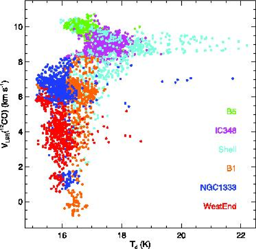
Figure 2: Central velocity compared with the dust temperature. Perseus is divided into six regions that are defined mainly in the space of physical parameters. This separation allows a better understanding of the cloud.

In trying to study Perseus as one object, it became apparent that much of the scatter in both the X-factor and in ¹³CO abundance is caused by region-to-region variations (see §§ 6.2 and 6.3). So, we have divided the Perseus Molecular Cloud Complex into six regions with the help of several plots comparing different parameters (e.g. ¹²CO line-width, ¹²CO LSR velocity, dust and excitation temperature). Figure 2 is an example of such plots, showing the ¹²CO velocity, $V_{LSR}$(¹²CO) (the $V_{LSR}$ of ¹²CO and ¹³CO are very similar) as a function of dust temperature, $T_{d}$, for all the Perseus data. In this way, we avoid more arbitrary choices and minimize the data overlap among the different regions. As can be seen in Figure 2, the six regions cluster around characteristic values of $V_{LSR}$ and $T_{d}$, so they are easily identified. Minor further refinements on the region definitions is done to keep the regions physically connected, as shown in Figure 3. This step is needed primarily because there are regions with two velocity components along the line of sight and the Gaussian fitting can spontaneously switch from one component to the other. The effect of the two components is clearly seen in the points below 2.5 km s^-1 in Figure 2, where points from three different geographical regions are merged into a single region of $V_{LSR}-T_{d}$ space. In Figure 3 we show the final defined regions: B5, IC348, Shell, B1, NGC1333 and Westend. The Shell region is essentially the same as the shell–like feature discussed in Ridge et al. (2006b). Westend encompasses L1448, L1455 and other dark clouds in the South-West part of Perseus. We would like to remark that the criteria adopted to identify the sub-regions in the Perseus Molecular Cloud have been chosen because they allow us to find (i) the minimum number of regions needed to improve the various correlations and (ii) the maximum number of regions with a statistically significant number of data points.

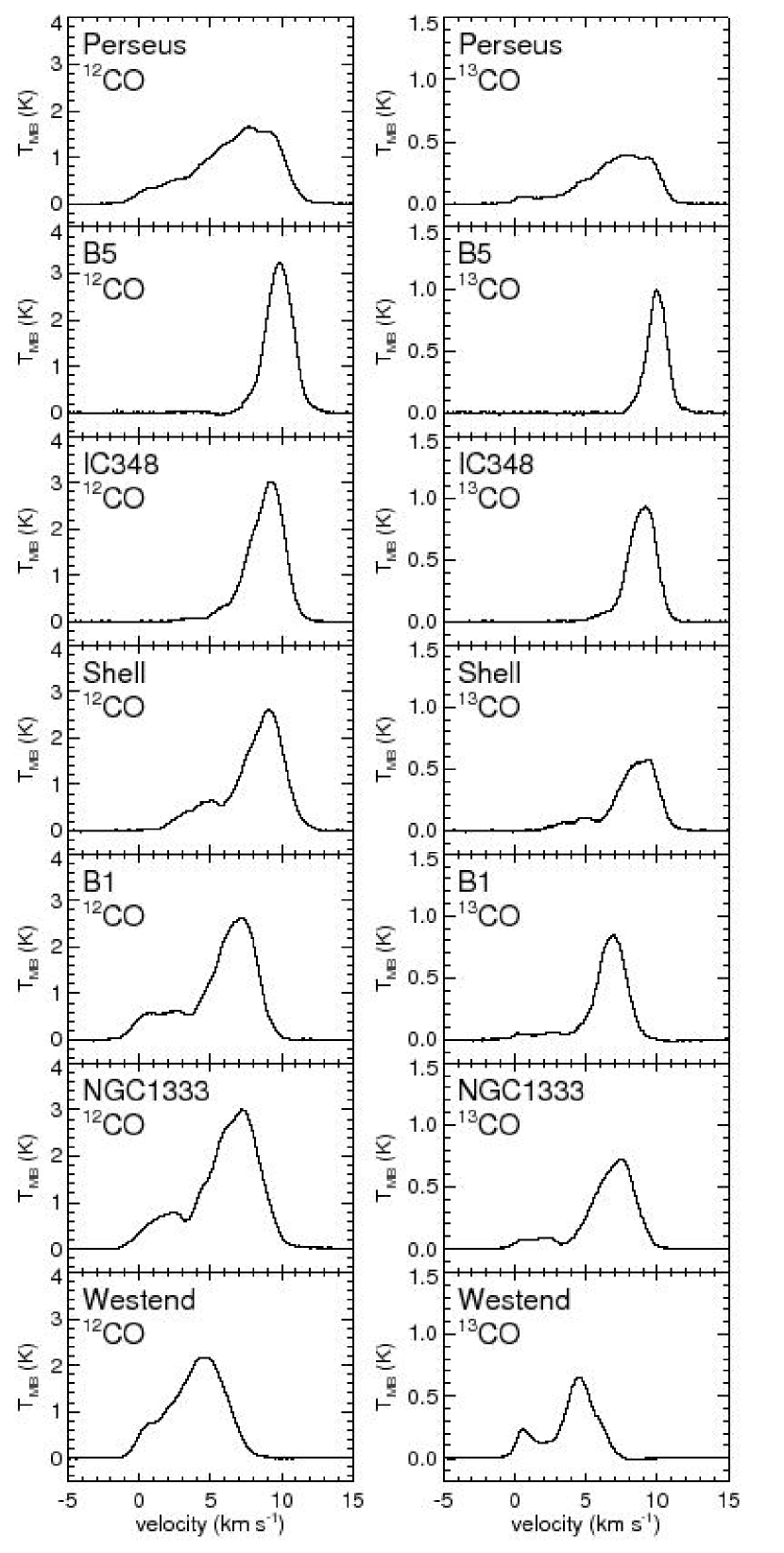
Figure 4: Average ¹²CO (1-0) and ¹³CO (1-0) spectra for all Perseus and the six sub-regions.

In Figure 4 we present the average ¹²CO and ¹³CO spectra for the whole cloud and each region, while in Table 2 we show the main properties derived from the average spectra. The central velocity and velocity dispersion are computed from the average ¹³CO with a Gaussian fit. We can see how different the region averages are from each other and the whole cloud. The gradient in central velocity across the cloud and the multiple components of the emission are clearly seen.

5 Analysis

5.1 Column Density Determination

To derive the H₂  column density, $N({\rm H_{2}})$, we assume that: (i) all the hydrogen traced by the derived extinction is in molecular form; (ii) the ratio between $N({\rm H})$ and $E(B-V)$ is $5.8\times 10^{21}~{}\rm{cm^{-2}\,mag^{-1}}$ as determined by Bohlin et al. (1978); and (iii) $R_{V}=3.1$, to obtain

$$\frac{N({\rm H_{2}})}{A_{V}}=9.4\times 10^{20}~{}\rm{cm^{-2}\ mag^{-1}}~{}.$$ (2)

The ratio measured by Bohlin et al. (1978) was calculated only for low extinctions, and it is not clear whether extrapolating to higher extinction regions is wise. In addition, it is well known that $R_{V}$ can increase up to values close to 4-6 in dense molecular clouds (see e.g. Draine, 2003), but we assume $R_{V}=3.1$ because it is the average value derived for the Milky Way and therefore our best estimation when this quantity has not been measured in the Perseus Cloud. This value of $R_{V}$ has also been used in all previous works, and therefore it facilitates the comparison.

To estimate ¹³CO column densities we assume that the emission is optically thin and in Local Thermodynamic Equilibrium (LTE). To estimate the LTE column density, we have to assume an excitation temperature, $T_{ex}$, and optical depth, $\tau$.

In general, the intensity of an emission line, $I_{line}$, is

$$I_{line}=(S-I_{0})(1-e^{-\tau}),$$ (3)

where $S$ is the source function and $I_{0}$ is the initial impinging radiation field intensity. The radiation temperature is defined as

$$T_{R}=I_{\nu}\frac{c^{2}}{2\nu^{2}k}~{},$$ (4)

where $I_{\nu}$ is the specific intensity and the filling factor is assumed to be unity. Assuming that the source function and initial intensity are black-bodies (with $I_{\nu}=B_{\nu}$) at $T_{ex}$ and $T_{bg}=2.7$ K, respectively, then we can write

$$T_{R} = T_{0}\left(\frac{1}{e^{T_{0}/T_{ex}}-1}-\frac{1}{e^{T_{0}/T_{bg}}-1}\right)(1-e^{-\tau})~{},$$ (5)

where $T_{0}=h\nu/k$.

Assuming that the ¹²CO (1-0) transition is optically thick, $\tau\rightarrow\infty$, and that $T_{max}({\rm{}^{12}CO})$ is the main beam brightness temperature at the peak of ¹²CO, we can derive the excitation temperature using eq. (5)

$$T_{ex} = \frac{5.5~{}{\rm K}}{\ln\left(1+5.5~{}{\rm K}/(T_{max}({\rm{}^{12}CO})+0.82~{}{\rm K})\right)},$$ (6)

where 5.5 K$\equiv h\nu({\rm{}^{12}CO})/k_{\rm B}$, with $\nu({\rm{}^{12}CO})$=115.3 GHz, the frequency of the ¹²CO (1-0) line.

Assuming that the excitation temperature of the ¹³CO (1-0) line is the same as for the ¹²CO (1-0) line, the optical depth of ¹³CO (1-0) can be derived from eq. (5),

$$\tau({\rm{}^{13}CO}) = -\ln\left(1-\frac{T_{max}({\rm{}^{13}CO})/5.3~{}{\rm K}}{1/(e^{5.3~{}{\rm K}/T_{ex}}-1)-0.16}\right)~{},$$ (7)

where $T_{max}({\rm{}^{13}CO})$ is the main beam brightness temperature at the peak of ¹³CO.

The formal error for the excitation temperature, $\sigma(T_{ex})$, is

$$\sigma(T_{ex})=\frac{\left[T_{ex}/\left(T_{max}({\rm{}^{12}CO})+0.82\right)\right]^{2}}{1+5.5/\left(T_{max}({\rm{}^{12}CO})+0.82\right)}\,\sigma_{12}~{},$$ (8)

where $\sigma_{12}$ is the error in the ¹²CO peak temperature determination. We estimate that $\sigma_{12}$ is $0.15\,T_{max}({\rm{}^{12}CO})$ to account for the calibration uncertainty.

Using the definition of column density (Rohlfs & Wilson, 1996) and expressions (6) and (7), we derive the ¹³CO column density as

$$N({\rm{}^{13}CO})=\left(\frac{\tau({\rm{}^{13}CO})}{1-e^{-\tau({\rm{}^{13}CO})}}\right)3.0\times 10^{14}\,\frac{W({\rm{}^{13}CO})}{1-e^{-5.3/T_{ex}}}~{}\rm{cm^{-2}}~{},$$ (9)

where the $W({\rm{}^{13}CO})$ is the integrated intensity along the line of sight in units of ${\rm K\,km\,s^{-1}}$. This approximation is accurate to within $15\%$ for $\tau({\rm{}^{13}CO})<2$ (Spitzer, 1968), and always overestimates the column density for $\tau({\rm{}^{13}CO})>1$ (Spitzer, 1968).

In the determination of the ¹³CO column density, we use the derived excitation temperature instead of the dust temperature because the dust and gas are only coupled at volume densities above $\simeq 10^{5}~{}{\rm cm^{-3}}$ (e.g. Goldsmith, 2001), which are typically not traced by ¹²CO and ¹³CO (1-0) data. Moreover, if the volume density of the gas falls below a few times $10^{3}~{}{\rm cm^{-3}}$ (the critical density of the 1-0 transition), the ¹²CO lines are expected to be subthermally excited.

5.2 Curve of Growth

Assuming LTE, the photon escape probability for a slab as a function of optical depth, $\beta(\tau)$, can be written as (Tielens, 2005)

$$\beta(\tau)=\left\{\begin{array}[]{ll}(1-\exp(-2.34\,\tau))/4.68\,\tau&\tau<7\\ 1/4\tau\left[\ln\left(\frac{\tau}{\sqrt{\pi}}\right)\right]^{1/2}&\tau>7\end{array}~{},\right.$$ (10)

and the Doppler broadening parameter, $b$, is related to the atomic weight, $A$, and the gas temperature, $T$, by

$$b=\sqrt{\frac{2\,k\,T}{m}}=0.1290\sqrt{\frac{T}{A}}~{}\rm{km\,s^{-1}}~{},$$ (11)

where $m$ is the mass of the observed molecule.

The curve of growth relates the optical depth and the Doppler broadening parameter, $b$, with the integrated intensity, $W$, by

$$W=\int T_{MB}\,dv=T_{R}\,b\,f(\tau)~{},$$ (12)

where

$$f(\tau)=2\int_{0}^{\tau}\beta(\tilde{\tau})\,d\tilde{\tau}$$ (13)

in the Rayleigh-Jeans regime. In the above expressions $T_{MB}$ is the main beam brightness temperature (which is equal to $T_{R}$ for a filling factor of unity).

Assuming that ¹³CO emission is optically thin and that the ratio between ¹³CO and ¹²CO is constant in the region, we can write the optical depth as

$$\tau({\rm{}^{12}CO})=a\,W({\rm{}^{13}CO})~{},$$ (14)

where $a$ is the conversion between $W({\rm{}^{13}CO})$ and ¹²CO optical depth.

6 Results

6.1 Curve of Growth Analysis

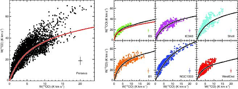
Figure 5: Integrated intensity of ¹²CO is plotted against the integrated intensity of ¹³CO. The left panel shows all data used while right panel shows each region separately, using the same colors as in Figure 3. The median of the 1-sigma errors are shown in bottom right of each plot. Solid lines are the growth curve fit, while the red curve in B5 is the fit from Langer et al. (1989).

As shown by Langer et al. (1989) in B5, ¹²CO  and ¹³CO integrated intensities are correlated and seem to be well described by the curve of growth (Spitzer, 1978). In Figure 5 we show ¹²CO and ¹³CO integrated intensities for Perseus and the individual regions defined in § 4. We perform a fit of the ¹²CO integrated intensity with a growth curve

$$W({\rm{}^{12}CO})=T_{R}\,b\int_{0}^{aW({\rm{}^{13}CO})}2\beta(\tilde{\tau})d\tilde{\tau}$$ (15)

and present the fit results in Table 3 and Figure 5.

The fits for the growth curve are very good, considering the simplicity of the model. However, it is clear that the correlation is better in the individual regions than in the complex as a whole, with the exception of Westend, in which the fit is less good. Our results for B5 nicely agree both in shape and amplitude with Langer et al. (1989) (red solid line in Figure 5).

From the fit results we see that for gas at $12~{}{\rm K}$ (intermediate value between average excitation temperature and dust temperature) the derived Doppler parameters for B5, IC348, B1 and Westend  are in reasonable agreement with $\sigma_{V}$ values listed in Table 2. In NGC1333 and the Shell, a larger Doppler parameter is expected because the emission comes from multiple components, as seen in Figure 4.

6.2 The X–factor: using ${\rm{}^{12}CO}$ to derive $A_{V}$

The integrated intensity along the line of sight of the ¹²CO (1-0) transition, $W({\rm{}^{12}CO})$, is often used to trace the molecular material. The conversion factor $X$,

$$N({\rm H_{2}})=X\,W({\rm{}^{12}CO}),$$ (16)

is derived, and to compare with previous results (e.g. Dame et al., 2001) it is calculated as

$$X=\left\langle\frac{9.4\times 10^{20}\,A_{V}}{W({\rm{}^{12}CO})}\right\rangle~{}.$$ (17)

However, the ¹²CO emission saturates at $A_{V}\sim 4$ mag in every region, as shown in Figure 6. Therefore, we perform the estimation of the $X$ factor in two ways: (i) for all the points, and (ii) for only those points with $A_{V}<4$ mag, where the column density can still be traced.

Figure 6 also shows that there is a threshold value of extinction below which no ¹²CO emission is detected. To take this into account we fit the linear function

$$A_{V}=A_{V12}+X_{2}\frac{W({\rm{}^{12}CO})}{9.4\times 10^{20}},$$ (18)

where $A_{V12}$ is the minimum extinction below which there is no ¹²CO emission and $X_{2}$ is the slope of the conversion (comparable to the $X$ factor). The linear fit is performed using the bivariate correlated errors and intrinsic scatter estimator (BCES), which takes into account errors in both axes and provides the least biased estimation of the slopes (Akritas & Bershady, 1996). The results of the $X$ factor and the linear fits are presented in Table CO isotopologues in the Perseus Molecular Cloud Complex: the $X$-factor and regional variations. In Figure 6, we show only the results for points with $A_{V}<4$ mag: a dotted line for the standard $X$ factor and a dashed line for the linear fit.

The values derived for $X$ using all the points (as previously done in the galactic determinations of $X$) are in agreement with the mean value of $(1.8\pm 0.3)\times 10^{20}~{}{\rm cm^{-2}\,K^{-1}\,km^{-1}\,s}$ derived by Dame et al. (2001) for the Milky Way. However, this fit is not good in the unsaturated regime ($A_{V}<4$ mag). Performing a linear fit to all of the data, including the saturated emission, can give unreasonable solutions, such as a negative minimum extinction needed to produce ¹²CO (1-0) integrated intensity.

The linear fit performed to positions with $A_{V}<4$ mag gives the best estimate for the extinction in the unsaturated regions but only provides a lower limit extinction estimate for the saturated regimes, while the standard $X$ factor provides a poor description of the data in both saturated and unsaturated regimes. The histograms of the errors associated with the conversions derived for positions with $A_{V}<4$ mag (bottom panels of Figure 6) show that the linear fit (open histogram) provides a more unbiased estimate of the extinction than the $X$ factor (filled histogram). This improvement in the precision of the extinction estimate goes along a reduction in the errors. The width of a Gaussian fitted to the histograms of the regions implies a typical error of 40% and 25% for the X factor and the linear fit, respectively. Performing the same analysis on the histograms of the whole cloud gives an error of 59% and 38% for the X factor and the linear fit, respectively.

However, as we can see from Figure 6 the linear relation is not very accurate for $A_{V}>4$ mag. Therefore, following the simplest solution of radiative transfer

$$I=I_{0}\left(1-e^{-\tau}\right)~{},$$

we fit it to our data with

$$W({\rm{}^{12}CO})=W_{0}\left(1-e^{-k(A_{V}-A_{k12})}\right)~{},$$ (19)

where $W_{0}$ is the integrated intensity at saturation, $A_{k12}$ is the minimum extinction needed to get ¹²CO emission, and $k$ is the conversion factor between the amount of extinction and the optical depth. We perform an unweighted fit of the non-linear function to the data, which yield solutions that better follow the overall shape of the $W({\rm{}^{12}CO})$ as a function of $A_{V}$. Unfortunately, the best fits for Westend and Perseus are quite poor and should be regarded with caution. The best parameters are listed in Table 5 and are shown in Figure 6 as solid curves. We note that the threshold extinction shows a large scatter, even in the more accurate non-linear fit. This suggests that different environmental conditions are causing the observed scatter (see § 7).

6.3 Using ${\rm{}^{13}CO}$ to derive ${\rm H_{2}}$ column densities

We expect the ¹³CO (1-0) transition to be optically thin at low extinction. If this is the case, a simple linear relation between the integrated intensity of ¹³CO and $A_{V}$ should fit the data,

$$A_{V}=W({\rm{}^{13}CO})\,B_{13}+A_{W13}~{}.$$ (20)

The fit is done using the BCES algorithm for points with $A_{V}$ $<5$ mag because there is some saturation in the emission. The results are presented in Table CO isotopologues in the Perseus Molecular Cloud Complex: the $X$-factor and regional variations and in Figure 7. Once again, we find that the minimum extinction needed to detect ¹³CO and the slope of the linear relation changes between the regions, though the variation is smaller than with the ¹²CO data. From Figure 7 we can clearly see the effect of saturation around 5 mag of extinction in IC348 and B1, similar to what was reported by Lada et al. (1994) in the more distant IC 5146, with comparable linear resolution. When comparing our results with the linear fit derived by Lada et al. (1994) we see that the fit parameters are quite different, suggesting that the IC 5146 cloud is quite different from Perseus. The linear fit for IC 5146 would indicate that for a region without extinction there is molecular emission, suggesting that the linear fit has been affected by points with saturated emission or that the fit errors are largely underestimated. Comparing our result for B5 with Langer et al. (1989), we find that the slopes are slightly different, but this can be reconciled by performing the linear fit taking all the points ($B_{13}=0.37\pm 0.1$, $A_{W13}=1.45\pm 0.04$) as done by Langer et al. (1989). However, the fit performed by Langer et al. (1989) was done using the extinction map derived by Bachiller & Cernicharo (1986), that is limited by $A_{V}$ values below 5 mag of visual extinction (due to a lack of detectable background stars). Also, given that their molecular data has a better resolution (1.5′) than the extinction map (2.5′), they interpolated the ¹³CO to the extinction positions instead of smoothing the data to the same resolution. Finally, the threshold extinction value differs from previous measurements mainly because it is hard to accurately define the zero point for extinction maps derived from optical star counting (as already mentioned, Schnee et al. 2005 reported a difference of $\sim 0.8$ mag).

Following the column density determination shown in § 5.1, which takes into account the effect of optical depth and excitation temperature, we investigate the relation between $N({\rm{}^{13}CO})$ and $A_{V}$, fitting a linear function to the data,

$$A_{V}=N({\rm{}^{13}CO})\,c+A_{V13},$$ (21)

where c and $A_{V13}$ are the parameters of the fit. From the fit we can derive the ratio of abundances between H₂ and ¹³CO as

$$\left[\frac{{\rm H_{2}}}{{\rm{}^{13}CO}}\right]=9.4\times 10^{20}\ c~{}.$$ (22)

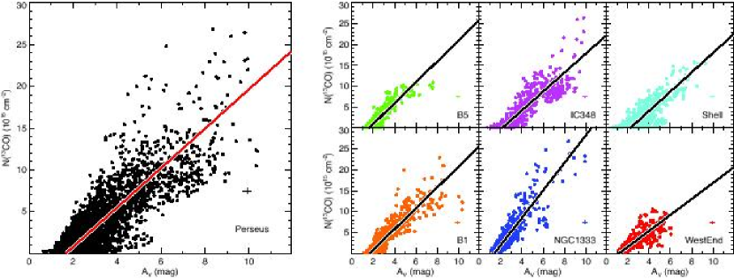
Figure 8: The left panel shows ¹³CO column densities as a function of visual extinction. The median of the 1-sigma errors are shown in bottom right of each plot. The excitation temperature is estimated using the ¹²CO  peak temperature, assuming this transition to be optically thick. The best fit is shown with a solid line. The right panel show the same as the left panel, but separated into different regions.

The result for the fit over the whole cloud and by regions is shown in Figure 8, and in Table CO isotopologues in the Perseus Molecular Cloud Complex: the $X$-factor and regional variations we present the best fit parameters. When performing the fit we estimate the error associated with the ¹³CO column density as 15%, due to the uncertainty in the calibration.

As shown in Figure 8, this relation presents a larger scatter, which is also present in individual regions (and it is consistent with previous work; see e.g. Combes, 1991). As already pointed out, selective photodissociation and/or chemical fractionation can alter the simple linear relation at low $A_{V}$ values, whereas optical depth may start to be large at high $A_{V}$ (see e.g. the tendency of $N({\rm{}^{13}CO})$ to flatten out at $A_{V}>5$ mag in B5, IC348 and B1).

The ¹³CO abundances derived from the fit present significant variations from region to region (see Table CO isotopologues in the Perseus Molecular Cloud Complex: the $X$-factor and regional variations). We do not find a correlation between the abundance and the threshold $A_{V13}$. This suggests that ${\rm{}^{13}CO}$ abundance variations are mainly due to different chemical/physical properties in the inner regions of the cloud at $A_{V}>A_{V13}$.

Comparing our results with those in Table CO isotopologues in the Perseus Molecular Cloud Complex: the $X$-factor and regional variations, we see that the abundances agree very well, within the errors, with previous values reported in Perseus, taking also into account the $\sim 0.8$ mag difference found by Schnee et al. (2005). This difference is produced by the difficulty in defining the zero level of extinction, which is harder in the optical star counting method than using NICER. The extinction threshold derived for Perseus is close to the one derived for $\rho$-Oph by Frerking et al. (1982), but they do not have any data at $A_{V}$ below $2.5$ mag and their determination has been done only for points with $A_{V}>4$ mag.

It is important to note that the numbers cited from previous works do not include the 10-20% calibration uncertainty that we do include in our results, and therefore our results are more accurate than previous ones.

6.4 Using ${\rm C^{18}O}$ to derive ${\rm H_{2}}$ column densities

We fit a linear relation between the integrated intensity of C¹⁸O and $A_{V}$,

$$A_{V}=W({\rm C^{18}O})\,B_{18}+A_{W18}~{}.$$ (23)

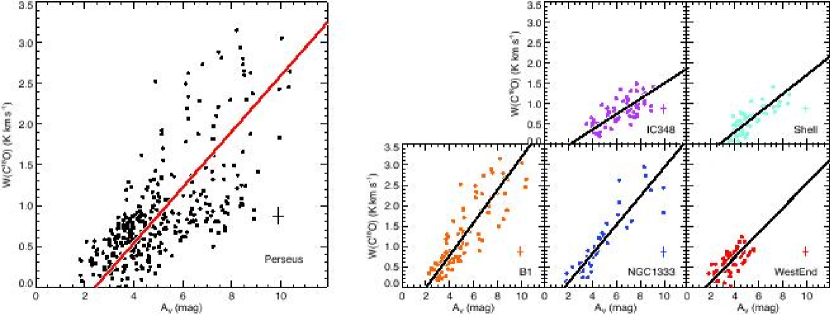
Figure 9: The left panel shows C¹⁸O integrated intensities as a function of visual extinction. The median of 1-sigma errors are shown in the bottom right corner of each plot. The best linear fit is shown with a solid line. The right panel shows the same as the left panel, but separated into different regions.

The fit results are presented in Table CO isotopologues in the Perseus Molecular Cloud Complex: the $X$-factor and regional variations and in Figure 9. We find that, as in the case of ¹²CO and ¹³CO, both parameters (extinction threshold and slope) vary between regions. However, due to the fewer points available per region, the errors are larger than for previous fits.

Despite the small number statistics, we still can see that C¹⁸O is fairly linear up to at least 10 mag. When comparing our results with the linear fit derived by Lada et al. (1994), we see that the fit parameters are quite different. However, they performed the fit over a wider $A_{V}$ range (up to 15 mag), and it is possible that despite their efforts the fit could have been affected by emission with higher optical depth.

Langer et al. (1989) derived a fit in B5. Unfortunately, we don’t have coverage for B5, and therefore no direct comparison can be done. Nevertheless, we find that the threshold extinction value derived for B5 is systematically lower than the values derived here for other regions (similar to what is found in ¹³CO) while the slope is in agreement (within the error bars) with the parameters derived here.

6.5 ${\rm{}^{12}CO}~{}(1-0)$ Excitation Temperature vs. Extinction

Being collisionally excited, the excitation temperature of ¹²CO (1-0) is expected to increase as we move from the outskirts of the cloud, where the extinction and volume densities may be lower than the critical density for the ¹²CO (1-0) transition, to the most extinguished and densest regions, where ¹²CO (1-0) is in LTE and faithfully traces the gas kinetic temperature.

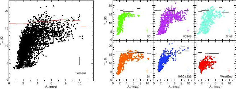
Figure 10: Excitation temperature derived using ¹²CO plotted against the visual extinction at the same position. The median of the 1-sigma errors are shown in bottom right of each plot. The solid line is the median dust temperature for each sample within the extinction bin. The left panel shows all data used while the right panel shows them separated by regions.

The excitation temperature, derived using ¹²CO  and eq. 6, is shown as a function of the visual extinction in Figure 10. In addition we plot the median dust temperature computed in bins of extinction as horizontal lines. When all the points are plotted (left panel of Figure 10) there is a poor correlation between excitation temperature and extinction. This is a direct result of mixing very different environments within the cloud in one plot. In fact, from the right panel of Figure 10, where the excitation temperature and visual extinction are plotted for individual regions, it is clear that the scatter is significantly lower and the excitation temperature rises from $\sim 5$ K at low $A_{V}$ ($\sim 2$ mag) up to a temperature close to the derived dust temperature in positions with $A_{V}>4$. The more quiescent regions (B1 and B5) present a smaller dispersion, whereas more active regions (IC348 and NGC1333) present a larger spread in the excitation temperature, probably because of the larger variation of physical conditions along the line of sight and/or the multiple velocity components. The region labeled as “Westend” has a very low excitation temperature when compared with the rest of the cloud. As shown in the right panel, in individual regions the dust temperature does not change more than approximately one degree except in the “Shell” which shows a steady increase with $A_{V}$, and in NGC1333 where a peak of the dust temperature is present at $A_{V}\sim 8$ mag, probably due to the internal heating produced by the nearby embedded cluster. On the other hand, the ¹²CO excitation temperature ranges between 5 and 20 K.

It is important to note that almost all the points lie below the median dust temperature of the region, indicating that ¹²CO is tracing gas at volume densities well below $10^{5}~{}{\rm cm^{-3}}$, the lower limit to have dust and gas coupling (Goldsmith, 2001). The average excitation temperature for points above 4 mag is $13.8$ K, while the standard deviation is $2.3$ K. We count the number of positions where the ¹²CO emission is sub-thermal ($T_{ex}<11.5$ K) obtaining that it is $\sim 60$ %. Westend is a region with ¹²CO excitation temperature always below the dust temperature. This could be due to a lower fraction of high density material compared to the other regions. It is interesting that in the regions in the North-East part of the cloud (B5, IC348 and Shell) the dust temperature is closer to 17 K while in the South-West part (B1, NGC1333 and Westend) it is closer to 16 K, suggesting variations in the ISRF across the Perseus Complex.

7 Modeling using PDR code

To relate the observed variations in the ¹²CO and ¹³CO lines with changes in the physical properties of the regions, we use the Meudon PDR code (Le Petit et al., 2006). This code includes most physical effects by explicit calculation; in particular it calculates the ¹²CO shielding, unlike the majority of other codes available (e.g. Röllig et al., 2007), where fitting formulae are used instead.

We use the abundances derived by Lee et al. (1998) (see table 9) for clouds with high metal abundances (more appropriate for the material traced by ¹²CO and ¹³CO) a ¹²C/¹³C abundance ratio of 80 and a cosmic-ray ionization rate of $\zeta=10^{-17}~{}\rm{s^{-1}}$ (a $\zeta$ value 6 times larger than the adopted one has also been considered, but found not to change the results by more than 10%; see Appendix). To reproduce the observed [H₂/¹³CO] ratio we increased the ¹²C abundance by a factor of 1.8 compared to Lee et al. (1998). To create curves of integrated intensity as a function of $A_{V}$, we run PDR models with different extinctions ($A_{V}$$=0.5,1,1.5,2,2.5,3,4,5,8,10$ mag). Each PDR calculation is performed over a grid of parameters, assuming a slab of constant density illuminated on both sides: (1) The turbulent velocity is fixed to the Doppler parameter derived from the curve of growth fit assuming $T_{R}=12$ K for each region (see Table 3 and § 6.1). (2) The volume density $n=10^{3},5\times 10^{3},10^{4},5\times 10^{4}~{}{\rm cm^{-3}}$. (3) The radiation field is $\chi=1\textrm{ and }3$ times the standard Draine’s radiation field (Draine, 1978) (other $\chi$ values have been explored and reported in the Appendix).

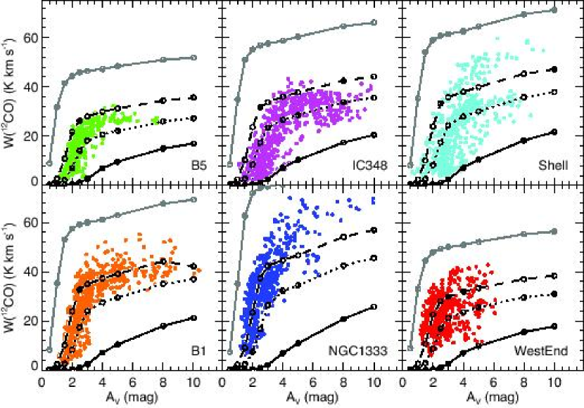
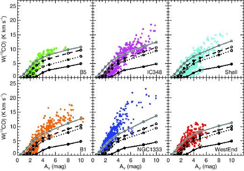
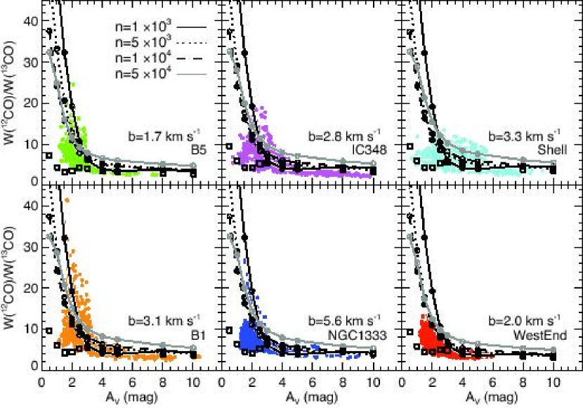
Figure 11: Results of the PDR modeling. Upper, middle and bottom panels show the comparison between $W({\rm{}^{12}CO})$, $W({\rm{}^{13}CO})$ and the ratio $W({\rm{}^{12}CO})/W({\rm{}^{13}CO})$ with $A_{V}$, respectively. Black and grey lines are derived from PDR models. Unconnected black squares show the ratio between ¹²CO and ¹³CO emission predicted by the PDR model with densities of $5\times 10^{3}$ and $1\times 10^{4}~{}{\rm cm^{-3}}$, respectively.

The observed values of $W({\rm{}^{12}CO})$, $W({\rm{}^{13}CO})$ and $W({\rm{}^{12}CO})/W({\rm{}^{13}CO})$ as a function of $A_{V}$ are compared with the models results in Figure 11. To perform this comparison, the PDR code output, $I=\int I_{\nu}d\nu$, is converted using the definition of brightness temperature (eq. 4):

$$W=\int T_{R}\,dv=\frac{I\,c^{2}}{2\nu_{0}^{2}k}\frac{c}{\nu_{0}}=\frac{c^{3}}{2\nu_{0}^{3}k}I~{},$$ (24)

and the ratio can be expressed as

$$\frac{W({\rm{}^{12}CO})}{W({\rm{}^{13}CO})}=\left(\frac{\nu({\rm{}^{13}CO})}{\nu({\rm{}^{12}CO})}\right)^{3}\frac{I({\rm{}^{12}CO})}{I({\rm{}^{13}CO})}$$ (25)

First, we note that PDR models are reasonably good in reproducing ¹²CO and ¹³CO observations, if one allows for variations in densities along different lines of sight. One exception is NGC1333, where the points with “excess” in ¹³CO emission are associated with positions just South of the NGC1333 stellar cluster, where a second velocity component is observed. This produces less saturation in the ¹³CO emission. Secondly, in the case of ¹³CO, the Doppler parameter (shown in the bottom panels of Figure 11) does not affect the results of PDR models within 10%, whereas for ¹²CO, differences of $\leq$40% are present above 2 mag of visual extinction. In fact, the ¹²CO line is optically thick, thus an increase in the line-width produces a significant increase in the line brightness because of the optical depth reduction. The insensitivity of ¹³CO integrated intensity to variations of the turbulent line-width leaves the density and radiation field as the two possible causes of the observed differences between the regions.

In Figure 11 we show only the effects of density with $\chi=1$. Small variations (within a factor of 3) of the radiation field intensity slightly shift the curves to higher or lower $A_{V}$ by 1 mag, if the radiation field is larger or smaller, respectively. The main conclusions for individual regions are listed below:

• B5: this is the most quiescent region in the whole Perseus complex. The best fit for the $W({\rm{}^{12}CO})$ is a PDR model of a cloud with a narrow range of density change, between $5\times 10^{3}$ and $1\times 10^{4}~{}{\rm cm^{-3}}$, values consistent with previous analysis. A similar density range is found to reproduce $W({\rm{}^{13}CO})$ at $A_{V}<4$ mag, whereas $5\times 10^{4}~{}{\rm cm^{-3}}$ is more appropriate for the emission at larger extinctions (higher density regions are mainly responsible for the ¹³CO emission at $A_{V}>4$ mag). We note that the integrated intensities of the two CO isotopologues approach (with increasing $A_{V}$) the lowest values in the whole sample, suggesting that denser material is hidden to view because of photon trapping in the narrow range of velocities observed in this region.

• IC348: in this cluster-forming region, the density spread is larger than in B5, with values ranging between $\rm{few}\times 10^{3}$ and $\simeq 1\times 10^{4}~{}{\rm cm^{-3}}$. Similarly, the ¹³CO at low $A_{V}$($<4$ mag) are reproduced by models with $10^{3}-10^{4}~{}{\rm cm^{-3}}$, whereas densities larger than $5\times 10^{4}~{}{\rm cm^{-3}}$ are needed above $4~{}$mag. However, the points at $A_{V}>7$ mag and $W({\rm{}^{13}CO})>12~{}{\rm K\,km\,s^{-1}}$ lie next to the embedded cluster, so that local heating and enhanced turbulence are probably increasing the ¹³CO brightness (the flattening of the $W({\rm{}^{13}CO})$ vs. $A_{V}$ curve is in fact less pronounced than in the case of B5, suggesting less optical depth). Thus, proto-stellar activity is locally affecting the ¹³CO emission, but not the ¹²CO.

• Shell: this region shows the largest spread in density for ¹²CO at all values of $A_{V}$ from $1\times 10^{3}$ to about $3\times 10^{4}~{}{\rm cm^{-3}}$. At $A_{V}>5$ mag the data groups around two separate values of $W({\rm{}^{12}CO})$: $\sim 35$ and $55~{}{\rm K\,km\,s^{-1}}$. The former group is associated with the (outer) shell reported in dust emission by Ridge et al. (2006b), whereas the latter is located in the inner part of the shell, maybe exposed to a larger radiation field causing more dissociation of CO molecules. The ¹³CO emission appears similar to IC348, with the exception of points located at low $W({\rm{}^{13}CO})$ (below $4~{}{\rm K\,km\,s^{-1}}$) and $A_{V}>4$ mag which are again associated with the inner part of the Shell. This also suggests some further destruction process for the ¹²CO.

• B1: the ¹²CO emission is consistent with material at densities between $5\times 10^{3}-3\times 10^{4}~{}{\rm cm^{-3}}$. Compared with B5, the B1 region shows brighter ¹²CO lines at lower (as well as higher) extinction. This is probably related to the larger Doppler parameter of B1. Several data points at low $A_{V}$ ($<$2 mag) are well reproduced by PDR models of dense clouds. The need of high densities at low $A_{V}$ also appears in the ¹³CO panel.

• NGC1333: this is the most active star forming site in the whole Perseus cloud and the behaviour of the ¹²CO and ¹³CO integrated intensities as a function of $A_{V}$ is in fact significantly different when compared to the other regions. First of all, the densities required in the PDR code to match the data are mostly above $10^{4}~{}{\rm cm^{-3}}$, both for the ¹²CO and ¹³CO emission. Secondly, the saturation of the ¹²CO line becomes evident only at $A_{V}>6$ mag (unlike $\sim 4$ mag, as in the other regions). Here, similarly to what is seen in B1, non-thermal motions driven by the embedded protostellar cluster are broadening the CO lines, allowing photons from deeper in the cloud to escape. The effect is more pronounced than in B1, consistent with the fact that NGC 1333 has the largest Doppler parameter among the six regions. We further note that, unlike in IC348, the ¹²CO (1-0) integrated intensity is also affected by the internal star formation activity, significantly reducing the saturation and enhancing the brightness at large $A_{V}$. Internal motions, likely driven by protostellar outflows, are thus more pronounced in NGC 1333 than in IC348, likely because of the larger star formation activity.

• Westend: this is the only region where no data points are present at $A_{V}>6$ mag, and the ¹²CO, as well as the ¹³CO, integrated intensity shows a large scatter between $A_{V}$ of 1 and 6 mag. These two facts are consistent with an overall lower density and probably clumpy medium, where relatively small high density clumps are located along some lines of sight, whereas a significant fraction of the data (19% of points in ¹²CO) can be reproduced by uniform PDR model clouds with densities below $5\times 10^{3}~{}{\rm cm^{-3}}$.

In general, model predictions for ¹³CO (1-0) can only reproduce well the observed emission at low extinction ($A_{V}<3$ mag). The complex structure of active star forming regions, in particular density and temperature gradients as well as clumpiness along the line of sight (all phenomena not included in the PDR code) can of course contribute to the deviations from the uniform PDR models. We point out again that the largest Doppler parameters, i.e. the largest amount of non–thermal (turbulent?) motions, are present in active regions of star formation, so their nature appears to be linked to the current star formation activity and not to be part of the initial conditions in the process of star formation.

In the bottom panel of Fig. 11, the $W({\rm{}^{12}CO})/W({\rm{}^{13}CO})$ ratio is shown as a function of $A_{V}$ for the six regions. The PDR models appear to reproduce well the integrated intensity ratio, for a broad range of $A_{V}$. As we just saw, the ¹³CO data preferentially trace higher density material than ¹²CO lines, so the black squares show the ratio between the ¹²CO and ¹³CO emission as predicted by PDR models with $5\times 10^{3}{\rm cm^{-3}}$ for ¹²CO and $1\times 10^{4}{\rm cm^{-3}}$ for ¹³CO lines. One thing to note in these plots is the large fraction of points at low $A_{V}$ and low $W({\rm{}^{12}CO})/W({\rm{}^{13}CO})$ which lie below the PDR model curves, in particular for B5, NGC 1333, and Westend, but they lie above the black squares showing that the PDR model with different densities can reproduce all the emission. Another way to reproduce these data points is by decreasing the interstellar radiation field by a factor of a few. Alternatively, it is possible that these lines of sight intercept material where the ¹³C carbon is still partially in ionized form, so that the reaction ${}^{13}\rm{C}^{+}+{\rm{}^{12}CO}\rightarrow\rm{{}^{12}C}^{+}+{\rm{}^{13}CO}+\Delta E$ (with $\Delta E/k=37$ K; Watson 1977) can proceed and enhance the ¹³CO abundance relative to ¹²CO.

We finally note here that Bell et al. (2006) have theoretically investigated the variation of the $X$ factor using UCL_PDR and Meudon PDR codes. They argue that variations in $X$ can be due to variations in physical parameters, such as the gas density, the radiation field and the turbulence, in agreement with our findings.

8 Summary and Conclusions

Using the FCRAO ¹²CO, ¹³CO and C¹⁸O data, and a NICER extinction map produced by COMPLETE we perform a calibration of the column density estimation using ¹²CO, ¹³CO and C¹⁸O emission in Perseus. We report the following results:

• We find a parameter space, $V_{LSR}({\rm{}^{12}CO})$–$T_{\rm d}$, in which different spatial regions of the Perseus Molecular Cloud Complex also cluster, and we designate six regions within the complex (see Figures 2 and 3). We note that the dust temperature decreases by about 1 K from North East to South West.

• The ¹²CO data can be modeled with a curve of growth. The fit parameters vary between the six regions and this causes much of the scatter in the $W({\rm{}^{12}CO})$ vs. $W({\rm{}^{13}CO})$ plot of the whole Perseus Complex. The parameters derived from the fits agree with a previous study of a sub-region of Perseus (B5) to within errors (see Figure 5).

• The $X$ factor, $X\equiv N({\rm H_{2}})/W({\rm{}^{12}CO})$, is derived from linear fits to the data both for the whole Perseus Complex and for the six regions. The ¹²CO saturates at different intensities in each region, depending on the velocity structure of the emission, the volume density and radiation field. When the linear fit is done only for the unsaturated emission, the $X$ factor is smaller than that derived for the Milky Way. However, larger values are obtained (closer to that found in the Milky Way) if all the points are included in the fit (see Figure 6 and Table CO isotopologues in the Perseus Molecular Cloud Complex: the $X$-factor and regional variations). The most active star forming region in Perseus (NGC 1333) has the lowest $X$ factor and the largest ¹³CO abundance among the six regions.

• The gas excitation temperature varies from 4 K to 20 K, it increases with $A_{V}$, and it is typically below the dust temperature at all $A_{V}$. This can be explained if a fraction ($\simeq$ 60%) of the ¹²CO (1-0) lines is sub-thermally excited, i.e. if the ¹²CO- emitting gas has volume densities below $\simeq 3\times 10^{3}~{}{\rm cm^{-3}}$.

• The column density of ¹³CO is derived taking into account the effect of optical depth and excitation temperature. We find that the threshold extinction above which ¹³CO (1-0) is detected is larger than has previously been reported. However, the fractional abundances (w.r.t. H₂ molecules) are in agreement with previous determinations. The difference with previous works is due to the superior zero-point calibration and larger dynamic range of the NICER extinction map, as compared to those derived from optical star counting (see Figure 8 and Table CO isotopologues in the Perseus Molecular Cloud Complex: the $X$-factor and regional variations).

• ¹³CO abundance variations between the regions do not correlate with the extinction threshold $A_{V13}$, suggesting that the main cause of the variation is likely due to the chemical/physical properties of shielded molecular material deeper into the cloud. The ¹²CO (1-0) and ¹³CO (1-0) lines saturates at $A_{V}>4,5$ mag, respectively, whereas C¹⁸O (1-0) line do not show signs of saturation up to the largest $A_{V}$ probed by our data (10 mag).

• Using the Meudon PDR code we find that the observed variations among the different regions can be explained with variations in physical parameters, in particular the volume density and internal motions. Large Doppler parameters imply large values of the CO integrated intensities (as expected for very optically thick lines) and are typically found in active star forming regions (the largest values of the Doppler parameter and $W({\rm{}^{12}CO})$ being associated with NGC 1333, the most active site of star formation in Perseus). On the other hand, quiescent regions such as B5 appears less bright in CO and only show a narrow range of CO integrated intensities as a function of $A_{V}$. This is likely due to the fact that the photons emitted from the higher density regions located deep into the cloud have similar velocities relative to the outer cloud envelope traced by ¹²CO, so that they are more easily absorbed. Thus, turbulent (or, more generally, non-thermal) motions appear to be a by-product of star formation, more than part of the initial conditions in the star formation process.

This work has shown that local variations in physical conditions significantly affect the relation between CO-isotopologue emission and $A_{V}$, contributing to the observed scatter. The use of a standard $X$ factor, $1.8\times 10^{20}\,{\rm cm^{-2}\,K^{-1}\,km^{-1}\,s}$, produces an overestimation of the cloud’s mass by $\sim 45\%$ when compared to the mass derived from the extinction map, while the lower limit for the mass derived using the linear fit to the unsaturated points underestimates the mass by a $\sim 15\%$. The $X$ factor (as well as the ¹³CO fractional abundance) depends on the star formation activity, with lower values associated with the more active (and turbulent) regions. Extinctions measured by using ¹³CO and previous conversions from the literature are typically underestimated by $\sim 0.8$ mag, so that more shielding is needed to produce the observed ¹³CO compared to previous findings.

Appendix A Effect of $\chi$ and $\zeta$ variation

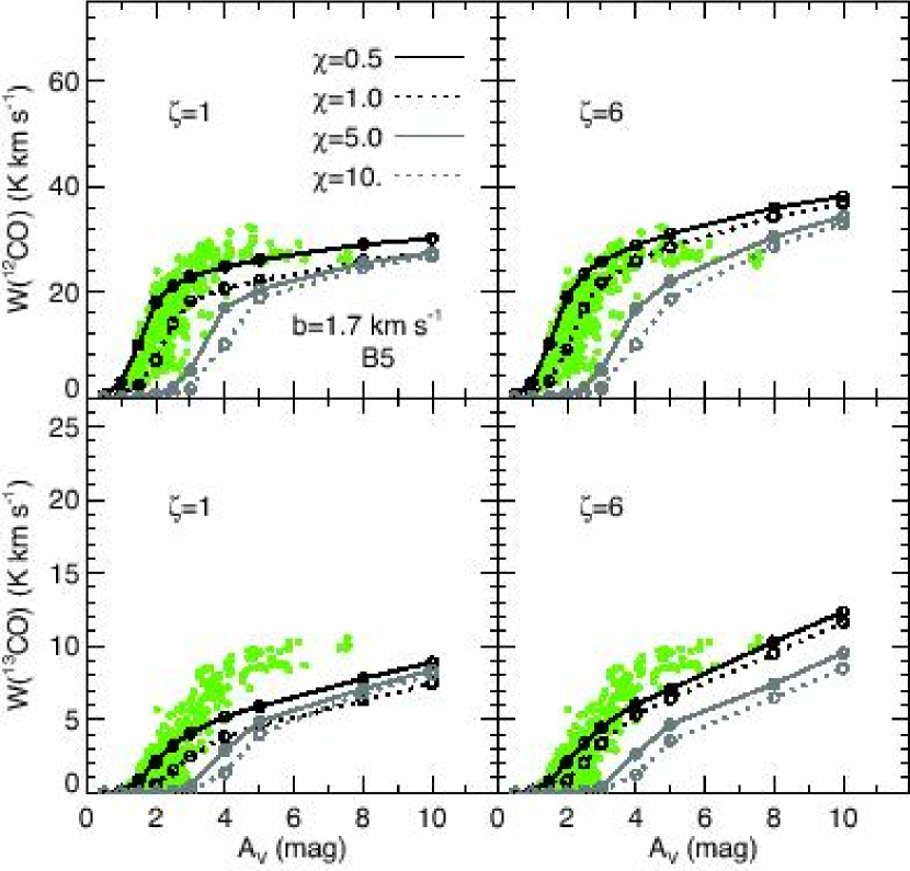
Figure 12: PDR results for the particular case of B5 and different values of $\chi$ and $\zeta$ (in units of $10^{-17}~{}\rm{s}^{-1}$). Black solid, black dotted, gray solid and gray dotted lines show the PDR model results for $\chi=0.5,1.0,5.0~{}{\rm and}~{}10$ times the standard Draine’s radiation field, respectively. Variations in $\chi$ mainly affect the low $A_{V}$ emission, whereas different $\zeta$ values slightly change the emission values at $A_{V}>4$ mag.

In Sect. 7 we have explored how changes in volume density and Doppler parameter affect the ¹²CO (1-0) and ¹³CO (1-0) integrated intensities ($W({\rm{}^{12}CO})$, $W({\rm{}^{13}CO})$) predicted by the Meudon PDR code. Here we show the effects of variations in the interstellar radiation field intensity, in units of Draine’s field ($\chi$), and the cosmic-ray ionization rate ($\zeta$) on $W({\rm{}^{12}CO})$ and $W({\rm{}^{13}CO})$. Fig. 12 shows the results of this parameter space exploration in the particular case of B5 and volume density of $5\times 10^{3}~{}{\rm cm^{-3}}$ (similar results apply to the other regions and different densities). The upper panels display the model results for $\chi$ values of 0.5, 1, 5 and 10: the main change is visible at $A_{V}<4$ mag, with a shift of the threshold extinction for ¹²CO and ¹³CO emission from about 1 to 3 mag for an increase of $\chi$ from 0.5 to 10, respectively.

The cosmic-ray ionization rate used in the PDR models described in Sect. 7 is $\zeta=1\times 10^{-17}$ s^-1. This value is quite uncertain and Dalgarno (2006) suggests a higher rate of $6\times 10^{-17}~{}\rm{s}^{-1}$ for molecular clouds (see also van der Tak & van Dishoeck, 2000). In the bottom panels of Fig. 12, we show the predicted $W({\rm{}^{12}CO})$ and $W({\rm{}^{13}CO})$ curves for $\zeta=6\times 10^{-17}~{}\rm{s}^{-1}$. The larger $\zeta$ value does not affect the CO emission at $A_{V}\leq 3$ mag, and only changes the integrated intensities by about 30%. Thus, the effect is not large enough to explain the largest $W({\rm{}^{13}CO})$ values.

Table 1: Clusters Regions Removed

Region	Center R.A.	Center Decl.	Box Size
	(deg)	(deg)	(deg2)
IC 348	56.088	32.171	0.480$\times$0.426
NGC 1333	52.212	31.483	0.397$\times$0.496

Table 2: Typical Properties of the Regions from Average Spectra

Region	$W({\rm{}^{12}CO})$	$T_{max}({\rm{}^{12}CO})$	$V_{LSR}({\rm{}^{12}CO})$	$\sigma_{V}({\rm{}^{12}CO})$	$W({\rm{}^{13}CO})$	$T_{max}({\rm{}^{13}CO})$	$V_{LSR}({\rm{}^{13}CO})$	$\sigma_{V}({\rm{}^{13}CO})$	$T_{ex}$	$\tau({\rm{}^{13}CO})$
	(K km s-1)	(K)	(km s-1)	(km s-1)	(K km s-1)	(K)	(km s-1)	(km s-1)	(K)
B5	8	3.2	9.84	0.90	1.6	0.99	9.99	0.64	12	0.31
IC348	9	3.0	9.01	1.18	2.2	0.93	8.99	0.95	12	0.35
Shell	10	2.6	8.73	1.49	2.0	0.58	8.72	1.30	11	0.28
B1	12	2.6	6.71	1.55	1.6	0.99	6.83	0.99	11	0.33
NGC1333	15	3.0	6.68	1.85	2.6	0.73	7.06	1.38	11	0.31
Westend	10	2.2	4.20	1.96	2.0	0.65	4.58	1.19	9	0.44
Perseus	11	1.7	7.26	2.65	2.2	0.39	7.67	2.15	11	0.34

Note. — $W\equiv$ integrated intensity. $T_{max}\equiv$ peak brightness temperature. $V_{LSR}\equiv$ centroid velocity. $\sigma_{V}\equiv$ velocity dispersion ($=\Delta v/\sqrt{8\ln{2}}$, where $\Delta v$ is the full width at half maximum). $T_{ex}\equiv$ excitation temperature derived from ¹²CO. $\tau\equiv$ ¹³CO optical depth. The 1-$\sigma$ uncertainty for integrated intensity, peak brightness and excitation temperature is estimated between 15 and 30%.

Table 3: Parameters for Growth Curve Fit

Region	$a$	$T_{R}\,b$
	(${\rm K^{-1}\,km^{-1}\,s}$)	(${\rm K\,km\,s^{-1}}$)
B5	0.61$\pm$0.03	20.5$\pm$0.5
IC348	0.246$\pm$0.007	33.5$\pm$0.6
Shell	0.223$\pm$0.009	40$\pm$1
B1	0.33$\pm$0.01	36.8$\pm$0.7
NGC1333	0.130$\pm$0.006	67$\pm$2
Westend	0.44$\pm$0.03	24.7$\pm$0.9
Perseus	0.260$\pm$0.004	35.9$\pm$0.4

Table 4: Linear fits to ¹²CO

Region	$X/10^{20}$	$A_{V12}$	$X_{2}/10^{20}$
	(${\rm cm^{-2}\,K^{-1}\,km^{-1}\,s}$)	(mag)	(${\rm cm^{-2}\,K^{-1}\,km^{-1}\,s}$)
Fit performed to the whole dataset
B5	2$\pm$1	0.0$\pm$0.2	1.5$\pm$0.1
IC348	3$\pm$2	0.51$\pm$0.08	1.61$\pm$0.07
Shell	2$\pm$1	1.0$\pm$0.1	1.09$\pm$0.08
B1	1.4$\pm$0.8	-0.6$\pm$0.1	1.38$\pm$0.09
NGC1333	0.9$\pm$0.3	-0.5$\pm$0.1	0.93$\pm$0.07
Westend	1.2$\pm$0.5	-1.8$\pm$0.3	1.8$\pm$0.4
Perseus	2$\pm$1	-0.33$\pm$0.07	1.38$\pm$0.05
Fit performed to points where $A_{V}<4$
B5	2$\pm$1	0.97$\pm$0.06	0.88$\pm$0.09
IC348	3$\pm$2	1.60$\pm$0.04	0.76$\pm$0.06
Shell	2$\pm$2	1.5$\pm$0.1	0.8$\pm$0.1
B1	1.4$\pm$0.9	1.18$\pm$0.04	0.56$\pm$0.04
NGC1333	0.9$\pm$0.3	0.60$\pm$0.06	0.57$\pm$0.06
Westend	1.1$\pm$0.4	-0.4$\pm$0.2	1.2$\pm$0.3
Perseus	2$\pm$1	0.92$\pm$0.04	0.72$\pm$0.04
Previous works
Galaxy (1)	2.8$\pm$0.4	$\cdots$	$\cdots$
$\rho$-Oph (2)	1.8$\pm$0.1	$\cdots$	$\cdots$
Galaxy (3)	1.8$\pm$0.3	$\cdots$	$\cdots$
Pipe (4)	$\cdots$	2.02$\pm$0.02	1.06$\pm$0.02

References. — (1) Bloemen et al. (1986); (3) Frerking et al. (1982); (3) Dame et al. (2001); (4) Lombardi et al. (2006);

Table 5: Parameters for ¹²CO Fit

Region	$W_{0}$	k	$A_{k12}$
	(${\rm K\,km\,s^{-1}}$)	(mag-1)	(mag)
B5	30.92	0.553	1.063
IC348	39.27	0.350	1.374
Shell	73.31	0.139	0.851
B1	43.08	0.691	1.309
NGC1333	67.12	0.374	0.748
Westend	30.45	0.529	-0.160
Perseus	42.29	0.367	0.580

Table 6: Results of Linear Fit to $W({\rm{}^{13}CO})$

Region	$A_{W13}$	$B_{13}$	Reference
	(mag)	(mag K-1 km-1 s)
B5	1.56$\pm$0.03	0.323$\pm$0.009	1
IC348	1.99$\pm$0.03	0.36$\pm$0.01	1
Shell	1.90$\pm$0.06	0.40$\pm$0.02	1
B1	1.64$\pm$0.03	0.296$\pm$0.009	1
NGC1333	1.19$\pm$0.03	0.26$\pm$0.01	1
Westend	0.75$\pm$0.06	0.44$\pm$0.02	1
Perseus	1.46$\pm$0.02	0.345$\pm$0.006	1
Previous works
IC 5146	-2.6$\pm$0.3	1.4$\pm$0.1	2
B5	0.54$\pm$0.13	0.39$\pm$0.02	3

References. — (1) This work, linear fit for $A_{V}<5$; (2) Lada et al. (1994), linear fit for $A_{V}<5$; (3) Langer et al. (1989)

Table 7: Results of Linear Fit to $N({\rm{}^{13}CO})$

Region	$A_{V13}$	c	[H2/13CO]	Reference
	(mag)	(mag cm-2)	$\times 10^{5}$
B5	1.62$\pm$0.04	(4.0$\pm$0.2)$\times 10^{-16}$	3.8$\pm$0.2	1,a
IC348	2.15$\pm$0.04	(4.4$\pm$0.1)$\times 10^{-16}$	4.1$\pm$0.1	1,a
Shell	2.23$\pm$0.05	(4.3$\pm$0.1)$\times 10^{-16}$	4.1$\pm$0.1	1,a
B1	1.68$\pm$0.04	(4.0$\pm$0.1)$\times 10^{-16}$	3.8$\pm$0.1	1,a
NGC1333	1.44$\pm$0.04	(3.0$\pm$0.1)$\times 10^{-16}$	2.8$\pm$0.1	1,a
Westend	1.19$\pm$0.05	(5.2$\pm$0.2)$\times 10^{-16}$	4.9$\pm$0.2	1,a
Perseus	1.67$\pm$0.02	(4.24$\pm$0.07)$\times 10^{-16}$	3.98$\pm$0.07	1,a
Previous works
Perseus B5	0.5$\pm$0.1	(3.8$\pm$0.2)$\times 10^{-16}$	3.6$\pm$0.2	2,b
Perseus	0.8$\pm$0.4	(4.0$\pm$0.8)$\times 10^{-16}$	3.8$\pm$0.8	3,b
L1495	0.3$\pm$0.3	(4.5$\pm$0.6)$\times 10^{-16}$	4.2$\pm$0.6	4,b
L1517	0.3$\pm$0.5	(6$\pm$2)$\times 10^{-16}$	5$\pm$1	4,b
$\rho$-Oph	1.6$\pm$0.3	(3.7$\pm$0.4)$\times 10^{-16}$	3.5$\pm$0.4	5,c
Taurus	1.0$\pm$0.2	(7.1$\pm$0.7)$\times 10^{-16}$	6.7$\pm$0.7	5,c

Note. — (a) $A_{V}$ derived from NIR colors, (b) $A_{V}$ derived from star counting; (c) $A_{V}$ derived using spectra.

References. — (1) This work; (2) Langer et al. (1989); (3) Bachiller & Cernicharo (1986); (4) Duvert et al. (1986); (5) Frerking et al. (1982)

Table 8: Results of Linear Fit to $W({\rm C^{18}O})$

Region	$A_{W18}$	$B_{18}$	Reference
	(mag)	(mag K-1 km-1 s)
IC348	2.1$\pm$0.4	5$\pm$11	1
Shell	2.7$\pm$0.3	4$\pm$7	1
B1	2.1$\pm$0.1	2.5$\pm$0.9	1
NGC1333	1.7$\pm$0.2	3$\pm$2	1
Westend	1.6$\pm$0.3	3$\pm$5	1
Perseus	2.4$\pm$0.1	2.9$\pm$0.9	1
Previous works
IC 5146	-0.7$\pm$0.3	10$\pm$1	2
B5	1.40$\pm$0.22	1.8$\pm$0.13	3

References. — (1) This work; (2) Lada et al. (1994), linear fit for $A_{V}<15$; (3) Langer et al. (1989)

Table 9: Initial chemical abundances with respect to total Hydrogen

Element	Abundance
He	$0.1$
C+	$1.307\times 10^{-4}$
13C+	$1.633\times 10^{-6}$
N	$2.14\times 10^{-5}$
O	$1.76\times 10^{-4}$
S+	$8.00\times 10^{-6}$
Fe+	$3.00\times 10^{-7}$

Figure 6: Top: Integrated intensity of ¹²CO and visual extinction derived using NICER. The left panel shows all data used and the right panel shows each region separately, using the same colors as in Figure 3. Solid lines show the best fit of eq. (19), dotted and dashed lines are the standard $W({\rm{}^{12}CO})\,X=N({\rm H_{2}})$ and straight line fits are only for points below $A_{V}$=4, respectively. Bottom: Histograms of the difference between the observed and expected $A_{V}$ for all data displayed in top panels. Filled and open histograms are for the standard $X$ factor and linear conversion, shown as dotted and dashed lines in upper panels, respectively.

Figure 7: Left panel shows ¹³CO  Integrated intensity compared with the extinction. The median of 1-sigma errors are shown in the bottom right corner of each plot. The best linear fit is shown with a solid line. The right panel shows same plots as the left panel, but for the individual regions.

References

- Akritas & Bershady (1996) Akritas, M. G., & Bershady, M. A. 1996, ApJ, 470, 706
- Alves et al. (2007) Alves, J., Lombardi, M., & Lada, C. J. 2007, In prep.
- Arce & Goodman (1999) Arce, H. G., & Goodman, A. A. 1999, ApJ, 517, 264
- Bachiller & Cernicharo (1986) Bachiller, R., & Cernicharo, J. 1986, A&A, 166, 283
- Bell et al. (2006) Bell, T. A., Roueff, E., Viti, S., & Williams, D. A. 2006, MNRAS, 371, 1865
- Bensch (2006) Bensch, F. 2006, A&A, 448, 1043
- Bloemen et al. (1986) Bloemen, J. B. G. M., Strong, A. W., Mayer-Hasselwander, H. A., Blitz, L., Cohen, R. S., Dame, T. M., Grabelsky, D. A., Thaddeus, P., Hermsen, W., & Lebrun, F. 1986, A&A, 154, 25
- Bohlin et al. (1978) Bohlin, R. C., Savage, B. D., & Drake, J. F. 1978, ApJ, 224, 132
- Cambrésy (1999) Cambrésy, L. 1999, A&A, 345, 965
- Cernicharo & Bachiller (1984) Cernicharo, J., & Bachiller, R. 1984, A&AS, 58, 327
- Combes (1991) Combes, F. 1991, ARA&A, 29, 195
- Dalgarno (2006) Dalgarno, A. 2006, Proceedings of the National Academy of Science, 103, 12269
- Dame et al. (2001) Dame, T. M., Hartmann, D., & Thaddeus, P. 2001, ApJ, 547, 792
- de Vries et al. (1987) de Vries, H. W., Thaddeus, P., & Heithausen, A. 1987, ApJ, 319, 723
- Draine (1978) Draine, B. T. 1978, ApJS, 36, 595
- Draine (2003) —. 2003, ARA&A, 41, 241
- Duvert et al. (1986) Duvert, G., Cernicharo, J., & Baudry, A. 1986, A&A, 164, 349
- Elias (1978) Elias, J. H. 1978, ApJ, 224, 453
- Frerking et al. (1982) Frerking, M. A., Langer, W. D., & Wilson, R. W. 1982, ApJ, 262, 590
- Goldsmith (2001) Goldsmith, P. F. 2001, ApJ, 557, 736
- Goodman et al. (2007) Goodman, A. A., Pineda, J. E., & Schnee, S. L. 2007, In prep.
- Hatchell & van der Tak (2003) Hatchell, J., & van der Tak, F. F. S. 2003, A&A, 409, 589
- Hily-Blant et al. (2005-1) Hily-Blant, P., Pety, J., & S., G. 2005-1, CLASS evolution: I. Improved OFT support, Tech. rep., IRAM
- Lada et al. (1994) Lada, C. J., Lada, E. A., Clemens, D. P., & Bally, J. 1994, ApJ, 429, 694
- Langer et al. (1989) Langer, W. D., Wilson, R. W., Goldsmith, P. F., & Beichman, C. A. 1989, ApJ, 337, 355
- Le Petit et al. (2006) Le Petit, F., Nehmé, C., Le Bourlot, J., & Roueff, E. 2006, ApJS, 164, 506
- Lee et al. (1998) Lee, H.-H., Roueff, E., Pineau des Forets, G., Shalabiea, O. M., Terzieva, R., & Herbst, E. 1998, A&A, 334, 1047
- Lombardi & Alves (2001) Lombardi, M., & Alves, J. 2001, A&A, 377, 1023
- Lombardi et al. (2006) Lombardi, M., Alves, J., & Lada, C. J. 2006, A&A, 454, 781
- Miville-Deschênes & Lagache (2005) Miville-Deschênes, M.-A., & Lagache, G. 2005, ApJS, 157, 302
- Padoan et al. (1999) Padoan, P., Bally, J., Billawala, Y., Juvela, M., & Nordlund, Å. 1999, ApJ, 525, 318
- Ridge et al. (2006a) Ridge, N. A., Di Francesco, J., Kirk, H., Li, D., Goodman, A. A., Alves, J. F., Arce, H. G., Borkin, M. A., Caselli, P., Foster, J. B., Heyer, M. H., Johnstone, D., Kosslyn, D. A., Lombardi, M., Pineda, J. E., Schnee, S. L., & Tafalla, M. 2006a, AJ, 131, 2921
- Ridge et al. (2006b) Ridge, N. A., Schnee, S. L., Goodman, A. A., & Foster, J. B. 2006b, ApJ, 643, 932
- Rieke & Lebofsky (1985) Rieke, G. H., & Lebofsky, M. J. 1985, ApJ, 288, 618
- Röllig et al. (2007) Röllig, M., et al. 2007, A&A, 467, 187
- Rohlfs & Wilson (1996) Rohlfs, K., & Wilson, T. L. 1996, Tools of Radio Astronomy (Tools of Radio Astronomy, XVI, 423 pp. 127 figs., 20 tabs.. Springer-Verlag Berlin Heidelberg New York. Also Astronomy and Astrophysics Library)
- Schnee et al. (2006) Schnee, S., Bethell, T., & Goodman, A. 2006, ApJ, 640, L47
- Schnee et al. (2008) Schnee, S. L., Li, J. G., Goodman, A. A., & Sargent, A. I. 2008, In prep.
- Schnee et al. (2005) Schnee, S. L., Ridge, N. A., Goodman, A. A., & Li, J. G. 2005, ApJ, 634, 442
- Solomon et al. (1987) Solomon, P. M., Rivolo, A. R., Barrett, J., & Yahil, A. 1987, ApJ, 319, 730
- Spitzer (1968) Spitzer, L. 1968, Diffuse matter in space (New York: Interscience Publication, 1968)
- Spitzer (1978) —. 1978, Physical processes in the interstellar medium (New York Wiley-Interscience, 1978. 333 p.)
- Strong & Mattox (1996) Strong, A. W., & Mattox, J. R. 1996, A&A, 308, L21
- Tielens (2005) Tielens, A. G. G. M. 2005, The Physics and Chemistry of the Interstellar Medium (The Physics and Chemistry of the Interstellar Medium, by A. G. G. M. Tielens, pp. . ISBN 0521826349. Cambridge, UK: Cambridge University Press, 2005.)
- van der Tak & van Dishoeck (2000) van der Tak, F. F. S., & van Dishoeck, E. F. 2000, A&A, 358, L79
- Watson (1977) Watson, W. D. 1977, in ASSL Vol. 67: CNO Isotopes in Astrophysics, ed. J. Audouze, 105–114
- Wilson et al. (1970) Wilson, R. W., Jefferts, K. B., & Penzias, A. A. 1970, ApJ, 161, L43+
- Young et al. (1982) Young, J. S., Goldsmith, P. F., Langer, W. D., Wilson, R. W., & Carlson, E. R. 1982, ApJ, 261, 513
- Young & Scoville (1982) Young, J. S., & Scoville, N. 1982, ApJ, 258, 467