High and Intermediate-Mass Young Stellar Objects in the Large Magellanic Cloud

Abstract

Archival Spitzer IRAC and MIPS observations of the Large Magellanic Cloud (LMC) have been used to search for young stellar objects (YSOs). We have carried out independent aperture photometry of these data and merged the results from different passbands to produce a photometric catalog. To verify our methodology we have also analyzed the data from the SAGE and SWIRE Legacy programs; our photometric measurements are in general agreement with the photometry released by these programs. A detailed completeness analysis for our photometric catalog of the LMC show that the 90% completeness limits are, on average, 16.0, 15.0, 14.3, 13.1, and 9.2 mag at 3.6, 4.5, 5.8, 8.0, and 24 $\mu$m, respectively.

Using our mid-infrared photometric catalogs and two simple selection criteria, [4.5]$-$[8.0]$>$2.0 to exclude normal and evolved stars and [8.0]$>$14$-$([4.5]$-$[8.0]) to exclude background galaxies, we have identified a sample of 2,910 sources in the LMC that could potentially be YSOs. We then used the Spitzer observations complemented by optical and near-infrared data to carefully assess the nature of each source. To do so we simultaneously considered multi-wavelength images and photometry to assess the source morphology, spectral energy distribution (SED) from the optical through the mid-infrared wavelengths, and the surrounding interstellar environment to determine the most likely nature of each source.

From this examination of the initial sample, we suggest 1,172 sources are most likely YSOs. We have also identified 1,075 probable background galaxies, consistent with the expected number estimated from the SWIRE survey. Spitzer IRS observations of 269 of the brightest YSOs from our sample have confirmed that $\gtrsim$95% are indeed YSOs. Examination of color-color and color-magnitude diagrams shows no simple criteria in color-magnitude space that can unambiguously separate the LMC YSOs from all AGB/post-AGB stars, planetary nebulae, and background galaxies.

A comprehensive search for YSOs in the LMC has also been carried out by the SAGE team and reported by Whitney et al. (2008). There are three major differences between these two searches. (1) In the common region of color-magnitude space, $\sim$850 of our 1,172 probable YSOs are missed in the SAGE YSO catalog because their conservative point source identification criteria have excluded YSOs superposed on complex stellar and interstellar environments. (2) About 20–30% of the YSOs identified by the SAGE team are sources we classify as background galaxies. (3) the SAGE YSO catalog identifies YSO in parts of color-magnitude space that we excluded and thus contains more evolved or fainter YSOs missed by our analysis. The shortcomings and strengths of both these YSO catalogs should be considered prior to statistical studies of star formation in the LMC. Finally, the mid-infrared luminosity functions in the IRAC bands of our most likely YSO candidates in the LMC can be well described by $N(L)\propto L^{-1}$, which is consistent with the Salpeter initial mass function if a mass-luminosity relation of $L\propto M^{2.4}$ is adopted.

1 Introduction

Star formation is one of the most fundamental processes that shape the observable universe. In particular, the formation of massive stars dramatically alters their local environment as their strong UV radiation field, stellar winds and eventual explosions as supernovae inject energy into the surrounding interstellar medium (ISM). This stellar energy feedback may compress the ambient medium to induce subsequent star formation, but may also disperse the natal molecular clouds to regulate further star formation. The onset and propagation of star formation plays an important role in the evolution of a galaxy.

Investigations of the star formation process using individually resolved young stars have been conducted for regions in our Milky Way galaxy. The formation of low-mass stars can be studied in great detail in nearby star forming regions (e.g., Taurus-Auriga Molecular Cloud; Kenyon & Hartmann, 1995; Hartmann et al., 2005), but the formation of stars more massive than a few solar masses cannot be studied easily because such stars are rarer and are often found in distant regions toward which the line-of-sight obscuration and confusion in the Galactic plane limits our ability to obtain a clear view. A global view of star formation in the Galaxy is particularly impossible.

The Spitzer Space Telescope, with its high angular resolution and sensitivity at mid- and far-infrared (IR) wavelengths, has provided not only a better view of the formation of individual massive and low-mass stars in the Galaxy, but also a new opportunity to study massive star formation in nearby galaxies, most notably the Large Magellanic Cloud (LMC). In the LMC, because of its close proximity (50 kpc, where 1″=0.25 pc; Feast, 1999) and low inclination ($\sim 30^{\circ}$; Nikolaev et al., 2004), massive and intermediate-mass young stellar objects (YSOs) can be resolved by Spitzer and inventoried throughout the entire galaxy.

In this paper we consider YSOs to be young stars still in the process of forming, as YSO candidates selected based on mid-IR Spitzer observations have already formed a compact source at the center. Furthermore, the linear resolution of Spitzer observations, $>$50,000 AU, means that a central source and its surrounding circumstellar material cannot be separated. Thus, the emission would include not only the central source but also any circumstellar disk, and/or circumstellar envelope. In terms of Class 0/I/II/III system used to describe low-mass YSOs (Lada, 1987), we expect to be biased toward high and intermediate-mass systems that are more similar to the Class I and II sources. In other words, sources that have formed a central source but which may still be in the process of actively accreting material. As such, the central objects are most likely young pre-main sequence stars.

This inventory of massive and intermediate-mass YSOs, combined with the well-surveyed ISM and stars, can be used to study the relationship between star formation and gravitational instability on a global scale (e.g., Yang et al., 2007), as well as triggered star formation on local scales (e.g., Chu et al., 2005; Caulet et al., 2008; Chen et al., 2009). It is also possible to investigate whether the mass function of the newly formed stars depends on the interstellar conditions that lead to the star formation (e.g., Chu & Gruendl, 2008).

In this paper we present the results of a search for YSOs in the LMC using Spitzer observations and complementary optical and near-IR observations. In §2 we describe the observations used for this search. In §3 we examine the mid-IR photometry, compare our results and methodology with those from two other wide-area surveys using Spitzer, and examine the completeness and reliability of our results. In §4 we describe the methodology to search for YSOs using the photometric results and in §5 we present the results of this search. Finally, in §6 we discuss the populations of sources that we identify, compare them with the results from a previous YSO survey, and discuss the implications of these results for studying the detailed star formation in the LMC.

2 Observations and Data Reduction

2.1 Data Set

The LMC has been observed by the Spitzer Space Telescope using the InfraRed Array Camera (IRAC; Fazio et al., 2004) and the Multiband Imaging Photometer for Spitzer (MIPS; Rieke et al., 2004). We have used the archival data from the Spitzer Legacy program Surveying the Agents of a Galaxy’s Evolution (SAGE; Meixner et al., 2006) that mapped the central 7${}^{\circ}\times$7^∘ area of the LMC, along with numerous earlier programs that targeted star-formation complexes throughout the LMC (see Table 1 for summary). We have downloaded both the BCD (Basic Calibrated Data) and post-BCD pipeline processed products for each of the programs listed as they became available. More information on the instruments and pipeline processing can be found at the Spitzer Science Center’s Observer Support website.

2.2 IRAC Data Reduction

For the IRAC observations we have used the post-BCD products to make photometric measurements of all sources in the IRAC 3.6, 4.5, 5.8, and 8.0 $\mu$m bands. The DAOFIND task in IRAF was used to search for sources in the IRAC post-BCD images with the sharpness and roundness criteria optimized to: account for the point-spread function (PSF) afforded by IRAC, aid in the rejection of cosmic-ray hits, and identify sources amid a complex background. We found the ranges for these two criteria to identify the largest numbers of reliable sources were: $0.6\geq sharpness\geq 1.0$ and $-0.7\geq roundness\geq 0.7$. The PHOT task was then used to obtain photometric extractions from a 3$\farcs$6 radius aperture centered on each source and a 3$\farcs$6–8$\farcs$4 annular background region. To determine source brightnesses we then applied the aperture corrections and flux calibrations tabulated in the IRAC Data Analysis Handbook ver2.0. When observations were obtained with the high dynamic range mode, photometric measurements were also extracted from the short-exposure images to obtain measurements for sources at or near saturation in the long exposures. In Table 2 we summarize the photometric parameters, aperture corrections, zero-points, and the assumed flux calibration accuracy used when analyzing the IRAC observations.

At each location in the LMC there are usually IRAC observations for at least two epochs. The photometric results in each band were compared and combined where individual measurements were weighted by the inverse square of their photometric uncertainty. The post-BCD images contain numerous transient sources, including cosmic-ray hits, ghost images of bright sources, and latent images of bright sources from prior frames. To remove the transient sources we first relied on the above-mentioned sharpness and roundness criteria to reject sources that are significantly more peaked or less circular than the IRAC PSF. Further rejection of transients was accomplished when combining data from different epochs by eliminating “sources” that should have had statistically significant counterparts at other epochs. An assessment of the resulting photometric reliability and completeness for the IRAC measurements are made in § 3.

In order to match sources between different IRAC bands we then cross-correlated the locations of sources between bands. This was accomplished by an algorithm which first intercompared each pair of IRAC bands singly and then reconciled those sets of comparison with one another. For the IRAC measurements, positions were considered to match if they were within 1$\farcs$5. This process often results in “orphan” sources that have a detection in only one band (most typically the 3.6 $\mu$m band). On rare occasions a “degenerate” match can occur, where a source in one band is matched to multiple sources in another band. For these cases the closest match was assumed to be correct. The resulting photometric catalog has $>$3.5 million IRAC sources where the position of each source is formed by the weighted mean of the positions found in the individual bands.

2.3 MIPS Data Reduction

Most of the MIPS observations in the LMC have used the scan map mode with either a medium or fast scan rate. For the MIPS 24 and 70 $\mu$m observations we used the MOPEX software to construct new mosaics from all available BCD data with 1$\farcs$245 and 4$\farcs$0 pixels ($\sim\frac{1}{2}$ the original resolution), respectively. Prior to building each mosaic we removed brightness offsets between the individual frames by solving for the best offset for each frame using the method outlined in Regan & Gruendl (1995). In this image reconstruction we relied on the fact that the SAGE MIPS observations usually had at least two scans at nearly orthogonal directions to remove most of the bright latent images that occurred after the MIPS detectors encounter bright emission. Some artifacts could remain in these images.

In the case of the MIPS 24 $\mu$m reconstructed images we again searched for sources using the DAOFIND task and then performed aperture photometry using the PHOT package in IRAF. The photometric extractions used a 6″ radius aperture centered on the source with a 15-23″ annular region to measure the background flux. These aperture sizes were chosen to allow us to analyze sources with as small a separation as possible while also minimizing background contamination by placing the sky aperture between the first and second Airy rings. We used isolated bright sources to independently determine the aperture correction and found a value of 1.798. Our value is high compared to the typical values of 1.69 tabulated in the MIPS Data Analysis Handbook (versions 3.2 and earlier), but recent work by Fadda et al. (2006) measuring the curve of growth for MIPS 24 $\mu$m observations results in aperture corrections of 1.78 and 1.84 for a theoretical PSF and an empirical determination from the Spitzer Extragalactic First Look Observations, respectively. We have used our aperture correction to determine source brightnesses at 24 $\mu$m throughout this work.

Similar to the IRAC observations, there exist MIPS 24 $\mu$m observations at two or more epochs for nearly all locations. Thus transients not rejected by MOPEX are mostly rejected when we combine all 24 $\mu$m photometric measurements using the same methods and criteria used for the IRAC measurements. The final catalog at 24 $\mu$m has 53,800 sources. These source locations have been cross-correlated with and incorporated into the merged IRAC catalog for 24 $\mu$m sources within 1$\farcs$5 of an IRAC source. Here multiple matches are not possible because the MIPS 24 $\mu$m PSF has a full-width at half maximum of $\sim$6″. An assessment of the resulting photometric reliability and completeness for the MIPS 24 $\mu$m measurements are made in § 3.

In the case of the MIPS 70 $\mu$m observations, rather than a blind search for sources using the DAOFIND task, we have made photometric measurements for two situations. First, we measure fluxes for 70 $\mu$m sources where we have identified an unambiguous counterpart in the 70 $\mu$m images for sources previously identified with IRAC and/or MIPS 24 $\mu$m. Second, where no 70 $\mu$m source is present but an upper-limit may help constrain the nature of a source identified at other wavelengths, we measure the background variation and determine a 3-$\sigma$ upper-limit. Both types of photometric extractions were made using the PHOT package in IRAF where we used a 18″ radius source aperture and an annular background region of radii 18″– 39″. Based on the results in the MIPS Data Analysis Handbook (version 3.2) we used an aperture correction of 1.927 to obtain our final source brightnesses. The photometric extraction parameters for the MIPS observations are also given in Table 2.

2.4 Complementary Optical and Near-IR Observations

We have obtained complementary optical and near-IR imaging observations using the Blanco 4m telescope at the Cerro Tololo Inter-American Observatory for selected regions throughout the LMC. The MOSAIC ii camera was used to obtain $I$-band observations on 2006 February 2–8. The MOSAIC ii camera has a 36′$\times$36′ field-of-view that is imaged by eight SITe 4096$\times$2048 CCDs with 0$\farcs$27 pixels. A more detailed description of this camera can be found in Muller et al. (1998). Seven fields were observed, with five centered on the H II regions N44, N51, N70, N144, and N180 (Henize, 1956) and the remaining two covering the northern half of the supergiant shell LMC 3 (Goudis & Meaburn, 1978; Meaburn, 1980). Each field was imaged with three 120 s exposures, along with single 1 s and 10 s exposures. Small pointing offsets between exposures were made so that the combined images would cover the gaps between CCDs. The data reduction used the SuperMACHO pipeline software and included bias subtraction, flat fielding, and distortion correction (for more details see Smith et al., 2002). These observations have an angular resolution $\lesssim$ 1$\farcs$0 and detect point sources of m${}_{I}\lesssim$22.5 mag with a 10-$\sigma$ significance or better.

The IR Side Port Imager (ISPI; van der Bliek et al., 2004) was used to obtain $J$ and $K_{s}$-band observations of 85 fields throughout the LMC during three observing runs in 2005 November, 2006 November, and 2007 February. The ISPI camera has a 10$\farcm$25$\times$10$\farcm$25 field-of-view imaged with a 2048$\times$2048 HgCdTe Array with 0$\farcs$3 pixels. Each field was imaged with a sequence of exposures with small ($\sim$1′) telescope offset between frames to aid in removal of bad pixels and to facilitate sky subtraction and flat fielding. For the $J$-band observations a sequence of thirteen 30 s exposures were obtained while at $K_{s}$-band a sequence of twenty-three 30 s exposures (each consisting of two coadded 15 s exposures) were obtained. The observations were non-linearity corrected, sky subtracted, and flat fielded using standard routines within the CIRRED and SQIID packages in IRAF. An astrometric frame for each exposure was then established using the WCSTOOLS program IMWCS and the Two Micron All Sky Survey Point Source Catalog (2MASS PSC; Skrutskie et al., 2006). Prior to mosaicing the exposures together the relative brightness offset in the background was solved for and removed from each exposure using the methods outlined by Regan & Gruendl (1995). When mosaicing the exposures typically the first and last exposures were dropped due to poor background subtraction. The resultant mosaiced images have a typical effective exposure time of $\sim$300 s and 600 s at $J$ and $K_{s}$-bands, respectively. The images were flux calibrated by bootstrapping from stars in common with the 2MASS PSC and the typical accuracy achieved ranged between 3 and 7%. The angular resolution of the final mosaics is typically $\lesssim$ 1$\farcs$0 and point sources with m${}_{J}\lesssim$18.5 and m${}_{K_{s}}\lesssim$17.6 mag are generally detected with better than 10-$\sigma$ significance.

3 Mid-IR Photometric Consistency Checks: Accuracy and Completeness

To validate our method of photometric extraction we have downloaded and analyzed both the IRAC and MIPS 24 $\mu$m data from the Spitzer Wide-area Infrared Extragalactic Survey (SWIRE; Lonsdale et al., 2003) and compared our photometric measurements with those of the SWIRE team (data releases DR2 and DR3). When the SAGE photometry of the first epoch data was released, we further compared our photometric measurements with those from the catalogs SAGEcatalogIRACepoch1 and SAGEcatalogMIPS24epoch1 (hereafter SAGE DR1).

3.1 Photometric Accuracy

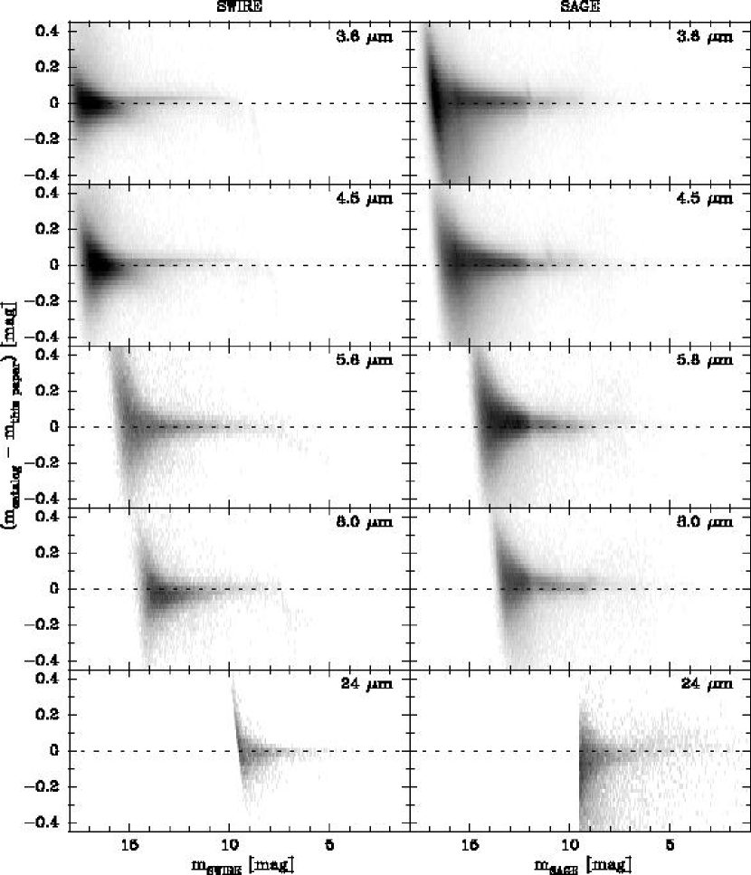
Figure 1: Comparison with photometric results from the SWIRE and SAGE catalogs. The horizontal axis of the panels in the left column use the measurements from the SWIRE DR2 and DR3 catalogs while those in the right column use the measurements from the SAGE DR1 catalog. The vertical axis shows the difference between the catalog values and our measurements.

The results from comparison of our photometric measurements with those of the SWIRE and SAGE surveys are shown in Figure 1. We find reasonable agreement with both surveys. The SWIRE survey has used the SExtractor software (Bertin & Arnouts, 1996) to obtain their photometric measurements. None of the apertures used for source extraction by the SWIRE team are identical to those used for our LMC work so we have chosen to make a comparison with their results obtained with a slightly larger aperture (4$\farcs$1 vs. our 3$\farcs$6 aperture) to minimize any effect that might arise from slight differences in the aperture locations relative to the source centroid.

The photometric measurements released by SAGE were obtained by using a modified version of the IRAF routine DAOPHOT (Stetson, 1987) that was developed to process data of the GLIMPSE Legacy Program (Benjamin et al., 2003). Similar to this work sources were initially identified using DAOFIND, however, less restrictive sharpness and roundness criteria were used ($0.2\geq sharpness\geq 1.2$ and $-1.5\geq roundness\geq 1.5$; private communication B. Babler). Cosmic-ray hits were rejected in subsequent processing steps (a more detailed description is available on the GLIMPSE and SAGE websites: http://www.astro.wisc.edu/glimpse and http://sage.stsci.edu/). Unlike the simple aperture extraction used for both SWIRE and this work, the SAGE analysis uses PSF-fitting which enables photometric estimates even in crowded fields.

In order to further quantify these comparisons for each of the IRAC bands and the MIPS 24 $\mu$m band, Table 3 lists: N_λ, the number of measurements in common with SWIRE and SAGE; $\Delta_{\lambda}$, the median offset of our measurements from those made by SWIRE and SAGE in magnitudes; and $\sigma_{\lambda}$, the root mean squared (rms) dispersion around the median offset in magnitudes. Our results show small systematic offsets of a few hundreths of a magnitude when compared to those obtained by SWIRE and SAGE. These systematic offsets appear to grow larger as we approach and exceed our completeness limits (see § 3.2). Our results appear to better match those of SWIRE, as the comparison with the SAGE results generally have a larger dispersion. This is not surprising as the SWIRE photometric extraction method is similar to ours and the SWIRE observations generally do not suffer from crowding. Based on the results in Figure 1 and Table 3 differences as large as 20% between our flux measurements and those made by the SAGE team could be expected; however, our photometric results should be adequate to identify YSOs.

3.2 Completeness and Crowding

We have constructed luminosity functions for each IRAC and MIPS band for the entire LMC (see Figure 2). We find that our source counts peak at 16.6, 16.0, 14.3, 13.1, and 9.4 mag for 3.6, 4.5, 5.8, 8.0, and 24 $\mu$m, respectively. To estimate the completeness limits for our IRAC and MIPS 24 $\mu$m photometry we have randomly placed test sources with varying brightness throughout the original IRAC and MIPS post-BCD images. We then searched for these test sources using the same software that was used for our original search. The test sources were created using the IRAC and MIPS point response functions (PRFs) with 1/5 pixel sampling available on the Spitzer Science Center website. For the IRAC, the PRF shape changes as a function of its position on the array and 25 different PRFs are available. In order to accommodate this varying PRF we alternated among the 25 IRAC PRFs using a different PRF for each test source. When adding a test source to an image we also include Poisson noise to reflect the photon statistics for the new source. We note that this additional noise is a slight over-estimate but should only make a minor difference except for the faintest test sources.

The SAGE survey mapped the central 7${}^{\circ}\times$7^∘ area of the LMC at two epochs. At each epoch the IRAC portion of the survey is composed of 49 fields that are $\sim$1.35 square degrees each. Similarly, the MIPS 24 $\mu$m portion of the survey at each epoch is composed of 38 strips, taken in the scan map mode, which have a width of $\sim$27′ and cover $\sim$2.05 square degrees each. These observations produced 98 post-BCD images for each IRAC band and 78 post-BCD images for each MIPS band and make up the majority of the observations used in our analysis.

We randomly placed 1000 test sources with a constant brightness in each of the post-BCD images from the SAGE survey. Only 1000 sources were added at a time so that the number density of sources in the image would not change significantly. We then used the same IRAF scripts to identify and extract sources. The results were then checked to determine whether or not the test sources were detected. Our software which merged the individual photometric catalogs from each post-BCD image made cross-checks among the resulting lists. These checks were designed to both remove cosmic-ray hits and to double check sources that were not identified in all possible observations. To test this portion of our algorithm, test sources in an overlapping region of multiple images are placed at the same sky positions in each of these images. A test source was deemed “found” or “recovered” if it was found in any of the images and not rejected by the cross-check. This tends to increase our detection rate near the completeness limit because marginal cases have multiple chances to be identified and then reconfirmed in the cross-check stage.

The entire process was repeated for sources with brightnesses spanning the range of those detected in the survey and was repeated for all the IRAC and MIP 24 $\mu$m images that made up the SAGE survey. This results in a total of 98,000 test sources for each brightness level in each of the IRAC bands and 78,000 test sources in the MIPS 24 $\mu$m band. These trials made up the main body of our search and enables an estimate of the overall completeness trends when considering the entire LMC.

In order to investigate the effects of crowding and bright diffuse emission on the completeness limits, we recorded the number of sources within 1′ of each test source and the RMS of the background prior to adding the test source. Note that a direct comparison to the local background is not possible because the photometry was carried out using post-BCD products which contain background offsets and gradients. To have sufficient statistics to make a meaningful comparison in regions with either a high number density of sources and/or bright diffuse emission it was necessary to make additional tests using a few images that contained these rarer conditions.

Figure 3 shows the results of our analysis of the completeness limits. When considering the LMC survey region as a whole the 90% completeness limits are 16.0, 15.0, 14.3, 13.1, and 9.2 mag at 3.6, 4.5, 5.8, 8.0, and 24 $\mu$m, respectively. These values are similar to or slightly brighter than those implied by the peaks in the source luminosity functions (Figure 2). In the most crowded regions, those with a source density of $>$24 arcmin^-2 at 3.6 and 4.5 $\mu$m, the completeness limits drop by roughly 1 mag. Less than 0.5% of the survey region has such number densities. At 5.8, 8.0, and 24 $\mu$m the source number densities rarely exceed 16, 8, and 4 arcmin^-2, respectively. Figure 3 appears to suggest that even such low number densities change the completeness limits at 24 $\mu$m, but this really results from higher background emission which generally occurs in star forming regions where the 24 $\mu$m source number densities are highest.

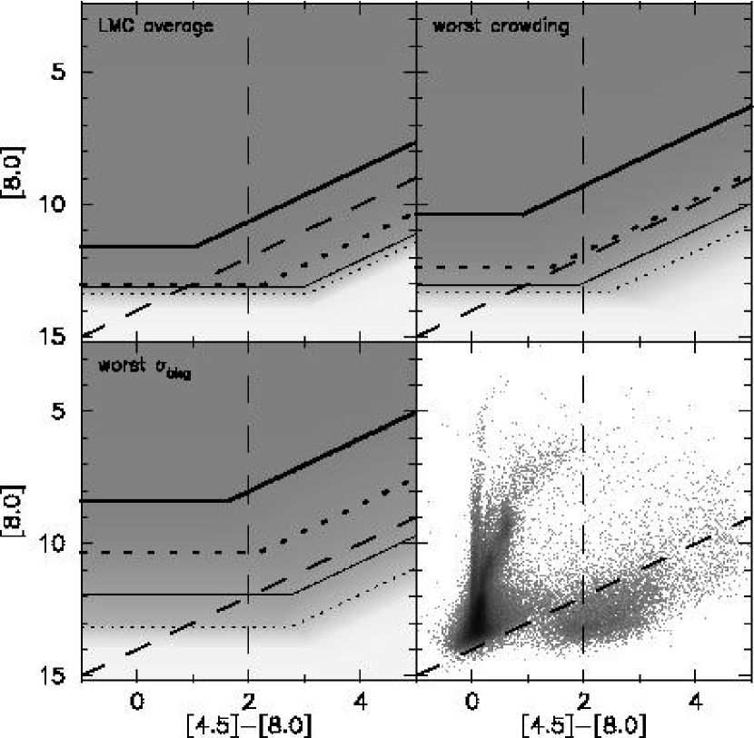
Figure 4: Completeness results in the initial color-magnitude space used to select YSO candidates. The thick solid lines mark the limit for 99% completeness while the thick dotted, thin solid, and thin dotted lines mark the limits for 90%, 75%, and 50% completeness, respectively. The heavy dashed lines mark the cutoffs that define our initial YSO sample. The top left panel shows the completeness limits when considering the entire LMC survey area. The top right and bottom left panels show the completeness limits under the “worst” crowding and background conditions we were able to probe. The bottom right panel shows the [8.0] vs. [4.5]$-$[8.0] Hess diagram of the LMC for comparison.

Examination of the completeness results as a function of the RMS background shows the extent to which a higher background will impair our ability to identify sources. At the highest RMS background levels that we could probe statistically ($\sim$5–10 MJy sr^-1) we found that the 90% completeness limits dropped by $\sim$3 mag. While these regions again make up less than 0.5% of the survey region they are most likely to occur amid bright dust emission and therefore may be associated with the YSO candidates. Figure 4 demonstrates how the completeness limits compare with the color-magnitude space used to identify our initial sample of YSOs (see § 4). We estimate that this initial YSO sample will begin to become incomplete for [8.0]$>$8.0.

To further investigate whether our aperture photometry may suffer some incompleteness for sources closer than $\sim$3″ due to crowding; we have compared our luminosity functions for three $\sim$1°$\times$1° regions in the LMC with those constructed from the SAGE DR1, which should suffer less from crowding since the photometry was obtained using PSF fitting. The three regions are located (1) in the north-east portion of the LMC covering the northern half of the supergiant shell LMC-4 which contains numerous stellar associations, (2) in the LMC bar at a position where the highest surface density of sources is seen, and (3) in the south-west portion of the LMC in a modest stellar density environment. The comparisons, in Figure 5, show that in most regions our source counts are roughly similar to those found in the SAGE DR1, but in regions such as the LMC bar where crowding becomes significant we may miss many faint sources, particularly at 3.6 and 4.5 $\mu$m. Furthermore, in the LMC bar region we find a clear discrepancy at 24 $\mu$m where the luminosity functions generated from our photometry and the SAGE DR1 appear shifted in brightness by roughly 1 magnitude with respect to each other.

In order to better understand the discrepancy between our 24 $\mu$m photometry and those in the SAGE DR1 results, we have examined the location of sources as a function of the difference between our photometry and the SAGE results. We find that the sources with larger differences are generally located in regions with significant diffuse 24 $\mu$m emission. Furthermore, the larger differences occur for sources projected amid the brightest diffuse emission or within filamentary 24 $\mu$m emission. In such cases our background annulus (between 15-23″ radius, to avoid the Airy rings in the MIPS 24 $\mu$m PSF) could often under estimate the background level resulting in an overestimate for the source flux. To explore whether a closer background measurement might remove this discrepancy we repeated the aperture photometry measurements on the MIPS 24 $\mu$m observations using a 6″ radius source aperture and a background aperture between 6″ and 12″ radius (which covers the first Airy ring in the MIPS 24 $\mu$m PSF). The aperture correction for such measurements, based on our analysis of bright isolated sources, is 2.114. We find that aperture photometry performed with a closer sky annulus decreased, but did not eliminate, the discrepancy with the SAGE DR1 results, and furthermore new discrepancies arose where previously there were none. We conclude that our measurement at 24 $\mu$m may sometimes be overestimated for sources amid strong diffuse 24 $\mu$m emission.

4 Identification of Candidate YSOs in the LMC

YSOs are still enshrouded in dust that absorbs the stellar radiation and irradiate at IR wavelengths; thus, they can be identified by observed IR excesses. Theoretical predictions of YSOs in color-magnitude diagrams (CMDs) and color-color diagrams (CCDs) are usually used to compare with observations in order to assess the evolutionary stages of YSOs. Low- and intermediate-mass YSOs are known to be surrounded by circumstellar accretion disks and envelopes, and their evolution is well established; thus, models of their SEDs can be generated and predictions of their locations in CMDs and CCDs can be made (e.g., Allen et al. 2004). However, the circumstellar structure and evolution of massive YSOs are much less certain (e.g., Zinnecker & Yorke, 2007; Cesaroni et al., 2007). To identify massive YSOs, either YSO models of low-mass stars are adopted (e.g., Jones et al., 2005) or YSO models for massive stars are generated with the assumption that massive YSOs have circumstellar envelope and disk structures similar to their low-mass counterparts (e.g., Whitney et al., 2004; Robitaille et al., 2006). The SAGE team has identified YSOs by using the latter massive YSO models to predict locations of YSOs in different combinations of CMDs, and using known evolved stars, planetary nebulae, and other contaminants to mark regions in the CMDs to avoid (Whitney et al., 2008).

To carry out an independent search for YSOs, we adopt a totally different approach. We start by examining mid-IR CMDs and CCDs for the LMC and SWIRE data, and decide to adopt the [8.0] vs. [4.5]$-$[8.0] CMD as the starting point to separate YSOs from foreground and background contaminants, in agreement with the suggestion of Harvey et al. (2006). We use this CMD to select YSO candidates first, then examined more closely each of the candidate and considered the source morphology, environment, and spectral energy distribution (SED) over as wide a wavelength range as possible to better assess their nature.

4.1 Methodology: Minimizing Contaminants

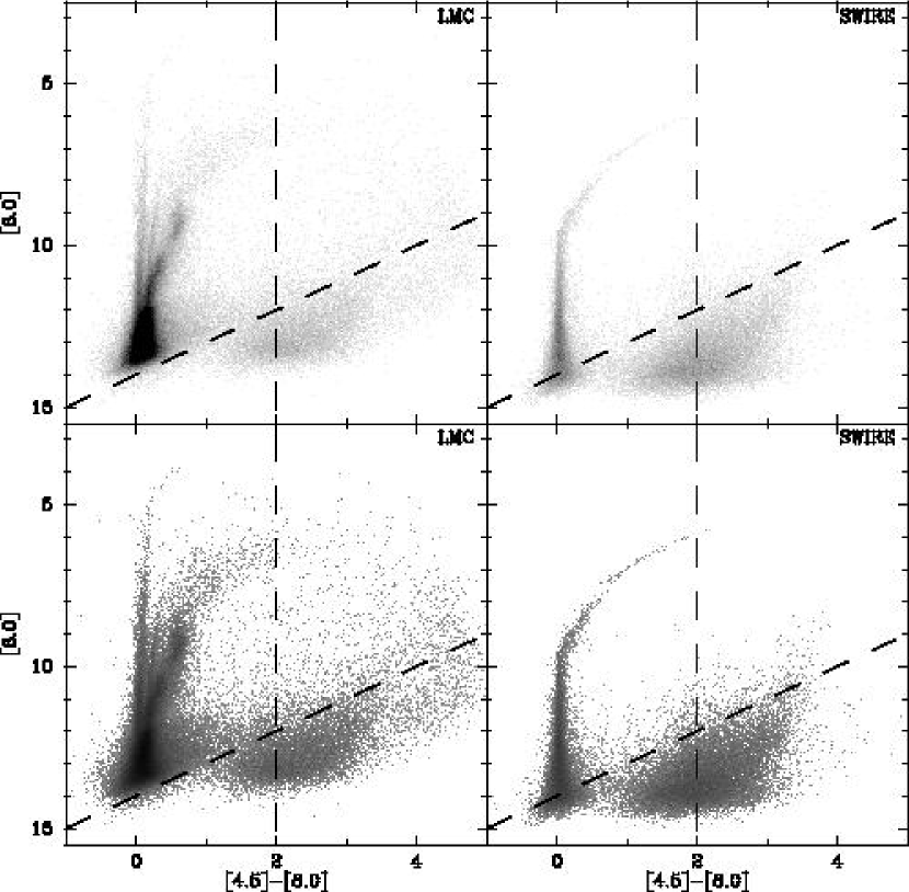
Figure 6: Color-magnitude diagrams using IRAC [8.0] vs. [4.5]$-$[8.0] for the LMC (left panels) and the SWIRE survey (right panels) shown as Hess diagrams. The panels in the top row use a square-root stretch while those in the bottom row use a logarithmic stretch to make both sharp features and the broad range covered by sources clear. The vertical dashed line marks the cutoff used to exclude most AGB, post-AGB, and main sequence stars (predominantly to the left), while the diaganol dashed line marks the criteria used to exclude background galaxies (below this cutoff). Note that points with $[8.0]\gtrsim 5.0$ in the LMC survey and $[8.0]\gtrsim 9.0$ in the SWIRE survey are saturated.

In Figure 6 we present CMDs showing the IRAC 8.0 $\mu$m flux with respect to the [4.5]$-$[8.0] color for all sources in the LMC and SWIRE fields as Hess diagrams. In these CMDs, main sequence stars will appear near [4.5]$-$[8.0]$\simeq$0 while stars on the red giant branch (RGB) and asymptotic giant branch (AGB) form the features which branch to the right of the main sequence due to excess mid-IR emission arising from the dust in their stellar winds. Examples of known LMC objects in similar CMDs have been presented for massive stars (Bonanos et al., 2009) and AGB stars (Blum et al., 2006). In the [8.0] vs. [4.5]$-$[8.0] CMD, YSOs are also expected to lie to the right of the main sequence as they are surrounded to varying degrees by the dusty remains of the protostellar core from which they formed (e.g., Allen et al., 2004; Robitaille et al., 2006).

To better understand the area over which AGB stars might be present in this CMD we consider their expected colors and luminosities based on models for Galactic C- and O-rich AGB stars by Groenewegen (2006). While the LMC has a lower metallicity, AGB atmospheric models depend on the stellar synthesized C and O abundances more than the initial abundances, thus the Galactic models are adequate in providing a rough range of colors for the LMC AGB stars. These models predict that most AGB stars have [4.5]$-$[8.0]$<$2 but that some rarer deeply enshrouded AGB stars redder than [4.5]$-$[8.0]$=$2 should be expected. Thus, we have used [4.5]$-$[8.0]$>$2.0 as the first criterion to exclude AGB stars, main-sequence stars, and giants from our sample. Recent analysis of the SAGE data by Blum et al. (2006) have confirmed that this criterion will likely exclude most C and O-rich AGB stars but that some “extreme” AGB stars may be present in the sample. The criteria of [4.5]$-$[8.0]$>$2.0 will exclude more evolved YSOs that have dispersed most of their circumstellar dust, but we are undertaking a follow-up program to identify these evolved massive YSOs.

To illustrate the locations of background galaxies in the CMD, we use observations from the SWIRE Legacy Program, which was designed to study mid-IR properties of extragalactic sources. The six fields observed in the SWIRE survey are all at high Galactic latitudes; therefore, the two populations of objects that dominate the [8.0] vs. [4.5]$-$[8.0] CMD for the SWIRE fields will be foreground Galactic stars and background galaxies. The SWIRE CMDs in Figure 6 shows that main-sequence foreground stars at [4.5]$-$[8.0]$\simeq$0 curve toward the red for [8.0]$<$9 mag where the sources begin to saturate due to the 30 s frame time used for these observations. The remaining sources are dominated by distant galaxies. In order to exclude as many distant galaxies from our LMC data as possible but still retain as many possible YSO candidates, we use a color-magnitude cut where sources with [8.0]$>$14$-$([4.5]$-$[8.0]) are excluded (Harvey et al., 2006).

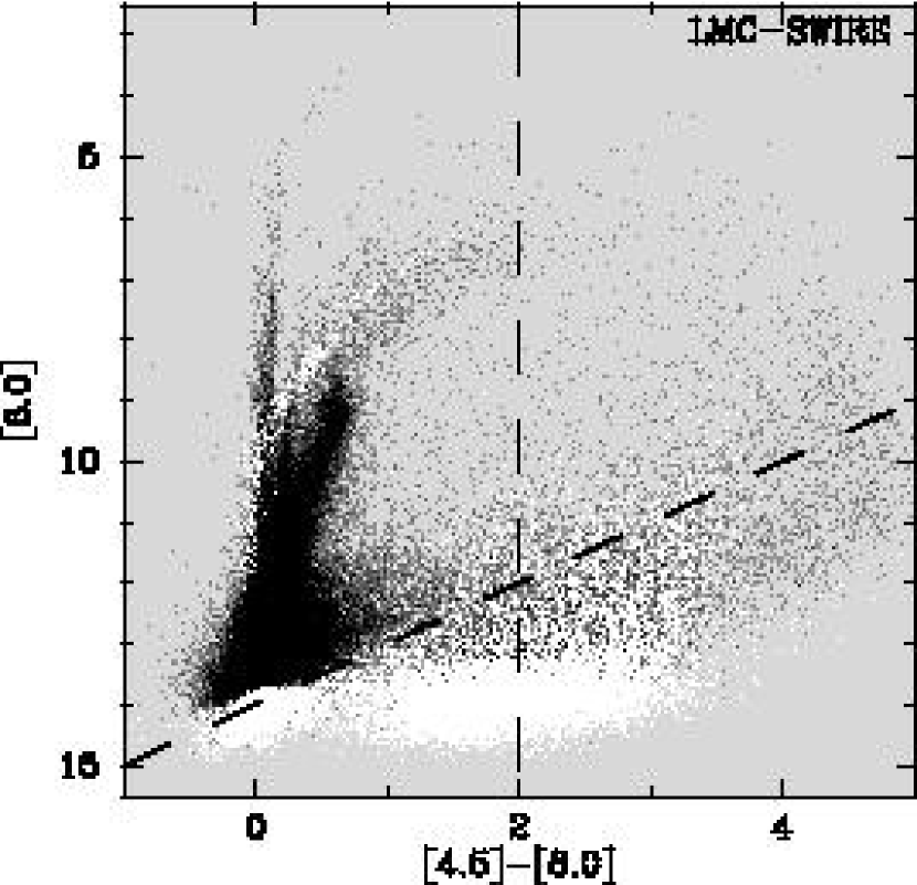
Figure 7: The difference between the LMC and SWIRE color-magnitude Hess diagrams for the [8.0] vs. [4.5]$-$[8.0] CMD after normalizing by the survey areas.

Within the wedge in the [8.0] vs. [4.5]$-$[8.0] CMD of the LMC defined by these two criteria we find 2910 sources remain. As the total extinction through the LMC is less than that for Galactic molecular clouds, from which the empirical criterion was derived (Harvey et al., 2006), we expect some background galaxies may be present in our sample. To estimate the extent to which background galaxies should be present we have examined the same wedge in the SWIRE CMD. After eliminating sources from the saturated main sequence we find 859 sources remain. We then use the 4.5 and 8.0 $\mu$m images from the SWIRE and LMC surveys to estimate the area covered and find that the total area covered by SWIRE is $\sim$48.2 square degrees while the LMC survey covers 61.7 square degrees. Assuming that both surveys are complete in this region of the CMD we estimate that $\sim$1100 background galaxies should still contaminate our initial set of candidates. Furthermore, since the SWIRE Survey data are deeper than the LMC survey data we can test whether a sample of candidate YSOs selected from the sources in this region of the CMD is affected by the completeness limits of our photometry. To do this we normalize the Hess diagrams by the area covered by the survey from which they are taken and subtract the SWIRE CMD from the LMC CMD. The resulting differenced Hess diagram is shown in Figure 7. The areas in Figure 7 where the deeper SWIRE observations consistently have more source counts appear white and demonstrate that the area of the [8.0] vs. [4.5]$-$[8.0] CMD we are using to search for YSOs should be complete excluding regions with exceptional crowding or with a complex or bright background (see Figure 4).

4.2 Methodology: Verification of YSO Candidates and Further Elimination of Contaminating Sources

4.2.1 Additional Supporting Observations

While the 2910 sources thus selected could be YSOs, among them there should still be a significant number of AGB stars, post-AGB stars, and galaxies. The LMC has been surveyed at many wavelengths and we will now combine the results from some of these other surveys to better assess the nature of the selected sources using both imaging and photometric results. We use images to assess not only the source morphology but also the surrounding interstellar environment. At the same time we use existing photometric surveys to extend the SED from the mid-IR to the near-IR and optical wavelengths.

Specifically, we have downloaded the red images from the Digitized Sky Survey (DSS2r), obtained the H$\alpha$ images from the Magellanic Clouds Emission Line Survey (MCELS; Smith et al., 1999), and downloaded the $J$, $H$, and $K_{s}$-band images from 2MASS (Skrutskie et al., 2006) for comparison with the IRAC and MIPS images. To extend the SEDs of sources we have used the near-IR photometry from the 2MASS PSC (Skrutskie et al., 2006) and the optical photometry from the Magellanic Clouds Photometric Survey (MCPS; Zaritsky et al., 2004). The 2MASS PSC has completeness limits in the absence of confusion of 15.8, 15.1 and 14.3 mag (or 0.78, 0.97, and 1.3 mJy) in the $J$, $H$, and $K_{s}$-bands, respectively. In the MCPS survey there is little evidence for incompleteness at $V<$ 20 mag ($<$36 $\mu$Jy), but the survey shows severe incompleteness at $UBVI$ of 21.5, 23.5, 23, and 22 mag (4.3, 1.8, 2.3, and 3.8 $\mu$Jy), respectively. In order to identify potential counterparts among the near-IR and optical catalogs, we cross-correlated the positions of the sources from 2MASS and MCPS with the positions of sources from our IRAC and MIPS photometry, and a positive match was considered to be closer than 1$\farcs$0. In the rare cases where an IRAC source has multiple matches in the 2MASS or MCPS catalogs, the closest near-IR/optical source is assumed to be the counterpart.

For many regions in the LMC we have obtained observations using the MOSAIC and ISPI cameras on the CTIO Blanco 4m telescope (see §2.4). These images have higher angular resolution (typically sub-arcsecond) and better sensitivity than the DSS2r or 2MASS images. Where possible we use these MOSAIC $I$-band and ISPI $J$ and $K_{s}$-band images to further supplement our analysis as they are better able to reveal fainter background galaxies, detect faint optical and near-IR counterparts to sources, and resolve groups and clusters associated with the YSO candidates.

To obtain a rough assessment of the molecular gas environment we use the available maps from the NANTEN CO(J=1-0) survey of the LMC (Fukui et al., 2001) which covers most of the area observed by Spitzer. These maps allow us to determine whether or not each source is associated with giant molecular clouds (GMCs). The NANTEN survey is sensitive to GMCs with masses greater than $\sim$1-2$\times 10^{4}$ M_⊙.

4.2.2 Multi-Wavelength Assessment of Sources

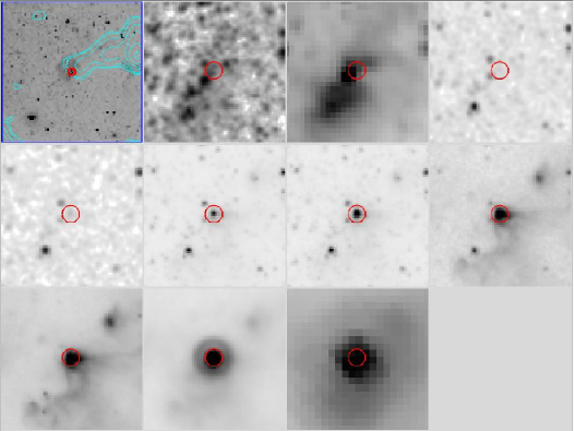
Figure 8: A screen capture showing images and plots used when classifying each candidate. The images on the left are for the source 051023.7$-$692620.2. The image in the top-left corner has a wide field to show the location within the LMC using an MCELS-H$\alpha$+continuum image overlaid with CO contours from the NANTEN survey. The remaining images show a close-up view of the source. From top-to-bottom and left-to-right those images are: DSS2r, MCELS-H$\alpha$+continuum, 2MASS-J, 2MASS-K, IRAC 3.6, IRAC 4.5, IRAC 5.8, IRAC 8.0, MIPS 24, MIPS 70. In this screen capture the wide-field image has a $\sim$20′ extent while the other panels show an $\sim$80″$\times$80″ field. The solid circle in the center of each image has a 5″ radius. The plots on the right show the spectral energy distribution for the source both as $\nu$F_ν vs. wavelength and F_ν vs. wavelength as well as the source location marked as a blue star in the [8.0] vs. [4.5]-[8.0] CMD. The DS9 utility allows changes in image contrast, magnification, and a cross-check for the alignment of the source at different wavelengths. (A color version of this figure is available in the electronic edition only.)

We used this large volume of multi-wavelength observations extending from optical to mid-IR wavelengths to assess the nature of each source in our initial sample. To this end we have constructed a library of “postage stamp” images with a field-of-view $\sim$5′$\times$5′ ($\sim$75$\times$75 pc) centered at the location of the IRAC source for wavelengths ranging from $\sim$6000 Å to 70 $\mu$m, specifically: red continuum, H$\alpha$, $J$-band, $K_{s}$-band, 3.6 $\mu$m, 4.5 $\mu$m, 5.8 $\mu$m, 8.0 $\mu$m, 24 $\mu$m, and 70 $\mu$m images. Using the flexible capabilities of DS9 (Joye & Mandel, 2003) we then simultaneously displayed and considered these postage-stamp images along with the SED based on the photometry to assess the nature of the source. In doing so we consider not only the relative source brightness in multiple wavelengths but also the source morphology, the immediate stellar and interstellar environment, and the nature of other sources in that environment. Figure 8 shows an example for one candidate of the graphical information displayed by the software used when classifying sources. We further used the SIMBAD Astronomical Database to search for previously identified sources and considered any previous assessment of their nature.

5 Results

The multi-wavelength assessment of each source was made independently by both authors and the results were compared to reach a final consensus. The resulting taxonomy splits the candidate sources into five categories: (1) evolved stars, (2) planetary nebulae, (3) background galaxies, (4) diffuse sources, and (5) definite, probable, and possible YSO candidates. Below we describe the characteristics common to most objects in each category, present a few illustrative examples, and provide tabulated lists of sources with their photometric measurements. In the following description of the common characteristics of each type of source, it should be stressed that the nature of each source is never assessed based on one single characteristic, instead it is based on a consensus of all available criteria. In many cases, particularly for fainter sources, the results of this analysis do not reach a definitive assessment as to the nature or classification of a source but instead reach a conclusion that is better described as a likelihood for the nature of a source.

5.1 AGB and post-AGB stars

In §4.1 we chose a mid-IR color criteria that would exclude most AGB and post-AGB stars based on the models of Groenewegen (2006). These models suggest that there should still exist some extreme objects which are deeply embedded in a dusty envelope that will have mid-IR colors and brightnesses consistent with our preliminary YSO source criteria. These sources can be identified when considering their images and SEDs because (1) they are typically not associated with any interstellar gas or dust structures, (2) their mid-IR SEDs peak in the IRAC bands ($<$8.0 $\mu$m) and drop in the MIPS 24 $\mu$m and 70 $\mu$m bands, and (3) their mid-IR SEDs appear roughly consistent with that of a blackbody with temperature between $\sim$400 and 1000 K. In some cases these sources show an SED with two peaks one in the optical/near-IR and one in the mid-IR similar to the SEDs of post-AGB stars with dusty tori (e.g., de Ruyter et al., 2006).

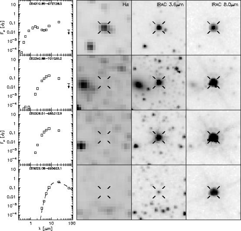
Figure 9: Examples for sources that have been identified as AGB/post-ABG stars. The panels in the left column show the SEDs for each source. The optical near-IR, and mid-IR photometry are from the MCPS, 2MASS, and this paper, respectively. Three-$\sigma$ upper limits are indicated by an arrow where applicable. To the right of each SED are images of the source at H$\alpha+$continuum (MCELS), IRAC 3.6 $\mu$m and IRAC 8.0 $\mu$m. The field of view for each image is 60″$\times$60″. The SED and images in the bottom row are for a source identified as an ERO which has no optical or near-IR counterpart. The best-fit single temperature black-body for this ERO with T=274$\pm$55 K is shown as a dashed line.

We find that roughly 111 of the 442 sources with [8.0]$<$8.0 mag to be likely either AGB or post-AGB stars, but among sources with [8.0]$>$8.0 mag only six sources that fit the same description are present. These sources appear similar to the “extreme” AGB stars noted by Blum et al. (2006). In Table High and Intermediate-Mass Young Stellar Objects in the Large Magellanic Cloud we summarize the positions, mid-IR photometric measurements, and cross-identifications with known sources using common designations from the SIMBAD database for the sources we have classified as AGB and post-AGB stars. We show four examples of sources from this category in Figure 9.

In addition to the “normal” AGB and post-AGB stars we find 13 sources with [4.5]-[8.0]$>$4 mag with no optical or near-IR counterpart in the DSS or 2MASS surveys. Eleven of the 13 sources have [8.0]$<$8.0 mag. We refer to these sources as Extremely Red Objects (EROs) as their mid-IR colors are much redder than the typical sources we identify as AGB and post-AGB stars. Their SEDs appear to peak between 8 and 24 $\mu$m and have either much lower 70 $\mu$m fluxes or are not significantly detected in the MIPS 70 $\mu$m observations. All 13 of these sources are in isolated environments, not associated with interstellar gas or dust structures. They do not appear to be concentrated toward the LMC Bar nor does their spatial distribution noticeably match that of the underlying LMC stellar distribution. These objects appear to form a unique class, although some of them have been suggested to be evolved stars or YSOs (Loup et al., 1997; Whitney et al., 2008). Subsequent IRS observations of 7 of these EROs have revealed that they are extreme carbon stars (Gruendl et al., 2008). Therefore we include these sources among those in Table High and Intermediate-Mass Young Stellar Objects in the Large Magellanic Cloud where their class is designated “E.” The bottom panel in Figure 9 shows an example of one or these sources.

5.2 Planetary Nebulae

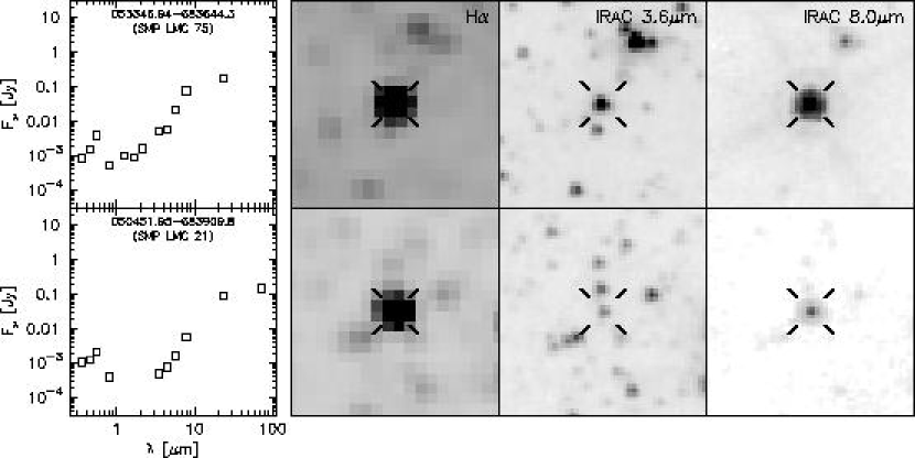
Figure 10: Examples for sources that have been identified as PNe. The panels in the left column show the SEDs for each source with images from the MCELS-H$\alpha$+continuum, IRAC 3.6 $\mu$m and IRAC 8.0 $\mu$m shown to the right.

We find that 53 of the initial sample are coincident with objects that have been previously identified as likely LMC planetary nebulae (e.g., Lindsay & Mullan, 1963; Sanduleak et al., 1978; Morgan & Good, 1992; Reid & Parker, 2006). These sources are primarily identified through our search for known counterparts but are also evident as they are generally marginally resolved or unresolved H$\alpha$ sources in the MCELS survey, and further they typically have SEDs that appear irregular, reflecting that the primary emission at different wavelengths alternate among nebular lines, PAH, and dust emission. Two examples are shown in Figures 10 and the positions, photometric measurements, and cross-identifications to known sources are summarized in Table High and Intermediate-Mass Young Stellar Objects in the Large Magellanic Cloud.

5.3 Background Galaxies

Based on comparisons with results from the SWIRE data we estimate roughly $\sim$1,100 background galaxies should be present among our initial sample of sources, and we expect this population to be evenly distributed throughout the survey area. We are able to identify these galaxies through three complementary methods.

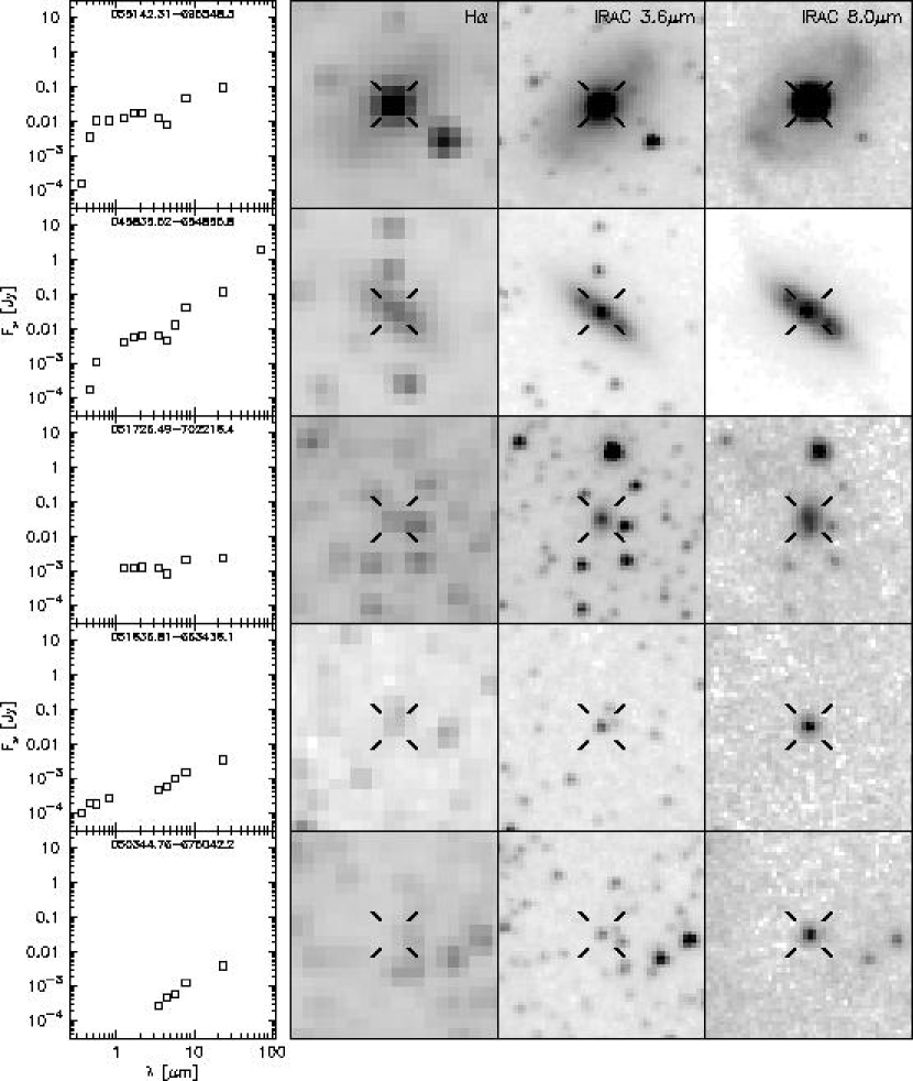
Figure 11: Similar to Figure 9 but for sources that have been identified as galaxies.

First, a large fraction of the background galaxies are easily identified by closely inspecting the images as they are extended sources (see Figure 11). In these cases the galaxy has been identified as a potential candidate in our catalog of point sources because either the galaxy is only marginally resolved or the unresolved nuclear region has been identified as a point source. Second, by examining the SED that results from these resolved and marginally resolved galaxies we are able to further identify some fainter and unresolved background galaxies with similar SEDs as is the case of the last two examples in Figure 11. Finally, there exist a set of sources with flat or slightly rising SEDs. We find that these SEDs are similar to those of known background Seyfert galaxies and quasi-stellar objects in our sample. Based on the similarity in SEDs and their being isolated from interstellar gas and dust structures, we tentatively identify these sources as background galaxies.

We have divided the background galaxies into two subsets that reflect the relative certainty of the sources being background galaxies. The first subset, “background galaxies,” are those sources which are clearly extended or which appear to be marginally resolved and have an SED that matches those of the extended sources. The second subset, “probable galaxies,” do not appear extended, are generally isolated (not associated with any interstellar structures), and have SEDs that are similar to those of either resolved galaxies or known active galaxies. We find that the range of SEDs seen among those categorized as “background galaxies” and “probable galaxies” are similar to those seen in other samples of distant galaxies observed by Spitzer (e.g., Dey et al., 2008). The positions, photometric measurements and cross-identifications with previously known objects are summarized for these sources in Tables High and Intermediate-Mass Young Stellar Objects in the Large Magellanic Cloud and High and Intermediate-Mass Young Stellar Objects in the Large Magellanic Cloud. We find 959 and 116 sources that are categorized as background galaxies and probable background galaxies, respectively. As this matches the prediction of 1,100 background galaxies to within a few percent we expect that the contamination by unidentified background galaxies in our final sample of YSO candidates should be minimal. We caution that this should not be interpreted to mean that the classification of any individual object as a background galaxy is correct.

5.4 Diffuse Sources

We have found a moderate contamination among our initial sample by “sources” that are local enhancements within filamentary dust emission most notably at either intersections between filaments or at sharp bends in filaments. We refer to these as “diffuse sources.” Diffuse sources are identified through careful inspection of the images, particularly through comparison of the IRAC images where the sources were identified, and searches for counterparts in the near-IR and MIPS images. When such a feature appears to be an enhancement in a filament and no evidence for a counterpart to the local enhancement in the IRAC bands is seen at longer or shorter wavelengths, we place the source in the diffuse category. In searching for near-IR counterparts to an IRAC source, the ISPI $J$ and $K_{s}$-band images, which are typically 2-3 mag deeper than the 2MASS Survey have proven to be powerful tools as they place a strong limit to the existence of a near-IR counterpart.

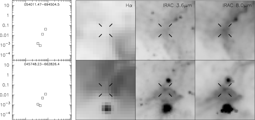
Figure 12: Similar to Figure 9 but for candidates that have are diffuse “sources” (see § 5.4 for an explanation).

A total of 159 sources were classified as diffuse. In the examples shown in Figure 12 we see that these “sources” typically exhibit a mid-IR SED indicative of PAH emission (e.g., Jones et al., 2005; Gorjian et al., 2004). Although these are most likely local peaks in the interstellar dust emission rather than true point sources, we summarize their locations and properties in Table High and Intermediate-Mass Young Stellar Objects in the Large Magellanic Cloud. Note that these diffuse sources might contain low- or even intermediate-mass YSOs as HST NICMOS images of a few diffuse sources in the 30 Dor region have revealed Herbig Ae/Be stars and lower mass pre-main-sequence stars (Brandner et al., 2001).

5.5 Young Stellar Objects

Both images and the SED of each source are critical in the identification of YSOs as these sources can have distinctly different properties depending on their evolutionary state and their environment. Due to their dusty surroundings we expect YSOs to have significant mid-IR emission, but this emission and the SED at other wavelengths will vary depending on the distribution and geometry of any circumstellar disk and envelope material. Therefore, there is not a single set of criteria that describe all YSO candidates but rather a broad range that can encompass a wide variety of sources.

The YSO sources we have identified have SEDs that rise in the mid-IR between 3.6 and 8.0 $\mu$m, which is not surprising due to the initial criteria that [4.5]$-$[8.0]$>$2.0. Furthermore, most YSO candidates have counterparts in the MIPS 24 $\mu$m images (note that in some cases no photometric measurement is available at 24 $\mu$m due to crowding, saturation, or the presence of bright diffuse emission). In many cases we find that YSO candidates have near-IR and sometimes even optical counterparts but these can reflect the evolutionary stages of the candidates or whether there are deeper ISPI and MOSAIC images available.

We have divided the YSO candidates into three groups that reflect our confidence as to their true nature: (1) “Definite YSOs” where we are highly confident of their nature, (2) “Probable YSOs” where some characteristic of the source points to a possible alternative nature, such as a background galaxy, and (3) “Possible YSOs” where we have a higher confidence that the source is not a YSO but cannot definitively rule out that the source is a YSO. The third group of sources, possible YSOs, are included for completeness so that these sources are not summarily dismissed from further consideration of their true nature.

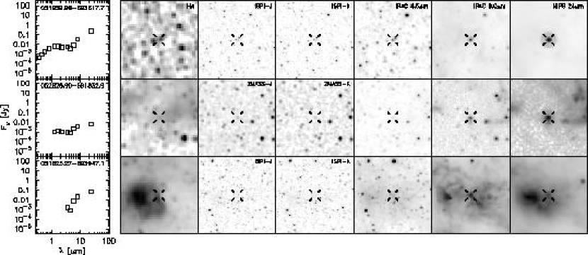
Figure 15: Similar to Figure 13a but for candidates that have been classified as “Possible.” From top to bottom the rows show the SEDs and images of 051959.98$-$693617.7, 052825.90$-$691832.9, 051823.27$-$693947.1, which are respectively examples of the SC, GC, and DC classes.

In Figures 13–15 we show examples from all three groups of sources. Furthermore, Figures 13b-–x and Figures 14b&c present SEDs and images for all 247 sources classified as definite or probable YSOs with [8.0]$<$8 and are available in the electronic edition of the Journal. In general, sources in our first two groups, definite and probable YSOs, have a clear 24 $\mu$m counterpart, and the brighter sources also have a 70 $\mu$m counterpart. The sources in the third group, possible YSOs, tend to be among the fainter sources where 24 $\mu$m and 70 $\mu$m counterparts could lie below the detection threshold or are more easily hidden amid diffuse emission. Among the original 2910 candidates 855 have been classified as definite YSOs, 317 as probable YSOs, and 213 as possible YSOs. The positions and photometric measurements of the definite, probable, and possible YSOs are summarized in Tables High and Intermediate-Mass Young Stellar Objects in the Large Magellanic Cloud–High and Intermediate-Mass Young Stellar Objects in the Large Magellanic Cloud, respectively.

5.6 Resulting Classification System

Using the above broad categories each source in our initial sample was assigned a class based on each author’s assessment. For the brightest sources (those with [8.0]$<$8), both authors classified each source on two different occasions. For the fainter sources, the first author went through the classification process for all sources twice. These results were then intercompared and synthesized to obtain a final classification for each source. The classes for AGB/post-AGB stars, EROs, PNe, background galaxies, diffuse sources, and candidate YSOs were respectively designated with A, E, P, G, D, and C. In order to accommodate the degree of certainty that a source fit into a class, the option was given to suggest a secondary or alternate class for each source. For example, a source that was most likely a YSO candidate but had many characteristics that suggested its true nature might still be a background galaxy would be classified with the designation CG and would fall into the broad category of Probable YSO. On the other hand, if the source was most likely a galaxy but a YSO candidate could not be ruled out the designation would have been GC and the source would be included in the both the probable galaxy class and in the possible YSO class. Consequently, such a source would appear in both the table of probable background galaxies (Table High and Intermediate-Mass Young Stellar Objects in the Large Magellanic Cloud) and in the table of possible YSOs (Table High and Intermediate-Mass Young Stellar Objects in the Large Magellanic Cloud). Figure 14a shows sources classified as probable YSOs and has examples of sources with a CG classification while Figure 15 shows sources classified as possible YSOs and has an example of a source in the GC class.

In our analysis, two other broad classes were needed to accommodate a number of sources. The first of these were “normal” stars, which include objects exhibiting normal stellar photospheric emission and excess mid-IR emission due to circumstellar dust. These sources were designated with “S.” The positions and photometric measurements of the 293 sources we have classified as stellar are summarized in Table High and Intermediate-Mass Young Stellar Objects in the Large Magellanic Cloud. The sources in Table High and Intermediate-Mass Young Stellar Objects in the Large Magellanic Cloud are dominated by three classifications: 64 “normal” stars (class S), 165 stars with photometric contamination from diffuse emission (class SD), and 39 stars with an IR excess that could possibly be YSOs (class SC). The second broad class consists of rejected sources. These are generally sources near the edge of the survey region where incomplete sets of observations prohibit proper classifications. There are a few other cases where unrejected transients (e.g., cosmic ray hits) had resulted in faulty photometric measurements and hence source SED. These sources were designated “R” and are not among the tabulated sources.

A follow-up Spitzer IRS program (PID: 40650) obtained observations of 269 of our brighter, definite and probable YSOs. The first results from this program show that $\gtrsim$95% of these objects have mid-IR spectra in the range between $\sim$5–37 $\mu$m consistent with our assessment that they are YSOs (Seale et al., 2009). The YSOs candidates included in this IRS survey included most of those with [8.0]$<$8.0 mag but did not extend to sources fainter than [8.0]=9.0 mag. Therefore, we conclude that a majority of the brighter YSOs candidates reported here are indeed YSOs.

6 Discussion

Using the results from our multi-wavelength assessment of YSO candidates it is now possible to examine the observed properties of the sources with respect to the classification we have made. In Table 13 we summarize the number of objects that have been assigned into each class described in the previous section. In this section we examine the spatial and photometric properties of the sources and compare our results to those of the SAGE team.

6.1 The Spatial Distribution of Red Mid-IR sources in the LMC

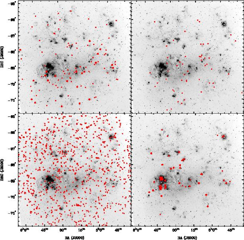
Figure 16: Each panels shows the MCELS H$\alpha$+continuum image of the LMC overlaid with the positions of sources that have been excluded from our sample of candidate YSOs. The positions of evolved stars (top left), planetary nebulae (top right), background galaxies (bottom left), and diffuse sources (bottom right) are marked with red filled circles when the nature of the source is relatively more certain and red open circles if their classification should be considered questionable.

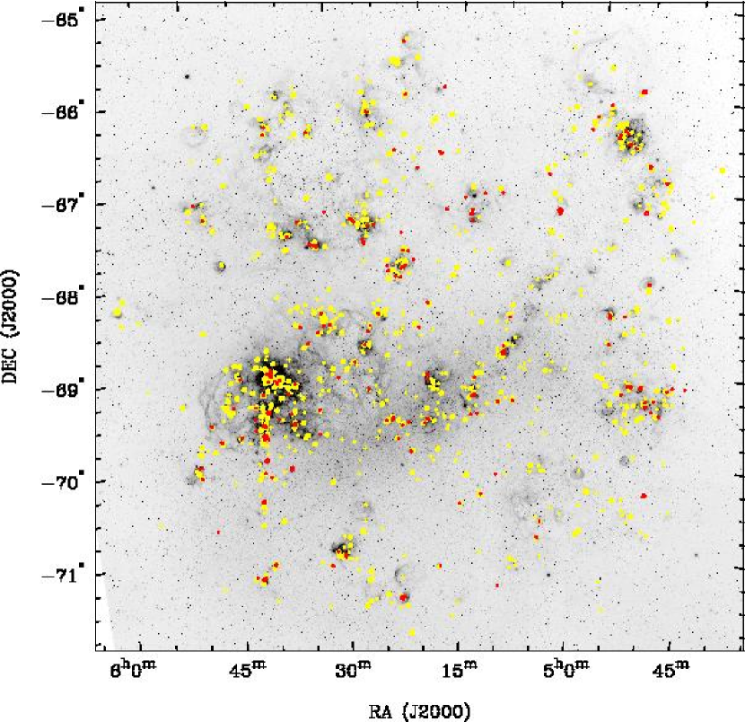
Figure 17: MCELS H$\alpha$+continuum image of the LMC overlaid with positions of candidate YSOs. Sources shown with red symbols have [8.0]$<$8.0 mag roughly indicating more massive YSO candidates while the remaining YSO candidates are shown with yellow symbols. Solid circles mark the locations of source classified as “Definite YSOs,” open circles mark “Probable YSOs,” and crosses mark “Possible YSOs.”

Figures 16 and 17 show the location of sources with different classes throughout the LMC. The AGB/post-AGB stars and PNe populations will be incomplete but do appear more concentrated toward the LMC center as expected if they follow the underlying stellar distribution. In contrast the background galaxies appear randomly distributed across the field while the diffuse sources are concentrated in regions with high H$\alpha$ surface brightness. The distribution of background galaxies is consistent with a homogeneous population of distant sources. Similarly, the diffuse sources tend to lie in and around H II regions consistent with our appraisal that these faux sources are knots in dusty nebular material. Furthermore, the relatively higher UV radiation field in the vicinity of the H II regions provides a natural explanation for why the SEDs often appear to be dominated by emission from PAHs.

In Figure 17 the sources we have classified as definite, probable, and possible YSOs show a completely different distribution. They tend to be concentrated in or around either molecular clouds or H II regions. Moreover, this tendency becomes more pronounced if the candidates classified as possible YSOs are excluded. This implies that the YSOs are roughly correlated with the concentrations of dense gas or regions where active massive star formation took place within the last few Myr. This latter association demonstrates that star formation rarely takes place as a single event but rather is extended in the time domain.

We note that those sources classified as possible YSOs should generally be excluded when analyzing the overall star formation properties in the LMC. This is in line with our description of the “possible YSO” source class as these are sources whose nature had a more likely alternate explanation but where a YSO nature was not completely excluded. We conclude that the distributions of YSO candidates along with the other source populations provide a general validation to our classification efforts.

6.2 Using Color-Color and Color-Magnitude Criteria to Classify Sources

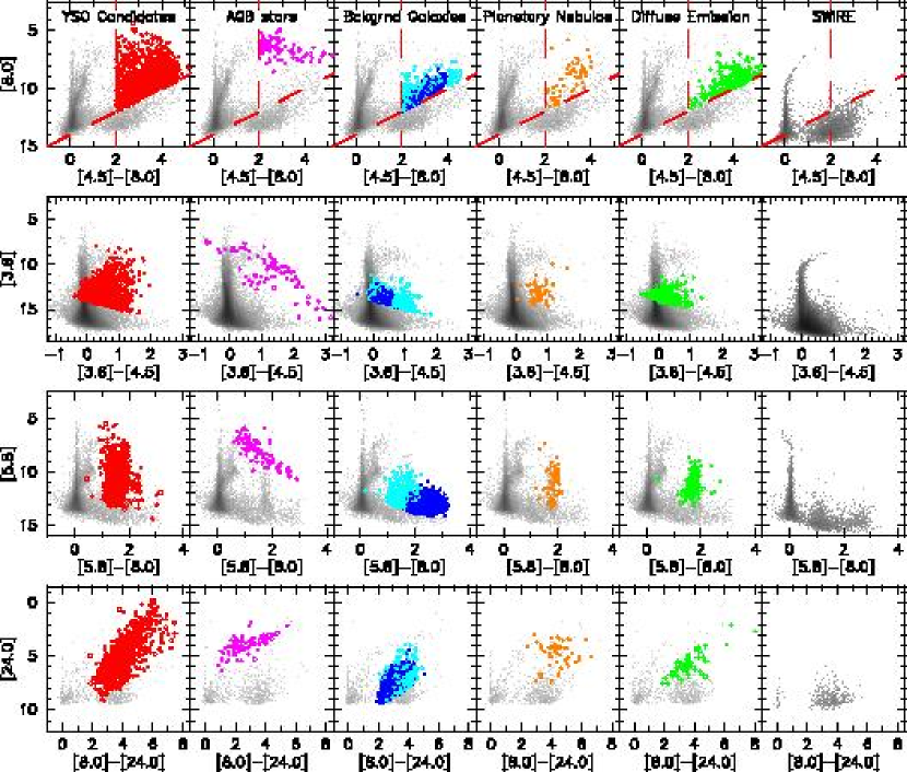
Figure 18: Each row shows a different CMD where the first five columns show a Hess diagram (greyscale) using all sources in the LMC. Each column is used for an individual source class indicated in the top row. Solid circles are used when the nature of a source was considered highly certain, open circles are used when the nature of a source is considered probable, and crosses are used to indicate points that may have a more likely explanation as to their nature. The symbols also have a color based on their class: YSOs (red), AGB stars (magenta), background galaxies (blue or cyan), PNe (orange), diffuse sources (green). For the background galaxies, the blue symbols indicate a color of [4.5]$-$[5.8]$<$[5.8]$-$[8.0]$-$1.0, and the cyan symbols show the opposite. The rightmost column in each row shows a Hess diagram derived from data in the SWIRE survey which should be dominated by Galactic stars and distant galaxies. The dashed lines in the top row show the criteria used to select the initial sample of sources.

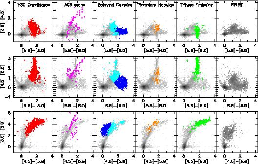
Figure 19: Same as Figure 18 but showing color-color diagrams.

We now use the source classifications to examine whether there are regions within color-color and color-magnitude space that can be combined to more effectively discriminate YSOs from the other types of sources that tend to share some photometric properties. In Figure 18 and Figure 19 we present a variety of CMDs and color-color diagrams (CCDs) for different classes of sources.

In the cases of AGB/post-AGB stars and PNe the populations suffer from small number statistics. Based on the CMDs and CCDs in Figures 18&19 it appears that many of the AGB/post-AGB stars could be identified using a complex color criteria, but that consideration of each source SEDs would still be necessary as a final discriminant to separate all AGB and post-AGB stars from the YSOs. The PNe on the other hand appear to mix among the YSO candidates no matter what photometric properties are used. Clearly optical spectra and/or emission line imaging are necessary to discriminate PNe from YSOs.

The sources we have classified as diffuse sometimes appear to be confined to relatively small areas when their IRAC colors are considered. This is particularly true of their [5.8]$-$[8.0] color which appears to fall in an narrow range of 1.5$<$[5.8]$-$[8.0]$<$2.2 mag. As previously suggested in § 5.4 this is likely due to the dominance of PAH features and is consistent with our assessment that these are dusty knots of emission. Moreover, few of these sources have near-IR or 24 $\mu$m counterparts as they do not appear in CMDs and CCDs that include longer or shorter wavelength bands. This is clearest in the bottom row of Figure 18 where nearly all the sources are marked with either an open circle or a cross because their natures are less certain. This is perhaps a selection effect as these sources were in part classified as diffuse due to their previously mentioned lack of such near-IR and 24 $\mu$m counterparts. Higher angular resolution observations are needed for the diffuse sources to search for lower mass star formation hidden within these mid-IR knots.

In the case of background galaxies, there sometimes appears to be a separation of the sources we have classified into two populations. This is most clearly evident in the [4.5]$-$[5.8] vs. [5.8]$-$[8.0] diagram in Figure 19. One of these populations, those with [4.5]$-$[5.8]$<$[5.8]$-$[8.0]$-$1.0, appear to form a distinct group that can be excluded from being YSOs based upon their mid-IR colors. We have re-examined the SEDs of the sources classified as background galaxies and find that the two populations follow the spectral classes found in § 5.3 and shown in Figure 11. Both groups are visible in the SWIRE data supporting our conclusion that both are extragalactic sources. Furthermore, based on the results of Donley et al. (2008) the group that can not be easily separated from the YSO population is likely dominated by AGN and obscured AGN.

Overall, we find that such diagrams cannot be used to unambiguously determine the nature of an individual source. It may yet be possible to determine a probability for the nature of a source from a combined analysis of all sources in multiple CMDs and CCDs. This cannot be achieved using the results of our current analysis because the only portion of color-magnitude space that has been completely analyzed is the wedge between our initial selection criteria in the [8.0] vs. [4.5]$-$[8.0] CMD.

6.3 Comparison with Star Formation Results from the SAGE Team Analysis

The SAGE collaboration has recently identified YSO candidates in the LMC using much of the same raw data we analyzed in this work (Whitney et al., 2008). The SAGE YSOs are initially identified using a complex set of color and magnitude criteria based on the predictions from a grid of radiative transfer models that attempt to simulate the emission from YSOs (Whitney et al., 2003a, b; Robitaille et al., 2006). This initial selection resulted in 3773 candidates. These candidates were then culled by requiring a YSO to: (1) have a modest amount of diffuse 24 $\mu$m emission at its location, (2) be detected in at least three bands among the four IRAC and MIPS 24$\mu$m bands, and (3) have an SED that could not be fit by a normal stellar atmosphere model. This reduced the number of YSO candidates found by the SAGE team to 1197 which they further classified into YSOs, evolved stars, PNe and galaxies.

We have searched our photometric database for sources with positional matches within 1″ or the 1197 candidates found by the SAGE team. Table 14 summarizes the results of this comparison. Of the 1197 SAGE candidates, 1190 are included in our photometric catalog while 7 had no counterpart. Of the 1190 sources in our photometric catalog, 579 met the photometric criteria in the [8.0] vs. [4.5]$-$[8.0] CMD to be included in our initial YSO sample while the remaining 611 were excluded. We have examined the photometric properties of these 611 sources to determine why they were excluded and found: 346 were excluded because they had [4.5]$-$[8.0]$<$2.0, 200 of the remaining sources were excluded because they had [8.0]$>$14$-$[4.5]$-$[8.0], and the remaining 65 were excluded due to the absence of a flux measurement at either 4.5 $\mu$m or 8.0 $\mu$m. Therefore, $\sim$89% of these 611 sources were excluded by the criteria used to prevent AGB, normal stars, and galaxies from heavily contaminating our sample while only $\sim$11% did not have the necessary photometric measurements to be considered in our analysis.

We have further compared the classifications of the 579 sources in common between our initial YSO sample selected from the [8.0] vs. [4.5]$-$[8.0] CMD with those assigned by the analysis of the SAGE team. The results are summarized in Table 15. For cases where our classification differed we have reexamined our classification but found only a few cases where we had classified a source “S” (a star with an IR excess) or “SC” (a star with an IR excess or possibly a YSO) that might be reclassified as an evolved star or switched to a more probable YSO category. The SAGE team had four classes which include the majority of their YSO candidate sources: YSO_hp (high probability YSOs), YSOs, evolved stars, and PNe. If we compare the sources classified as YSO_hp with our results we find that $\sim$76% are present in one of our three groups of YSOs but only $\sim$63% are present among the definite or probable YSOs. Similarly, for the sources in the SAGE YSO class, we find $\sim$69% are present among our three YSO groups and only $\sim$61% are present among our definite and probable YSOs. For those sources classified as YSOs by the SAGE team, our analysis has concluded that $\sim$4 to 12% are likely to be evolved stars and $\sim$20 to 33% are likely background galaxies according to our criteria. We find better agreement for sources Whitney et al. (2008) classified as evolved stars and PNe, where we classify only $\sim$15% of the evolved stars and $\sim$30% of the PNe differently.

While the similarities are encouraging, the discrepancies between our results and those of the SAGE analysis point to possible problems with both surveys. In order to restrict the number of sources we had to classify, our analysis currently ignores many sources with [4.5]$-$[8.0]$<$2.0 and many very red sources with [8.0]$>$14$-$([4.5]$-$[8.0]). The first cutoff may ignore many YSOs that are in the later stages of their evolution. Similarly, the second cutoff leaves a portion of color-magnitude space with [4.5]$-$[8.0]$>$3.5, that does not appear to have a significant number of contaminating galaxies based on the results from the SWIRE survey but which likely contains many fainter (and presumably less massive) YSOs. On the other hand, the Whitney et al. (2008) sample appears to be contaminated by background galaxies by as much as 33%. In many of these cases we are certain of our diagnosis as the source was extended in multiple bands. We suggest that the root of this problem is that the integrated SEDs of galaxies will generally show some star formation and thus can often be well fit by SED models in the libraries constructed by Robitaille et al. (2006). The discrepancies among the sources classified as PNe by the SAGE analysis may be due to the use of PN catalogs that include many sources that have not yet been spectroscopically confirmed (e.g., Reid & Parker, 2006). Follow-up spectroscopic observations should be able to discern the true nature of these sources. The closest match we find between the two samples are among the evolved stars with $\sim$85% concordance but there appears to be a fundamental discrepancy among the sources we classified as EROs which Whitney et al. (2008) have always identified as YSOs.

The largest difference between the SAGE catalog of YSOs in Whitney et al. (2008) and those presented in this paper is that we have identified 603 definite YSOs and 250 probable YSOs that do not appear in the SAGE YSO catalog. Expressed differently, the SAGE YSO catalog misses $\sim$73% of our YSOs. This cannot be explained by the color criteria used in the analysis by Whitney et al. (2008) as it includes a broader portion of color–magnitude space. Furthermore, if we look at the brightness of the sources missed by Whitney et al. (2008), we find that the percentage of sources missed remains roughly constant (between $\sim$70 and 80%) over the brightness range of $5<[8.0]<12$ mag. Chen et al. (2009) have analyzed the population of YSOs in the N 44 region and find a similar percentage of sources missing from the Whitney et al. (2008) catalog. By comparing their source lists to the original SAGE photometry catalog, they conclude that many sources are excluded from the SAGE photometric catalog because of either a higher signal–to–noise ratio threshold or a stricter requirement for a point-source morphology. The latter of these two possibilities is more consistent with our finding that the fraction of sources missed throughout the LMC does not vary with the brightness of the sources.

The photometric extraction method used for this work has allowed the inclusion of marginally extended sources and sources amid a complex interstellar background in our initial photometric catalogs. This is extremely important for uncovering the YSO population in the LMC. For Galactic searches, YSOs are generally resolved from their interstellar and even circumstellar surroundings. In the LMC, where 1″$\simeq$0.25 pc, the circumstellar and interstellar surroundings will be much harder to separate from the sources of interest. Furthermore, with the resolution afforded by Spitzer in many cases multiple YSOs are likely to be measured as a single source. Thus, relaxing the search criteria for sources is not only justified but necessary to obtain the most complete census of YSOs possible. In turn, this also requires that the individual sources be examined carefully in order to remove “diffuse” sources or local peaks in the dusty interstellar medium.

In neither the Whitney et al. (2008) analysis nor the one we present here is the YSO sample complete. Our source lists should be relatively complete for the region of the [8.0] vs. [4.5]$-$[8.0] CMD analyzed but will obviously miss sources outside that region. The Whitney et al. (2008) analysis on the other hand will provide examples of some source classes we have not analyzed; however, their more automated system of analysis appears to miss many candidates in the region of color-magnitude space we have exhaustively covered and includes sources reject as background galaxies. Studies that attempt to examine the spatial distribution of YSOs and compare with other tracers should be wary of the limitations of either YSO catalog.

6.4 Luminosity Function of our YSO Candidates

Figure 20 shows the mid-IR luminosity functions in observational units for the definite and probably YSO candidates from this paper. For the IRAC bands the distribution of brighter sources appears to roughly follow a power law until the numbers of YSO candidates begin to become incomplete due to the selection criteria that minimized the contamination by background galaxies. In the MIPS 24 $\mu$m band the luminosity function appears much different. This is because the numbers are likely incomplete over most of the plotted range where: (1) sources with [24]$\lesssim$1 will be saturated, (2) sources with [24]$\gtrsim$7.0 appear are incomplete because fainter sources are more difficult to identify amid diffuse emission, and (3) sources with [24]$\gtrsim$5.0 are likely incomplete due to the galaxy cutoff criteria.

We have assumed the rising portion of the YSO luminosity functions have a functional form $\log{N(m)}\propto\,a\,m$, where $m$ is the center of each magnitude bin, $N(m)$ is the number of sources in each bin. Least-squares fits to the luminosity functions find the slope, $a$, to range between 0.35 and 0.44 for the different IRAC bands with an average value of $\sim$0.4. The individual results are summarized in columns 2 and 3 of Table 16. In physical units the luminosity function has the form $N\propto L^{b}$, where the power law index $b$ is related to the slope $a$ by $b=-2.5~{}a$. Thus, the fitted slopes are roughly consistent with a luminosity function with power law of index $b=-1$. If we assume a mass–luminosity relation, $L\propto M^{2.4}$, for massive stars (Tout et al., 1996) and substitute this for $L$ in the luminosity function we find a mass function where $N\propto M^{-2.4}$. While this result is remarkably consistent with those found for other determinations of the initial mass function for stars with masses $\gtrsim 10~{}M_{\odot}$ (Salpeter, 1955; Miller & Scalo, 1979; Kroupa, 2001); it may also be a fortuitous coincidence as there are many potential problems in the analysis. The most notable of these are: (1) the assumption that the YSO candidates are indeed single rather than binary or multiple sources, (2) the assumption that the YSO candidates are indeed high- and intermediate mass YSOs, and (3) the unknown effect of the population of YSOs with $[4.5]-[8.0]<2.0$ that were not considered in our analysis.

The first two potential problems can be addressed by the results of a study of the YSO population in the LMC H II complex N44 by Chen et al. (2009). This study supplemented Spitzer data with optical and near-IR observations that are more sensitive and have a higher spatial resolution than typically available for our sample. They find that $\sim$60% of the N44 YSO candidates show signs in the near-IR or optical of being either extended or composed of multiple sources but that most multiples had a single source that dominates the mid-IR emission. Furthermore, they could establish whether or not the SEDs of their YSO candidates were contaminated by emission from multiple sources prior to using the models of Robitaille et al. (2006) to fit the SED. Those results indeed suggest that sources with [8.0]$<$8.0 mag are best fit with models where the central YSO has $\gtrsim$9 $M_{\odot}$ (Table 7 of Chen et al., 2009) and suggest that our candidate YSOs are indeed progenitors of high- and intermediate-mass stars. On the other hand, the fit results also demonstrate that models with a wide range of YSO masses are able to produce equally good fits to the SEDs. Thus, a mass–luminosity relationship is not strictly valid when using a single IRAC band, however, it may be a reasonable approximation when treating a large sample of YSOs.

The analysis by the SAGE team affords us a means to explore the possible contribution of sources with $[4.5]-[8.0]<2.0$ to the mid-IR luminosity function. Whitney et al. (2008) have identified 268 YSOs with $[4.5]-[8.0]<2.0$ which should not be significantly contaminated by background galaxies over the brightness range where our mid-IR luminosity functions were complete. Therefore, using the flux measurements from Table 2 of Whitney et al. (2008) we have supplemented our sample of YSOs to test whether there are significant changes to the fitted slopes ($a$). Using the same brightness ranges as above we find only small changes for the fitted value of $a$ (columns 4 and 5 of Table 16) and no change for the average value. Therefore, if the SAGE YSOs with $[4.5]-[8.0]<2.0$ are at least a representative population then the exclusion of YSOs with $[4.5]-[8.0]<2.0$ should not have significantly affected the slopes of the YSO luminosity functions.

7 Summary

We have used Spitzer IRAC and MIPS observations to obtain mid-IR photometric measurements of $>$3.5 million sources in the LMC. Comparison between the results from our photometry for the LMC and SWIRE survey with those of the SAGE and SWIRE teams, respectively, indicate that our measurements have roughly the same accuracy and completeness. We have used the mid-IR photometry to search for high- and intermediate-mass YSOs in the LMC and have identified a sample of 2,910 sources for further consideration.

Subsequent analysis using images and photometry at optical, near-IR and mid-IR wavelengths have identified a sample of 1,172 definite and probable YSO candidates along with 213 other sources for which a YSO nature could not be definitively excluded. In the process of identifying the YSOs we have also cataloged 117 objects which are likely obscured AGB stars and 1075 objects that are most likely background galaxies.

Using our classification of sources we have shown that there are no simple diagnostics in color–magnitude space that can be used to uniquely separate this population of YSOs in the LMC from background galaxies, PNe, or AGB stars. Comparison with the analysis performed on the same dataset by the SAGE team (Whitney et al., 2008) has found that this previous analysis may be contaminated at a level of roughly 20–30% by background galaxies and misses over 850 YSO candidates in the region where their analysis overlaps ours in color-magnitude space. A simple analysis of the mid-IR luminosity function of the YSOs suggest that the mass function of YSOs has a power-law index of $-$2.4, consistent with a Salpeter mass function, but it may simply be a fortuitous coincidence that this value is similar to determinations of the stellar IMF for massive stars in the Solar Neighborhood.

Clearly the nature and masses of these candidate YSOs must be better established before they can be used to rigorously study the star formation process or establish an independent estimate of the YSO mass-function in the LMC. To this end, Spitzer program 40650 has recently obtained follow-up mid-IR spectroscopic observations of 269 of the brighter definite and probable YSO presented in this paper and confirm that $\gtrsim$95% of these sources are indeed YSOs (Seale et al., 2009). Further follow-up observations with Herschel should allow better estimates of the source masses and evolutionary states. Deep, high-resolution, near- and/or mid-IR observations will enable an accurate assessment of the multiplicity of these YSO candidates and enable a search for associated lower-mass star formation.

Figure 2: Luminosity functions constructed using our IRAC and MIPS 24 $\mu$m measurements for the entire LMC survey area. In each panel a dashed line marks the brightness where saturation should begin to significantly affect the photometry of bright sources. A dotted line is used to indicate the rough brightness where we switch between the long and short exposures taken in the high dynamic range mode. A solid line marks the the expected brightness for a point source to be detected with 10$\sigma$ significance using the SAGE survey data.

Figure 3: The results from our detailed completeness tests. For each band two panels are shown plotting completeness vs. source magnitude. The heavy solid line in each panel indicates the average completeness when considering the entire LMC survey area equally. The top panels for each band show completeness as a function of crowding while the bottom panels show completeness as a function of RMS background. The alternating solid and dotted lines each represent a factor of 2 increase in number density of sources (ranging from 4–32 arcmin^-2 at 3.6 and 4.5 $\mu$m, 1–16 arcmin^-2 at 5.8 $\mu$m, 1–8 arcmin^-2 at 8.0 $\mu$m, and 1–4 arcmin^-2 at 24 $\mu$m) or a factor of 2 increase in RMS background (ranging from 0.05–6.4 MJy sr^-1 at 3.6 and 4.5 $\mu$m, 0.1–6.4 MJy sr^-1 at 5.8, 8.0 and 24 $\mu$m).

Figure 5: Luminosity functions for the IRAC and MIPS 24 $\mu$m bands from three $\sim$1 square degree regions in the LMC. Results from our photometry are shown as filled circles while those from the SAGE DR1 release are shown with open circles. The SW region (top panels), Bar region (center panels), and NE region (bottom panels) are centered at 4^h58^m,$-$70°30′  5^h21^m,$-$69°30′  and 5^h34^m,$-$66°30′  respectively. The SW and NE regions have a lower density of sources and less mid-IR nebular emission when compared to the Bar region.

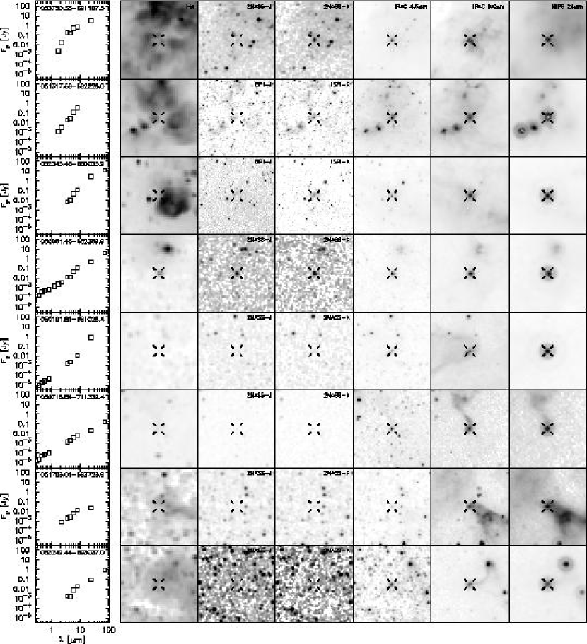
Figure 13a: A few examples of YSO candidates that have been classified as “Definite.” The panels in the left column show the SEDs for each source. The images in each row are MCELS-H$\alpha$+continuum, 2MASS-J (or ISPI-J if available), 2MASS-K (or ISPI-K if available), IRAC 4.5 $\mu$m, IRAC 8.0 $\mu$m, and MIPS 24 $\mu$m (from left to right) and show a 2^′ field of view centered on the source (marked). Figures 13b-–x present SEDs and images for all 233 sources classified as definite YSOs with [8.0]$<$8 and are available in the electronic edition of the Journal.

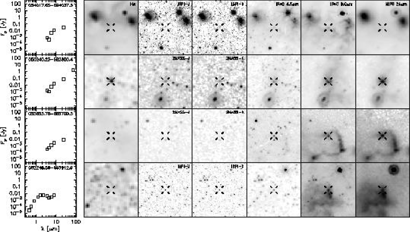
Figure 14a: Similar to Figure 13a but for YSO candidates that have been classified as “Probable.” From top to bottom the rows show the SEDs and images of 054017.65$-$694037.3, 050240.23$-$682800.4, 053653.78$-$665700.3, and 052248.56$-$693912.9, which are respectively examples of sources in the CD, CG, CG, and CS classes. Figures 14ab&c present SEDs and images for the 14 sources classified as probable YSOs with [8.0]$<$8 and are available in the electronic edition of the Journal.

Figure 20: Luminosity functions for the IRAC and MIPS 24 $\mu$m band constructed using the sources identified as definite or probable YSOs. Open symbols indicate measurements that were used to fit the slope for the brighter sources while filled symbols indicate measurements that were excluded when fitting. The best fit for each of the IRAC bands has been plotted as a dashed line.

Table 1: Observation Summary

Program	Principle		Typical Observation Parameters
ID	Investigator	Region(s)	IRAC	MIPS
Observations Used for Photometry and Imaging
124	Gehrz	N 159, N 160	10$\times$12s
1032	Brandl	30 Dor	3$\times$12s
1061	Gorjian	N 206	3$\times$12s
3565	Chu	N 11, N 44, N 51, N 63	5$\times$30s	Med Scan
		N 70, N 144, N 180
20203	Meixner	SAGE Legacy Program	4$\times$12s	2$\times$Fast Scan
Observations Used for Imaging Only
34	Fazio	AB Dor	5$\times$30s
63	Houck	30 Dor	3$\times$12s
118	Werner	5 MACHO Events	24$\times$30s
124	Gehrz	SN 1987A	64$\times$12s
		N 49	50$\times$2s
125	Fazio	LMC Bar	4$\times$12s
249	Indebetouw	LMC-C and LMC-S fields		Fast Scan
717	Rieke	N 206		Med Scan
3400	Rich	NGC 1786, NGC 1806, NGC 1831	72$\times$12s
		NGC 1856, NGC 1866, NGC 2004
		NGC 2173, NGC 2210, NGC 2004
3483	Rho	N 132D	9$\times$30s
3578	Misselt	32 LMC Extinction Probes	3$\times$12s
3680	Borkowski	15 LMC SNRs	5$\times$30s
3725	Goudfrooij	NGC 1751, NGC 1783, NGC 1846	14$\times$100s
		NGC 1978, NGC 1987, NGC 2108
		NGC 2808

Table 2: Photometric Extraction Parameters

	Aperture	Sky	Aperture	Zero	Assumed Flux
Wavelength	Radius	Annulus	Correction	Point	Calibration
[$\mu$m]	[″]	[″]		[Jy]	Accuracy
3.6	3.6	3.6–8.4	1.124	277.5	5%
4.5	3.6	3.6–8.4	1.127	197.5	5%
5.8	3.6	3.6–8.4	1.143	116.6	5%
8.0	3.6	3.6–8.4	1.234	63.1	5%
24.0	6.0	15.0–23.0	1.798	7.14	10%
70.0	18.0	18.0–39.0	1.927	0.775	20%

Table 3: Detailed Comparison of Our Photometric Measurements with SAGE and SWIRE Results

	IRAC 3.6 $\mu$m			IRAC 4.5 $\mu$m			IRAC 5.8 $\mu$m			IRAC 8.0 $\mu$m			MIPS 24.0 $\mu$m
Range	N3.6	$\Delta_{3.6}$	$\sigma_{3.6}$	N4.5	$\Delta_{4.5}$	$\sigma_{4.5}$	N5.8	$\Delta_{5.8}$	$\sigma_{5.8}$	N8.0	$\Delta_{8.0}$	$\sigma_{8.0}$	N24.0	$\Delta_{24.0}$	$\sigma_{24.0}$
[mag]		[mag]	[mag]		[mag]	[mag]		[mag]	[mag]		[mag]	[mag]		[mag]	[mag]
Comparison with SWIRE results
5.0–6.0													12	-0.016	0.013
6.0–6.0							10	-0.109	0.026	7	-0.171	0.062	29	-0.014	0.030
7.0–8.0				9	-0.087	0.033	18	-0.045	0.030	21	-0.048	0.061	107	-0.019	0.034
8.0–9.0	27	-0.157	0.087	29	-0.046	0.044	32	-0.025	0.031	33	-0.036	0.030	591	-0.026	0.054
9.0–10.0	66	-0.052	0.078	73	-0.021	0.058	70	-0.021	0.040	84	-0.032	0.047	937	-0.009	0.074
10.0–11.0	165	-0.017	0.052	152	-0.003	0.041	155	-0.020	0.040	227	-0.039	0.103
11.0–12.0	329	-0.006	0.053	336	-0.009	0.047	359	-0.019	0.064	663	-0.052	0.096
12.0–13.0	718	-0.011	0.063	718	-0.014	0.068	778	-0.026	0.106	1903	-0.062	0.073
13.0–14.0	1389	-0.016	0.073	1496	-0.019	0.076	1617	-0.029	0.129	4142	-0.057	0.107
14.0–15.0	3425	-0.029	0.073	4343	-0.036	0.080	4198	-0.027	0.195	1574	0.004	0.209
15.0–16.0	11583	-0.041	0.087	15491	-0.037	0.105	3120	0.132	0.265	6	1.023	0.731
16.0–17.0	37568	-0.029	0.118	46532	-0.016	0.152	98	0.766	0.249
17.0–18.0	45100	-0.006	0.164	17339	0.054	0.220
Comparison with SAGE results
1.0–2.0													44	-0.046	0.226
2.0–3.0													111	-0.004	0.221
3.0–4.0							10	-0.007	0.047	15	0.000	0.046	264	0.005	0.315
4.0–5.0							23	0.003	0.020	37	0.007	0.073	457	-0.007	0.299
5.0–6.0				36	0.001	0.059	81	0.004	0.124	155	0.010	0.148	838	-0.024	0.327
6.0–7.0	163	0.019	0.078	134	-0.002	0.165	269	0.022	0.187	607	0.010	0.132	1586	-0.061	0.375
7.0–8.0	440	0.021	0.209	655	0.000	0.284	1063	0.023	0.216	1168	0.013	0.189	3468	-0.094	0.366
8.0–9.0	1764	0.013	0.248	1958	0.003	0.205	1927	0.013	0.166	2533	0.024	0.095	10871	-0.091	0.262
9.0–10.0	6553	0.009	0.160	5347	0.010	0.163	5768	0.000	0.088	7110	0.010	0.082	14176	-0.103	0.176
10.0–11.0	13430	0.008	0.140	12371	0.010	0.082	13847	0.003	0.102	13470	0.011	0.102
11.0–12.0	27605	-0.002	0.128	24797	0.001	0.110	25765	0.008	0.133	27413	0.013	0.133
12.0–13.0	91654	-0.006	0.120	84025	-0.001	0.112	87999	0.008	0.152	90055	0.015	0.131
13.0–14.0	179618	-0.015	0.158	174575	-0.005	0.157	163275	0.010	0.148	62386	0.069	0.147
14.0–15.0	352594	-0.037	0.220	335183	-0.021	0.197	107277	0.081	0.179
15.0–16.0	691393	-0.074	0.251	566721	-0.023	0.190	371	0.469	0.203
16.0–17.0	1059677	-0.018	0.200	248425	0.070	0.174

Table 4: LMC Evolved Stars

Source ID	mJ	mH	m${}_{K_{\rm s}}$	m3.6	m4.5	m5.8	m8.0	m24.0	m70.0		Cross
	[mag]	[mag]	[mag]	[mag]	[mag]	[mag]	[mag]	[mag]	[mag]	Class	Identification
043257.40$-$692633.5	$\cdots$	$\cdots$	14.32$\pm$.07	10.43$\pm$.06	8.96$\pm$.05	7.72$\pm$.06	6.60$\pm$.05	4.67$\pm$.12	$>$4.19	A	MSX LMC 1008
044827.63$-$695323.0	$\cdots$	$\cdots$	$\cdots$	10.85$\pm$.05	9.09$\pm$.06	7.84$\pm$.06	6.63$\pm$.05	4.43$\pm$.12	$\cdots$	A	MSX LMC 1137
044858.14$-$684742.2	16.11$\pm$.09	15.04$\pm$.08	14.01$\pm$.07	11.55$\pm$.05	10.42$\pm$.05	9.34$\pm$.05	8.21$\pm$.06	5.52$\pm$.13	$>$4.09	AS
044918.53$-$695314.5	12.66$\pm$.03	10.85$\pm$.03	9.43$\pm$.02	7.60$\pm$.05	8.22$\pm$.05	7.07$\pm$.05	5.62$\pm$.05	4.05$\pm$.12	$\cdots$	A	MSX LMC 1130
045128.99$-$685750.1	9.93$\pm$.02	8.62$\pm$.02	7.91$\pm$.01	7.59$\pm$.05	8.24$\pm$.05	6.78$\pm$.05	5.69$\pm$.05	3.25$\pm$.11	$>$2.84	A	MSX LMC 1190

Note. — Table High and Intermediate-Mass Young Stellar Objects in the Large Magellanic Cloud is presented in its entirety in the electronic edition of the Astrophysical Journal.

Note. — Sources marked “sat.” at 24 $\mu$m are saturated or amid saturated diffuse emission.

Table 5: LMC Planetary Nebulae

Note. — Table High and Intermediate-Mass Young Stellar Objects in the Large Magellanic Cloud is presented in its entirety in the electronic edition of the Astrophysical Journal.

Table 6: Background Galaxies

Note. — Table High and Intermediate-Mass Young Stellar Objects in the Large Magellanic Cloud is presented in its entirety in the electronic edition of the Astrophysical Journal.

Table 7: Probable Background Galaxies

Note. — Table High and Intermediate-Mass Young Stellar Objects in the Large Magellanic Cloud is presented in its entirety in the electronic edition of the Astrophysical Journal.

Table 8: Diffuse Non-Sources

Note. — Table High and Intermediate-Mass Young Stellar Objects in the Large Magellanic Cloud is presented in its entirety in the electronic edition of the Astrophysical Journal.

Table 9: Definite LMC Young Stellar Objects

Note. — Table High and Intermediate-Mass Young Stellar Objects in the Large Magellanic Cloud is presented in its entirety in the electronic edition of the Astrophysical Journal.

Note. — Sources marked “sat.” at 24 $\mu$m are saturated or amid saturated diffuse emission.

Table 10: Probable LMC Young Stellar Objects

Note. — Table High and Intermediate-Mass Young Stellar Objects in the Large Magellanic Cloud is presented in its entirety in the electronic edition of the Astrophysical Journal.

Table 11: Possible LMC Young Stellar Objects

Note. — Table High and Intermediate-Mass Young Stellar Objects in the Large Magellanic Cloud is presented in its entirety in the electronic edition of the Astrophysical Journal.

Table 12: Stellar Sources

Note. — Table High and Intermediate-Mass Young Stellar Objects in the Large Magellanic Cloud is presented in its entirety in the electronic edition of the Astrophysical Journal.

Note. — Sources marked “sat.” at 24 $\mu$m are saturated or amid saturated diffuse emission.

Table 13: Summary of Sources Classification from Our Catalog

Class	Total	m${}_{8.0\mu{\rm m}}<$8.0	Possible YSOs
Definite YSOs	855	233	$\cdots$
Probable YSOs	317	14	$\cdots$
Possible YSOs	213		213
AGB/post-AGB	117	111	0
PNe	56	9	2
Galaxy	1075	7	116
Diffuse	159	12	44
Stellar	291	45	51
Reject	40	11	$\cdots$

Table 14: Comparison between SAGE and Our Catalog

SAGE		Sources	Sources	Sources
Results		Among	Not In	Not in	Reason Not In Our Sample
		Our	Our	Our	AGB	Galaxy	both	no	no
Class	Total	Sample	Sample	Catalog	cutoff	cutoff	cutoffs	4.5$\mu$m	8.0$\mu$m
YSO_hp	458	326	131	1	122	2	1	8	0
YSO	532	161	366	5	139	184	5	32	16
Evolved	118	41	76	1	69	5	2	0	4
PN	82	49	33	0	12	20	3	2	2
Galaxy	4	1	3	0	3	0	0	0	0
other	3	1	2	0	1	0	0	1	0

Table 15: Comparison between SAGE and Our Classification

	Sources
	Among	Our Class
SAGE	Our	Definite	Probable	Possible		Background	Evolved
Class	Sample	YSO	YSO	YSO	GC	Galaxy	Star	ERO	PN
YSO_hp	326	156	51	41	31	65	6	7	0
YSO	161	86	13	13	9	29	19	1	0
Evolved	41	1	3	2	0	0	35	0	0
PN	49	6	5	1	1	0	3	0	34
Galaxy	1	0	0	1	1	0	0	0	0

Table 16: YSO Luminosity Function Fit Results

Band	$a$	$\sigma_{a}$	$a$	$\sigma_{a}$
3.6	0.43	0.02	0.39	0.03
4.5	0.35	0.02	0.35	0.03
5.8	0.40	0.04	0.41	0.04
8.0	0.44	0.02	0.45	0.02

References

- Allen et al. (2004) Allen, L. E., et al. 2004, ApJS, 154, 363
- Benjamin et al. (2003) Benjamin, R. A., et al. 2003, PASP, 115, 953
- Bertin & Arnouts (1996) Bertin, E., & Arnouts, S. 1996, A&AS, 117, 393
- Blum et al. (2006) Blum, R. D., et al. 2006, AJ, 132, 2034
- Bonanos et al. (2009) Bonanos, A. Z., et al. 2009, AJ, submitted (arXiv:0905.1328)
- Brandner et al. (2001) Brandner, W., Grebel, E. K., Barbá, R. H., Walborn, N. R., & Moneti, A. 2001, AJ, 122, 858
- Caulet et al. (2008) Caulet, A., Gruendl, R. A., & Chu, Y.-H. 2008, ApJ, 678, 200
- Cesaroni et al. (2007) Cesaroni, R., Galli, D., Lodato, G., Walmsley, C. M., & Zhang, Q. 2007, Protostars and Planets V, 197
- Chen et al. (2009) Chen, C.-H. R., Chu, Y.-H., Gruendl, R. A., Gordon, K. D., & Heitsch, F. 2009, ApJ, 695, 511
- Chu & Gruendl (2008) Chu, Y.-H., & Gruendl, R. A. 2008, ASP Conf. Series, 387, 415
- Chu et al. (2005) Chu, Y.-H., et al. 2005, ApJ, 634, L189
- de Ruyter et al. (2006) de Ruyter, S., van Winckel, H., Maas, T., Lloyd Evans, T., Waters, L. B. F. M., & Dejonghe, H. 2006, A&A, 448, 641
- Dey et al. (2008) Dey, A., et al. 2008, ApJ, 677, 943
- Donley et al. (2008) Donley, J. L., Rieke, G. H., Pérez-González, P. G., & Barro, G. 2008, ApJ, 687, 111
- Fadda et al. (2006) Fadda, D., et al. 2006, AJ, 131, 2859
- Fazio et al. (2004) Fazio, G., et al. 2004, ApJS, 154, 10
- Feast (1999) Feast, M. 1999, New Views of the Magellanic Clouds, IAU Symp. 190, 542
- Fukui et al. (2001) Fukui, Y., Mizuno, N., Yamaguchi, R., Mizuno, A., & Onishi, T. 2001, PASJ, 53, L41
- Gorjian et al. (2004) Gorjian, V., et al. 2004, ApJS, 154, 275
- Goudis & Meaburn (1978) Goudis, C., & Meaburn, J. 1978, A&A, 68, 189
- Groenewegen (2006) Groenewegen, M.A.T. 2006, A&A, 448, 181
- Gruendl et al. (2008) Gruendl, R. A., Chu, Y.-H., Seale, J. P., Matsuura, M., Speck, A. K., Sloan, G. C., & Looney, L. W. 2008, ApJ, submitted
- Hartmann et al. (2005) Hartmann, L., et al. 2005, ApJ, 629, 881
- Harvey et al. (2006) Harvey, P. M., et al. 2006, ApJ, 644, 307
- Henize (1956) Henize, K. G. 1956, ApJS, 2, 315
- Jones et al. (2005) Jones, T. J., Woodward, C. E., Boyer, M. L., Gehrz, R. D., & Polomski, E. 2005, ApJ, 620, 731
- Joye & Mandel (2003) Joye, W. A., & Mandel, E. 2003, Astronomical Data Analysis Software and Systems XII, 295, 489
- Kenyon & Hartmann (1995) Kenyon, S. J., & Hartmann, L. 1995, ApJS, 101, 117
- Kroupa (2001) Kroupa, P. 2001, MNRAS, 322, 231
- Lada (1987) Lada, C. J. 1987, in IAU Symp. 115, Star Forming Regions, ed. M. Peimbert, J. Jugaku (New York: IAU), 1
- Lindsay & Mullan (1963) Lindsay, E. M., & Mullan, D. J. 1963, Irish Astronomical Journal, 6, 51
- Lonsdale et al. (2003) Lonsdale, C. J., et al. 2003, PASP 115, 897
- Loup et al. (1997) Loup, C., Zijlstra, A. A., Waters, L. B. F. M., & Groenewegen, M. A. T. 1997, A&AS, 125, 419
- Meaburn (1980) Meaburn, J. 1980, MNRAS, 192, 365
- Meixner et al. (2006) Meixner, M. M., et al. 2006,
- Miller & Scalo (1979) Miller, G. E., & Scalo, J. M. 1979, ApJS, 41, 513
- Morgan & Good (1992) Morgan, D. H., & Good, A. R. 1992, A&AS, 92, 571
- Muller et al. (1998) Muller, G. P., Reed, R., Armandroff, T., Boroson, T. A., & Jacoby, G. H. 1998, Proc. SPIE, 3355, 577
- Nikolaev et al. (2004) Nikolaev, S., et al. 2004, ApJ, 601, 260
- Regan & Gruendl (1995) Regan, M. W., & Gruendl, R. A. 1995, Astronomical Data Analysis Software and Systems IV, 77, 335
- Reid & Parker (2006) Reid, W. A., & Parker, Q. A. 2006, MNRAS, 373, 521
- Rieke et al. (2004) Rieke, G. H., et al. 2004, ApJS, 154, 25
- Robitaille et al. (2006) Robitaille, T. P., Whitney, B. A., Indebetouw, R., Wood, K., & Denzmore, P. 2006, ApJS, 167, 256
- Salpeter (1955) Salpeter, E. E. 1955, ApJ, 121, 161
- Sanduleak et al. (1978) Sanduleak, N., MacConnell, D. J., & Philip, A. G. D. 1978, PASP, 90, 621
- Seale et al. (2009) Seale, J. P. et al. 2009, ApJ, 699, 150
- Skrutskie et al. (2006) Skrutskie, M. F. et al. 2006, AJ, 131, 1163
- Smith et al. (1999) Smith, R. C., et al. 1999, IAU Symp. 190: New Views of the Magellanic Clouds, 190, 28
- Smith et al. (2002) Smith, R. C., Rest, A., Hiriart, R., Becker, A., Stubbs, C. W., Valdes, F. G., & Suntzeff, N. 2002, Proc. SPIE, 4836, 395
- Stetson (1987) Stetson, P. B. 1987, PASP, 99, 191
- Tout et al. (1996) Tout, C. A., Pols, O. R., Eggleton, P. P., & Han, Z. 1996, MNRAS, 281, 257
- van der Bliek et al. (2004) van der Bliek, N. S., et al. 2004, Proc. SPIE, 5492, 1582
- Whitney et al. (2003a) Whitney, B. A., Wood, K., Bjorkman, J. E., & Cohen, M. 2003a, ApJ, 598, 1079
- Whitney et al. (2003b) Whitney, B. A., Wood, K., Bjorkman, J. E., & Wolff, M. J. 2003b, ApJ, 591, 1049
- Whitney et al. (2004) Whitney, B. A., et al. 2004, ApJS, 154, 315
- Whitney et al. (2008) Whitney, B. A. et al. 2008, AJ, 136, 18
- Yang et al. (2007) Yang, C.-C., Gruendl, R. A., Chu, Y.-H., Mac Low, M.-M., & Fukui, Y. 2007, ApJ, 671, 374
- Zaritsky et al. (2004) Zaritsky, D., Harris, J., Thompson, I. B., & Grebel, E. K. 2004, AJ, 128, 1606
- Zinnecker & Yorke (2007) Zinnecker, H., & Yorke, H. W. 2007, ARA&A, 45, 481