The relation between gas and dust in the Taurus Molecular Cloud

Abstract

We report a study of the relation between dust and gas over a 100 deg² area in the Taurus molecular cloud. We compare the H₂ column density derived from dust extinction with the CO column density derived from the ¹²CO and ¹³CO $J=1\to 0$ lines. We derive the visual extinction from reddening determined from 2MASS data. The comparison is done at an angular size of 200^′′, corresponding to 0.14 pc at a distance of 140 pc. We find that the relation between visual extinction $A_{\rm V}$ and $N({\rm CO})$ is linear between $A_{\rm V}\simeq 3$ and 10 mag in the region associated with the B213–L1495 filament. In other regions the linear relation is flattened for $A_{\rm V}\gtrsim$ 4 mag. We find that the presence of temperature gradients in the molecular gas affects the determination of $N({\rm CO})$ by $\sim$30–70% with the largest difference occurring at large column densities. Adding a correction for this effect and accounting for the observed relation between the column density of CO and CO₂ ices and $A_{\rm V}$, we find a linear relationship between the column of carbon monoxide and dust for observed visual extinctions up to the maximum value in our data $\simeq 23$  mag. We have used these data to study a sample of dense cores in Taurus. Fitting an analytical column density profile to these cores we derive an average volume density of about $1.4\times 10^{4}$ cm^-3 and a CO depletion age of about $4.2\times 10^{5}$ years. At visual extinctions smaller than $\sim$3 mag, we find that the CO fractional abundance is reduced by up to two orders of magnitude. The data show a large scatter suggesting a range of physical conditions of the gas. We estimate the H₂ mass of Taurus to be about $1.5\times 10^{4}$ M_⊙, independently derived from the $A_{\rm V}$ and $N({\rm CO})$ maps. We derive a CO integrated intensity to H₂ conversion factor of about 2.1$\times 10^{20}$ cm^-2(K km s^-1)^-1, which applies even in the region where the [CO]/[H₂] ratio is reduced by up to two orders of magnitude. The distribution of column densities in our Taurus maps resembles a log–normal function but shows tails at large and low column densities. The length scale at which the high–column density tail starts to be noticeable is about 0.4 pc.

1. Introduction

Interstellar dust and gas provide the primary tools for tracing the structure and determining the mass of extended clouds as well as more compact, dense regions within which new stars form. The most fundamental measure of the amount material in molecular clouds is the number of H₂ molecules along the line of sight averaged over an area defined by the resolution of the observations, the H₂ column density, $N({\rm H}_{2})$. Unfortunately, H₂ has no transitions that can be excited under the typical conditions of molecular clouds, and therefore it cannot be directly observed in such regions. We have to rely on indirect methods to determine $N({\rm H}_{2})$. Two of the most common methods are observations of CO emission and dust extinction.

Carbon monoxide (CO) is the second most abundant molecular species (after H₂) in the Universe. Observations of ¹²CO and ¹³CO together with the assumption of local thermodynamic equilibrium (LTE) and moderate ¹³CO optical depths allow us to determine $N({\rm CO})$ and, assuming an [CO]/[H₂] abundance ratio, we can obtain $N({\rm H}_{2})$. This method is, however, limited by the sensitivity of the ¹³CO observations and therefore is only able to trace large column densities. Goldsmith et al. (2008) used a 100 square degree map of ¹²CO and ¹³CO in the Taurus molecular cloud to derive the distribution of $N({\rm CO})$ and $N({\rm H}_{2})$. By binning the CO data by excitation temperature, they were able to estimate the CO column densities in individual pixels where ¹²CO but not ¹³CO was detected. The pixels where neither ¹²CO or ¹³CO were detected were binned together to estimate the average column density in this portion of the cloud.

Extensive work has been done to assess the reliability of CO as a tracer of the column of H₂ molecules (e.g. Frerking et al., 1982; Langer et al., 1989). It has been found that $N({\rm CO})$ is not linearly correlated with $N({\rm H}_{2})$, as the former quantity is sensitive to chemical effects such as CO depletion at high volume densities (Kramer et al., 1999; Caselli et al., 1999; Tafalla et al., 2002) and the competition between CO formation and destruction at low-column densities (e.g. van Dishoeck & Black, 1988; Visser et al., 2009). Moreover, temperature gradients are likely present in molecular clouds (e.g. Evans et al., 2001) affecting the correction of $N({\rm CO})$ for optical depth effects.

The H₂ column density can be independently inferred by measuring the optical or near–infrared light from background stars that has been extincted by the dust present in the molecular cloud (Lada et al., 1994; Cambrésy, 1999; Dobashi et al., 2005). This method is often regarded as one of the most reliable because it does not depend strongly on the physical conditions of the dust. But this method is not without some uncertainty. Variations in the total to selective extinction and dust–to–gas ratio, particularly in denser clouds like those in Taurus, may introduce some uncertainty in the conversion of the infrared extinction to gas column density (Whittet et al., 2001). Dust emission has been also used to derive the column density of H₂ (Langer et al., 1989). It is, however, strongly dependent on the dust temperature along the line of sight, which is not always well characterized and difficult to determine. Neither method provides information about the kinematics of the gas.

It is therefore of interest to compare column density maps derived from ¹²CO and ¹³CO observations with dust extinction maps. This will allow us to characterize the impact of chemistry and saturation effects in the derivation of $N({\rm CO})$ and $N({\rm H}_{2})$ while testing theoretical predictions of the physical processes that cause these effects.

As mentioned before, CO is frozen onto dust grains in regions of relatively low temperature and larger volume densities (e.g. Kramer et al., 1999; Tafalla et al., 2002; Bergin et al., 2002). In dense cores, the column densities of C¹⁷O (Bergin et al., 2002) and C¹⁸O (Kramer et al., 1999; Alves et al., 1999; Kainulainen et al., 2006) are observed to be linearly correlated with $A_{\rm V}$ up to $\sim$10 mag. For larger visual extinctions this relation is flattened with the column density of these species being lower than that expected for a constant abundance relative to H₂. These authors showed that the C¹⁷O and C¹⁸O emission is optically thin even at visual extinctions larger than 10 mag and therefore the flattening of the relation between their column density and $A_{\rm V}$ is not due to optical depths effects but to depletion of CO onto dust grains. These observations suggest drops in the relative abundance of C¹⁸O averaged along the line-of-sight of up to a factor of $\sim$3 for visual extinctions between 10 and 30 mag. A similar result has been obtained from direct determinations of the column density of CO–ices based on absorption studies toward embedded and field stars (Chiar et al., 1995). At the center of dense cores, the [CO]/][H₂] ratio is expected to be reduced by up to five orders of magnitude (Bergin & Langer, 1997). This has been confirmed by the comparison between observations and radiative transfer calculations of dust continuum and C¹⁸O emission in a sample of cores in Taurus (Caselli et al., 1999; Tafalla et al., 2002). The amount of depletion is not only dependent on the temperature and density of the gas, but is also dependent on the timescale. Thus, determining the amount of depletion in a large sample of cores distributed in a large area is important because it allow us to determine the chemical age of the entire Taurus molecular cloud while establishing the existence of any systematic spatial variation that can be a result of a large–scale dynamical process that lead to its formation.

At low column densities ($A_{\rm V}\lesssim$ 3 mag, $N({\rm CO})\lesssim$ 10¹⁷ cm^-2) the relative abundance of CO and its isotopes are affected by the relative rates of formation and destruction, carbon isotope exchange and isotope selective photodissociation by far-ultraviolet (FUV) photons. These effects can reduce [CO]/[H₂] by up to three orders of magnitude (e.g. van Dishoeck & Black, 1988; Liszt, 2007; Visser et al., 2009). This column density regime has been studied in dozens of lines-of-sight using UV and optical absorption (e.g. Federman et al., 1980; Sheffer et al., 2002; Sonnentrucker et al., 2003; Burgh et al., 2007) as well as in absorption toward mm-wave continuum sources (Liszt & Lucas, 1998). The statistical method presented by Goldsmith et al. (2008) allows the determination of CO column densities in several hundred thousand positions in the periphery of the Taurus molecular cloud with $N({\rm CO})\simeq 10^{14}-10^{17}$ cm^-3. A comparison with the visual extinction will provide a coherent picture of the relation between $N({\rm CO})$ and $N({\rm H}_{2})$ from diffuse to dense gas in Taurus. These results can be compared with theoretical predictions that provide constraints in physical parameters such as the strength of the FUV radiation field, etc.

Accounting for the various mechanisms affecting the [CO]/[H₂] relative abundance allows the determination of the H₂ column density that can be compared with that derived from $A_{\rm V}$ in the Taurus molecular cloud. It has also been suggested that the total molecular mass can be determined using only the integrated intensity of the ¹²CO $J=1\to 0$ line together with the empirically–derived CO-to-H₂ conversion factor ($X_{\rm CO}\equiv N({\rm H}_{2})/I_{\rm CO})$. The $X_{\rm CO}$ factor is thought to be dependent on the physical conditions of the CO–emitting gas (Maloney & Black, 1988) but it has been found to attain the canonical value for our Galaxy even in diffuse regions where the [CO]/][H₂] ratio is strongly affected by CO formation/destruction processes (Liszt, 2007). The large–scale maps of $N({\rm CO})$ and $A_{\rm V}$ also allow us to assess whether there is H₂ gas that is not traced by CO. This so-called “dark gas” is suggested to account for a substantial fraction of the total molecular gas in our Galaxy (Grenier et al., 2005).

Numerical simulations have shown that the probability density function (PDF) of volume densities in molecular clouds can be fitted by a log-normal distribution (e.g. Ostriker et al., 2001; Nordlund & Padoan, 1999; Li et al., 2004; Klessen, 2000). The shape of the distribution is expected to be log-normal as multiplicative effects determine the volume density of a molecular cloud (Passot & Vázquez-Semadeni, 1998; Vázquez-Semadeni & García, 2001). A log-normal function can also describe the distribution of column densities in a molecular cloud (Ostriker et al., 2001; Vázquez-Semadeni & García, 2001). For some molecular clouds the column density distribution can be well fitted by a log–normal (e.g. Wong et al., 2008; Goodman et al., 2009). A study by Kainulainen et al. (2009), however, showed that in a larger sample of molecular complexes the column density distribution shows tails at low and large column densities. The presence of tails at large column densities seems to be linked to active star–formation in clouds. The $A_{\rm V}$ and CO maps can be used to determine the distribution of column densities at large scales while allowing us to study variations in its shape in regions with different star–formation activity within Taurus.

In this paper, we compare the CO column density derived using the ¹²CO and ¹³CO data from Narayanan et al. 2008 (see also Goldsmith et al. 2008) with a dust extinction map of the Taurus molecular cloud. The paper is organized as follows: In Section 2 we describe the derivation of the CO column density in pixels where both ¹²CO and ¹³CO were detected, where ¹²CO but not ¹³CO was detected, as well as in the region where no line was detected in each individual pixel. In Section 3 we make pixel–by–pixel comparisons between the derived $N({\rm CO})$ and the visual extinction for the large and low column density regimes. In Section 4.1 we compare the total mass of Taurus derived from $N({\rm CO})$ and $A_{\rm V}$. We also study how good the ¹²CO luminosity together with a CO-to-H₂ conversion factor can determine the total mass of a molecular cloud. We study the distribution of column densities in Taurus in Section 4.2. We present a summary of our results in Section 5.

2. The N(H₂) map derived from ¹²CO and ¹³CO

Figure 1.— Mask regions defined in the Taurus Molecular Cloud. Mask 2 is shown in black, Mask 1 in dark gray, and Mask 0 in light gray. We also show the 156 stellar members of Taurus compiled by Luhman et al. (2006) as white circles.

In the following we derive the column density of CO using the FCRAO 14–m ¹²CO and ¹³CO observations presented by Narayanan et al. 2008 (see also Goldsmith et al. 2008). In this paper we use data corrected for error beam pick-up using the method presented by Bensch et al. (2001). The correction procedure is described in Appendix A. The correction for error beam pick–up improves the calibration by 25–30%. We also improved the determination of $N({\rm CO})$ compared to that presented by Goldsmith et al. (2008) by including an updated value of the spontaneous decay rate and using an exact numerical rather than approximate analytical calculation of the partition function. The values of the CO column density are about $\sim$20% larger than those presented by Goldsmith et al. (2008). Following Goldsmith et al. (2008), we define Mask 2 as pixels where both ¹²CO and ¹³CO are detected, Mask 1 as pixels where ¹²CO is detected but ¹³CO is not, and Mask 0 as pixels where neither ¹²CO nor ¹³CO are detected. We consider a line to be detected in a pixel when its intensity, integrated over the velocity range between 0–12 km s^-1, is at least 3.5 times larger than the rms noise over the same velocity interval. We show the mask regions in Figure 1. The map mean rms noise over this velocity range is $\sigma_{T^{*}_{\rm int}}$=0.53 K km s^-1 for ¹²CO and $\sigma_{T^{*}_{\rm int}}$=0.23 K km s^-1 for ¹³CO. The map mean signal-to-noise ratio is 9 for ¹²CO and 7.5 for ¹³CO. Note that these values differ slightly from those presented by Goldsmith et al. (2008), as the correction for error beam pick–up produces small changes in the noise properties of the data.

2.1. CO Column Density in Mask 2

2.1.1 The Antenna Temperature

When we observe a given direction in the sky, the antenna temperature we measure is proportional to the convolution of the brightness of the sky with the normalized power pattern of the antenna. Deconvolving the measured set of antenna temperatures is relatively difficult, computationally expensive, and in consequence rarely done. The simplest approximation that is made is that the observed antenna temperature is that coming from a source of some arbitrary size, generally that of the main beam, or else a larger region. It is assumed that the measured antenna temperature can be corrected for the complex antenna response pattern and its coupling to the (potentially nonuniform) source by an efficiency, characterizing the coupling to the source. This is often taken to be $\eta_{\rm mb}$, the coupling to an uniform source of size which just fills the main lobe of the antenna pattern. This was the approach used by Goldsmith et al. (2008). In Appendix A we discuss an improved technique which corrects for the error pattern of the telescope in the Fourier space. This technique introduces a “corrected main–beam temperature scale”, $T_{\rm mb,c}$. We can write the main–beam corrected temperature as

$$T_{\rm mb,c}=T_{0}\left[\frac{1}{e^{T_{0}/T_{\rm ex}}-1}-\frac{1}{e^{T_{0}/T_{bg}}-1}\right]\left(1-e^{-\tau}\right),$$ (1)

where $T_{0}$ = $h\nu/k$, $T_{\rm ex}$ is the excitation temperature of the transition, $T_{bg}$ is the background radiation temperature, and $\tau$ is the optical depth. This equation applies to a given frequency of the spectral line, or equivalently, to a given velocity, and the optical depth is that appropriate for the frequency or velocity observed.

If we assume that the excitation temperature is independent of velocity (which is equivalent to an assumption about the uniformity of the excitation along the line–of–sight) and integrate over velocity we obtain

$$\int T_{\rm mb,c}(v)dv=\frac{T_{0}C(T_{\rm ex})}{e^{T_{0}/T_{\rm ex}}-1}\int(1-e^{-\tau(v)})dv\>\>,$$ (2)

where we have included explicitly the dependence of the corrected main–beam temperature and the optical depth on velocity. The function $C(T_{\rm ex})$, which is equal to unity in the limit $T_{bg}\to 0$, is given by

$$C(T_{\rm ex})=\left(1-\frac{e^{T_{0}/T_{\rm ex}}-1}{e^{T_{0}/T_{bg}}-1}\right).$$ (3)

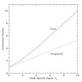
Figure 2.— Correction factors for the relation between integrated main–beam temperature and upper level column density for a Gaussian velocity distribution of the optical depth. The dotted (blue) curve shows the correction factor obtained using integrals of functions of the optical depth as given by Equation 15. The solid (red) curve shows the correction factor employing the peak values of the functions, given by Equation 16.

2.1.2 The Optical Depth

The optical depth is determined by the difference in the populations of the upper and lower levels of the transition observed. If we assume that the line–of–sight is characterized by upper and lower level column densities, $N_{U}$ and $N_{L}$, respectively, the optical depth is given by

$$\tau=\frac{h\nu_{0}}{c}\phi(\nu)\left[N_{L}B_{LU}-N_{U}B_{UL}\right],$$ (4)

where $\nu_{0}$ is the frequency of the transition, $\phi(\nu)$ is the line profile function, and the $B$’s are the Einstein B-coefficients. The line profile function is a function of the frequency and describes the relative number of molecules at each frequency (determined by relative Doppler velocity). It is normalized such that $\int\phi(\nu)d\nu$ = 1. For a Gaussian line profile, the line profile function at line center is given approximately by $\phi(\nu_{0})=1/\delta\nu_{\rm FWHM}$, where $\delta\nu_{\rm FWHM}$ is the full width at the half maximum of the line profile.

We have assumed that the excitation temperature is uniform along the line of sight. Thus, we can define the excitation temperature in terms of the upper and lower level column densities, and we can write

$$\frac{N_{U}}{N_{L}}=\frac{g_{U}}{g_{L}}e^{-T_{0}/T_{\rm ex}},$$ (5)

where the $g$’s are the statistical weights of the two levels. The relationship between the $B$ coefficients,

$$g_{U}B_{UL}=g_{L}B_{LU},$$ (6)

lets us write

$$\tau(\nu)=\frac{h\nu_{o}B_{UL}\phi(\nu)N_{U}}{c}\left[e^{T_{0}/T_{\rm ex}}-1\right].$$ (7)

Substituting the relationship between the $A$ and $B$ coefficients,

$$A_{UL}=B_{UL}\frac{8\pi h\nu_{0}^{3}}{c^{3}}\>\>,$$ (8)

gives us

$$\tau(\nu)=\frac{c^{2}A_{UL}\phi(\nu)N_{U}}{8\pi{\nu_{0}}^{2}}\left[e^{T_{0}/T_{\rm ex}}-1\right].$$ (9)

If we integrate both sides of this equation over a range of frequencies encompassing the entire spectral line of interest, we find

$$\int\tau(\nu)d\nu=\frac{c^{2}A_{UL}N_{U}}{8\pi{\nu_{0}}^{2}}\left[e^{T_{0}/T_{\rm ex}}-1\right].$$ (10)

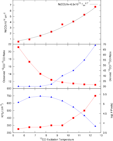
Figure 3.— Parameters of Mask 1 binned by ¹²CO excitation temperature $T_{\rm ex}$. The bottom panel shows the derived H₂ density (left-hand scale, squares) and the number of pixels in each $T_{\rm ex}$ bin (right-hand scale, triangles). The most common $T_{\rm ex}$ values are between $5-9$ K. The middle panel shows the observed (left-hand scale, squares) and derived (right-hand scale, triangles) ¹²CO/¹³CO ratio. The top panel shows the derived ¹²CO column density assuming a line width of 1 Km s^-1. The H₂ density, ¹²CO column density and derived ¹²CO/¹³CO ratio increase monotonically as a function of ¹²CO excitation temperature.

Table 1¹²CO Excitation Temperature Bins in Mask 1 and Best Estimates of Their Characteristics

$T_{\rm ex}$	12CO/13CO	Number	$n({\rm H}_{2})$	$N({\rm CO})/\delta v$	12CO/13CO
(K)	Observed	of Pixels	(cm-3)	($10^{16}$ cm-2/km s-1)	Abundance Ratio
5.5…………………..	21.21	118567	250	0.56	30
6.5…………………..	17.29	218220	275	0.95	30
7.5…………………..	14.04	252399	275	1.6	30
8.5…………………..	12.43	223632	300	2.3	32
9.5…………………..	11.76	142525	300	3.6	40
10.5………………….	11.44	68091	400	4.1	45
11.5………………….	11.20	24608	500	5.3	55
12.5………………….	11.09	6852	700	6.7	69

2.1.3 Upper Level Column Density

It is generally more convenient to describe the optical depth in terms of the velocity offset relative to that of the nominal line center. The incremental frequency and velocity are related through $dv=(c/\nu_{0})d\nu$, and hence $\int\tau(\nu)d\nu=(c/\nu_{0})\int\tau(v)dv$. Thus we obtain

$$\int\tau(v)dv=\frac{c^{3}A_{UL}N_{U}}{8\pi{\nu_{0}}^{3}}\left[e^{T_{0}/T_{\rm ex}}-1\right].$$ (11)

We can rewrite this as

$$\frac{1}{e^{T_{0}/T_{\rm ex}}-1}=\frac{c^{3}A_{UL}N_{U}}{8\pi{\nu_{0}}^{3}}\frac{1}{\int\tau(v)dv}.$$ (12)

Substituting this into Equation (2), we can write an expression for the upper level column density as

$$N_{U}=\frac{8\pi k\nu_{0}^{2}}{hc^{3}A_{UL}C(T_{\rm ex})}\left[\frac{\int\tau(v)dv}{\int(1-e^{-\tau(v)})dv}\right]\int T_{\rm mb,c}(v)dv.$$ (13)

For the calculation of the ¹³CO column densities (Section 2.1.4) we use a value for the Einstein A-coefficient of $A_{UL}=$6.33$\times 10^{-8}$ s^-1 (Goorvitch, 1994).

In the limit of optically thin emission for which $\tau(v)$ $\ll$ 1 for all $v$, and neglecting the background term in Equation (3), the expression in square brackets is unity and we regain the much simpler expression

$$N_{U}(thin)=\frac{8\pi k\nu_{0}^{2}}{hc^{3}A_{UL}}\int T_{\rm mb,c}(v)dv\>\>.$$ (14)

We will, however, use the general form of $N_{U}$ given in Equation (13) for the determination of the CO column density.

We note that the factor in square brackets in Equation (13) involves the integrals of functions of the optical depth over velocity, not just the functions themselves. There is a difference, which is shown in Figure 2, where we plot the two functions

$$CF(integral)=\frac{\int\tau(v)dv}{\int(1-e^{-\tau(v)})dv}\>\>,$$ (15)

and

$$CF(peak)=\frac{\tau_{0}}{1-e^{-\tau_{0}}}\>\>,$$ (16)

as a function of the peak optical depth $\tau_{0}$. There is a substantial difference at high optical depth, which reflects the fact that the line center has the highest optical depth so that using this value rather than the integral tends to overestimate the correction factor.

2.1.4 Total ¹³CO column densities derived from ¹³CO and ¹²CO observations.

In LTE, the column density of the upper level ($J=1$) is related to the total ¹³CO column density by

$$N_{\rm{}^{13}CO}=N_{U}\frac{Z}{(2J+1)}e^{\frac{hB_{0}J(J+1)}{KT_{\rm ex}}}$$ (17)

where $B_{0}$ is the rotational constant of ¹³CO ($B_{0}=5.51\times 10^{10}$ s^-1) and $Z$ is the partition function which is given by

$$Z=\sum^{\infty}_{J=0}(2J+1)e^{\frac{-hB_{0}(J+1)}{KT_{\rm ex}}}.$$ (18)

The partition function can be evaluated explicitly as a sum, but Penzias (1975) pointed out that for temperatures $T\gg hB_{0}/K$, the partition function can be approximated by a definite integral, which has value $kT/hB_{0}$. This form for the partition function of a rigid rotor molecule is almost universally employed, but it does contribute a small error at the relatively low temperatures of dark clouds. Specifically, the integral approximation always yields a value of $Z$ which is smaller than the correct value. Calculating $Z$ explicitly shows that this quantity is underestimated by a factor of $\sim$1.1 in the range between 8 K to 10K. Note that to evaluate Equation (18) we assume LTE (i.e. constant excitation temperature) which might not hold for high–$J$ transitions. The error due to this approximation is, however, very small. For example, for $T_{\rm ex}$=10 K, only 7% of the populated states is at $J=3$ or higher.

We can calculate the column density of ¹³CO from Equation (17) determining the excitation temperature $T_{\rm ex}$ and the ¹³CO optical depth from ¹²CO and ¹³CO observations. To estimate $T_{\rm ex}$ we assume that the ¹²CO line is optically thick ($\tau\gg 1$) in Equation (1). This results in

$$T_{\mathrm{\rm ex}}=\frac{5.53}{\ln\left(1+\frac{5.53}{T^{12}_{\mathrm{mb,c}}+0.83}\right)},$$ (19)

where $T^{12}_{\mathrm{mb,c}}$ is the peak corrected main-beam brightness temperature of ¹²CO. The excitation temperature in Mask 2 ranges from 4 to 19 K with a mean value of 9.7 K and standard deviation of 1.2 K.

Also from Equation (1), the optical depth as a function of velocity of the ¹³CO $J=1\to 0$ line is obtained from the main-beam brightness temperature using

$$\tau^{13}(v)=-\ln\left[1-\frac{T^{13}_{\mathrm{mb,c}}(v)}{5.29}\left(\left[e^{5.29/T_{\mathrm{\rm ex}}}-1\right]^{-1}-0.16\right)^{-1}\right],$$ (20)

where $T^{13}_{\mathrm{mb,c}}$ is the peak corrected main-beam brightness temperature of ¹³CO. We use this expression in Equation (15) to determine opacity correction factor. We evaluate the integrals in Equation (15) numerically. The correction factor ranges from 1 to $\sim$4 with a mean value of 1.3 and standard deviation of 0.2. The ¹³CO column density is transformed to ¹²CO column density assuming a ¹²CO/¹³CO isotope ratio of 69 (Wilson, 1999), which should apply for the well–shielded material in Mask 2.

2.1.5 Correction for Temperature Gradients along the Line of Sight

In the derivation of the CO column density and its opacity correction we made the assumption that the gas is isothermal. But observations suggest the existence of core-to-edge temperature differences in molecular clouds (e.g. Evans et al., 2001) which can be found even in regions of only moderate radiation field intensity. Therefore the presence of temperature gradients might affect our opacity correction.

We used the radiative transfer code RATRAN (Hogerheijde & van der Tak, 2000) to study the effects of temperature gradients on the determination of $N({\rm CO})$. The modeling is described in the Appendix C. We found that using ¹²CO to determine the excitation temperature of the CO gas gives the correct temperature only at low column densities while the temperature is overestimated for larger column densities. This produces an underestimate of the ¹³CO opacity which in turn affects the opacity correction of $N({\rm CO})$. This results in an underestimation of $N({\rm CO})$. We derived a correction for this effect (Equation [C2]) which is applied to the data.

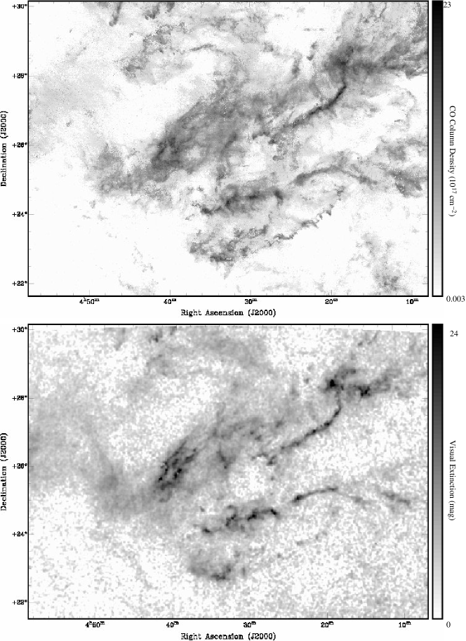
Figure 4.— Maps of the CO column density (upper panel) and visual extinction (lower panel) in the Taurus Molecular cloud. The gray-scale in the $N({\rm CO})$ and $A_{\rm V}$ maps is expressed as the square root of the CO column density and of the visual extinction, respectively. The angular resolution of the data in the figure is 40^′′ for $N({\rm CO})$ and 200^′′ for $A_{\rm V}$.

2.2. CO Column Density in Mask 1

The column density of CO in molecular clouds is commonly determined from observations of ¹²CO and ¹³CO with the assumption of Local Thermodynamic Equilibrium (LTE), as discussed in the previous section. The lower limit of $N({\rm CO})$ that can be determined is therefore set by the detection limit of the ¹³CO $J=1\to 0$ line. For large maps, however, it is possible to determine $N({\rm CO})$ in regions where only ¹²CO is detected in individual pixels by using the statistical approach presented by Goldsmith et al. (2008). In the following we use this approach to determine the column density of CO in Mask 1.

We compute the excitation temperature from the ¹²CO peak intensities for all positions in Mask 1 assuming that the emission is optically thick. The Mask 1 data is then binned by excitation temperature (in 1 K bins), and the ¹³CO data for all positions within each bin averaged together. In all bins we get a very significant detection of ¹³CO from the bin average. Thus, we have the excitation temperature and the observed ratio of integrated intensities (¹²CO/¹³CO) in each 1 K bin. Since positions in Mask 1 are distributed in the periphery of high extinction regions, it is reasonable to assume that the gas volume density in this region is modest, and thus LTE does not necessarily apply, as thermalization would imply an unreasonably low gas temperature at the cloud edges. We therefore assume that ¹²CO is sub-thermally excited and that the gas has a kinetic temperature of 15 K. We use the RADEX program (van der Tak et al., 2007), using the LVG approximation, and the collision cross sections from the Leiden Atomic and Molecular Database (LAMDA; Schöier et al., 2005), to compute line intensities. The free parameters in the modeling are temperature ($T$), density ($n$), CO column density per unit line width ($N({\rm CO})/\delta v$), and the ¹²CO/¹³CO abundance ratio ($R$). Since the excitation is determined by both density and the amount of trapping ($N/\delta v$), there is a family of $n-N({\rm CO})/\delta v$ parameters that give the same excitation temperature. The other information we have is the ¹³CO integrated intensity for the average spectrum in each bin. Thus the choice of $n$, $N({\rm CO})/\delta v$ and $R$ must reproduce the excitation temperature and the observed ¹²CO/¹³CO ratio. Solutions also must have an optical depth in the ¹²CO $J=1\to 0$ of at least 3, to be consistent with the assumption that this isotopologue is optically thick. This is the same method used in Goldsmith et al. (2008), although this time we used the RADEX program and the updated cross-sections from LAMDA.

In fact, at low excitation temperature the data can only be fit if the CO is strongly fractionated. At high excitation temperature we believe that the CO is unlikely to be fractionated, and thus, $R$ must vary with excitation temperature. We chose solutions for Mask 1 that produced both a monotonically decreasing $R$ with decreasing excitation temperature and a smoothly decreasing column density with decreasing excitation temperature. The solutions are given in Table 1 and shown Figure 3. The uncertainty resulting from the assumption of a fixed kinetic temperature and from choosing the best value for $R$ is about a factor of 2 in $N({\rm CO})$ (Goldsmith et al., 2008).

To obtain $N({\rm CO})$ per unit line width for a given value of the excitation temperature we have used a non-linear fit to the data, and obtained the fitted function:

$$\left(\frac{N({\rm CO})}{\rm cm^{-2}}\right)\left(\frac{\delta{\it v}}{\rm km\,s^{-1}}\right)^{-1}=6.5\times 10^{13}\left(\frac{T_{\rm ex}}{{\rm K}}\right)^{2.7}.$$ (21)

We multiply by the observed FWHM line width to determine the total CO column density. The upper panel in Figure 3 shows $N({\rm CO})/\delta v$ as a function of $T_{\rm ex}$.

2.3. CO Column Density in Mask 0

To determine the carbon monoxide column density in regions where neither ¹²CO nor ¹³CO were detected, we average nearly 10⁶ spectra to obtain a single ¹²CO and ¹³CO spectra. From the averaged spectra we obtain a ¹²CO/¹³CO integrated intensity ratio of $\simeq$17. We need a relatively low $R$ to reproduce such a low observed value. Values of $R=25$ or larger cannot reproduce the observed isotopic ratio and still produce ¹²CO emission below the detection threshold. Choosing $R=20$ and a gas kinetic temperature of 15 K, we fit the observed ratio with $n=100$ cm^-3 and $N({\rm CO})=3\times 10^{15}$ cm^-2. This gives rise to a ¹²CO intensity of 0.7 K, below the detection threshold, however much stronger than the Mask 0 average of only 0.18 K. Thus, much of Mask 0 must not contribute to the CO emission. In fact, only 26% of the Mask 0 area can have the properties summarized above, producing significant CO emission. Therefore, the average column density throughout Mask 0 is $7.8\times 10^{14}$ cm^-2.

Another option is to model the average spectra of ¹²CO and ¹³CO matching both the ratio and intensity. Since now, our goal is to produce CO emission with intensity 0.18 K, both ¹²CO and ¹³CO will be optically thin. Therefore we need an $R$ that is equal to the observed ratio. For $R=18$, a solution with $n=100$ cm^-3, $\delta v=1$ km s^-1, and $N({\rm CO})$ = 7.3$\times 10^{14}$ cm^-2 fits both the ¹²CO and ¹³CO average spectra for Mask 0. Note that this is very similar to the average solution (with a slightly larger $R$) that assumes that $\sim$26% of the area has column density 3$\times 10^{15}$ cm^-2 and the rest 0. Thus for a density of 100 cm^-3, the average CO column density must be about 7.8$\times 10^{14}$ cm^-2 in either model. Of course, if we picked a different density we would get a slightly different column density. As mentioned above, the uncertainty is $N({\rm CO})$ is about a factor of 2.

Note that the effective area of CO emission is uniformly spread over Mask 0. We subdivided the ¹²CO data cube in the Mask 0 region in an uniform grid with each bin containing about 10⁴ pixels. After averaging the spectra in each bin we find significant ¹²CO emission in 95% of them.

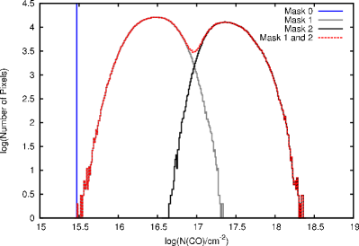
Figure 5.— Histogram of the ¹²CO column density distributions in the Mask 0, 1, and 2 regions mapped in Taurus. The Mask 0 is indicated by a vertical line at $N({\rm CO})=3\times 10^{15}$ cm^-2 which represents the column density in the CO–emitting region (26% of the area of Mask 0; see Section 2.3). Note that we have not yet corrected $N({\rm CO})$ in Mask 2 for the effect of temperature gradients in the opacity correction.

3. Comparison between A_V and $N(^{12}{\rm CO})$

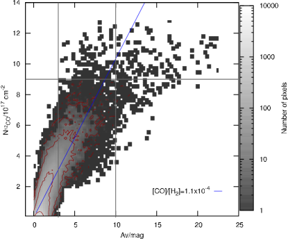
Figure 6.— Comparison between the visual extinction derived from 2MASS stellar colors and the ¹²CO column density derived from ¹³CO and ¹²CO observations in Taurus. The dark blue line represents the ¹²CO column density derived from $A_{\rm V}$ assuming $N({\rm H}_{2})/A_{\mathrm{V}}=9.4\times 10^{20}{\rm cm}^{-2}\,{\rm mag}^{-1}$ (Bohlin et al., 1978) and a [CO]/[H₂] abundance ratio of $1.1\times 10^{-4}$. The gray scale represents the number of pixels of a given value in the parameter space and is logarithmic in the number of pixels. The red contours are 2,10,100, and 1000 pixels. Each pixel has a size of 100^′′ or 0.07 pc at a distance of 140 pc.

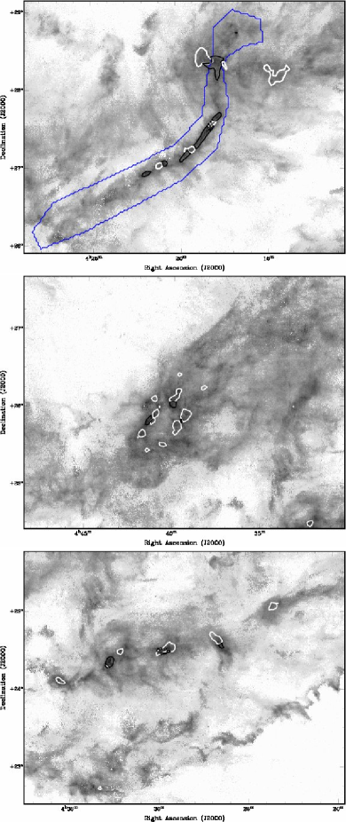
Figure 7.— $N({\rm CO})$ maps of the B213–L1495 (top), Heiles’s cloud 2 (middle), and B18–L1536 (bottom) regions. The white contours denote regions with $A_{\rm V}>10$ mag, while the black contours denote regions with $A_{\rm V}<10$ mag and $N({\rm CO})>9\times 10^{17}$ cm^-2 (see Figure 6). The blue contour outlines approximately the B213–L1457 filament.

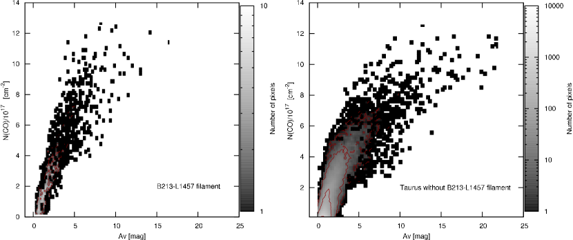
Figure 8.— Pixel–by–pixel comparison between $A_{\rm V}$ and $N({\rm CO})$ in the B213–L1457 filament (left) and the entire Taurus molecular cloud without this filament (right).

In order to test our estimate of $N({\rm CO})$ and assess whether it is a good tracer of $N({\rm H}_{2})$, we compare Mask 1 and 2 in our CO column density map of Taurus with a dust extinction map derived from 2MASS stellar colors. Maps of these quantities are shown in Figure 4. We also show in Figure 5 a histogram of the ¹²CO column density distributions in the Mask 0, 1, and 2 regions mapped in Taurus. The derivation of the dust extinction map is described in Appendix B. The resolution of the map is 200^′′ (0.14 pc at a distance of 140 pc) with a pixel spacing of 100^′′. For the comparison, we have convolved and re-gridded the CO column density map in order to match this resolution and pixel spacing.

3.1. Large $N(^{12}{\rm CO})$ Column Densities

We show in Figure 6 a pixel-by-pixel comparison between visual extinction and ¹²CO column density. The visual extinction and $N({\rm CO})$ are linearly correlated up to about $A_{\rm V}\simeq 10$ mag. For larger visual extinctions $N({\rm CO})$ is largely uncorrelated with the value of $A_{\rm V}$. In the range $3<A_{\rm V}<10$ mag, for a given value of $A_{\rm V}$, the mean value of $N({\rm CO})$ is roughly that expected for a [CO]/[H₂] relative abundance of $\sim$10^-4 which is expected for shielded regions (Solomon & Klemperer, 1972; Herbst & Klemperer, 1973). Some pixels, however, have CO column densities that suggest a relative abundance that is reduced by up to a factor of $\sim$3. In the plot we show lines defining regions containing pixels with $A_{\rm V}>10$ mag and with $3<A_{\rm V}<10$ mag and $N({\rm CO})>9\times 10^{17}$ cm^-2. In Figure 7 we show the spatial distribution of these pixels in $N({\rm CO})$ maps of the B213-L1457, Heiles’s cloud 2, and B18-L1536 regions. White contours correspond to the pixels with $A_{\rm V}>10$ mag and black contours to pixels with $3<A_{\rm V}<10$ mag and $N({\rm CO})>9\times 10^{17}$ cm^-2. Regions with $A_{\rm V}>10$ mag are compact and they likely correspond to the center of dense cores. The largest values of $N({\rm CO})$, however, are not always spatially correlated with such regions. We notice that large $N({\rm CO})$ in the $A_{\rm V}=3-10$ mag range are mostly located in the B213–L1457 filament. We study the relation between $A_{\rm V}$ and $N({\rm CO})$ in this filament by applying a mask to isolate this region (see marked region in Figure 7). We show the relation between $A_{\rm V}$ and $N({\rm CO})$ in the B213–L1457 filament in the left hand panel of Figure 8. We also show this relation for the entire Taurus molecular cloud excluding this filament in the right hand panel. Visual extinction and CO column density are linearly correlated in the B213–L1457 filament with the exception of a few pixels that are located in dense cores (Cores 3, 6 and 7 in Table 2). Without the filament the $N({\rm CO})$/$A_{\rm V}$ relation is linear only up to $\sim$4 magnitudes of extinction. In Section 3.1.1 we will see that the deviation from a linear $N({\rm CO})$/$A_{\rm V}$ relation is mostly due to depletion of CO molecules onto dust grains. Depletion starts to be noticeable for $A_{\rm V}\geq 4$ mag. Therefore, pixels on the B213–L1457 filament appear to show no signatures of depletion. This can be due either to the filament being chemically young in contrast with the rest of Taurus, or to the volume densities being low enough that desorption processes dominate over those of adsorption. If the latter case applies, and assuming a volume density of $n({\rm H}_{2})=10^{3}$ cm^-3 (low enough to not show significant CO depletion but still larger than the critical density of the ¹³CO $J=1\to 0$ line), this filament would need to be extended along the line-of-sight by 0.9–3 pc for $3<A_{\rm V}<10$ mag. This length is much larger than the projected thickness of the B213–L1495 filament of $\sim$0.2 pc but comparable to its length of $\sim$7 pc. We will study the nature of this filament in a separate paper.

Considering only regions with $A_{\rm V}<10$ mag and $N({\rm CO})>10^{17}$ cm^-2 (see Section 3.2) we fit a straight line to the data in Figure 6 to derive the [CO]/[H₂] relative abundance in Mask 2. A least squares fit results in $N({\rm CO})/{\rm cm}^{-2}=(1.01\pm 0.008)\times 10^{17}A_{\rm V}/{\rm mag}$. Assuming that all hydrogen is in molecular form we can write the ratio between H₂ column density and color excess observed by Bohlin et al. (1978) as $N({\rm H}_{2})$/E_B-V=2.9$\times 10^{21}$ cm^-2 mag^-1. We combine this relation with the ratio of total to selective extinction $R_{\rm V}=A_{\rm V}/E_{\rm B-V}\simeq 3.1$ (e.g. Whittet, 2003) to obtain $N({\rm H}_{2})/A_{\mathrm{V}}=9.4\times 10^{20}{\rm 22cm}^{-2}\,{\rm mag}^{-1}$. Combining the $N({\rm H}_{2})$/$A_{\rm V}$ relation with our fit to the data, we obtain a [CO]/[H₂] relative abundance of 1.1$\times 10^{-4}$. Note that, as discussed in Appendix B, grain growth would increase the value of $R_{\rm V}$ up to $\sim$4.5 in dense regions (Whittet et al., 2001). Due to this effect, we estimate that the derived $A_{\rm V}$ would increase up to 20% for $A_{\rm V}\leq$10 mag. This would reduce the $N({\rm H}_{2})$/$A_{\rm V}$ conversion but also increase the $A_{\rm V}$/$N({\rm CO})$ ratio. Thus the derived [CO]/[H₂] abundance is not significantly affected.

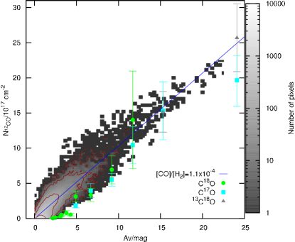
Figure 9.— The same as Figure 6 but including the estimated column density of CO and CO₂ ices. For comparison we show the relation between visual extinction and $N({\rm CO})$ derived from observations of rare isotopic species by Frerking et al. (1982) (see Appendix C) which also include the contribution for CO and CO₂ ices.

3.1.1 CO depletion

The flattening of the $A_{\rm V}$–$N({\rm CO})$ relation for $A_{\rm V}>10$ mag could be due to CO depletion onto dust grains. This is supported by observations of the pre-stellar core B68 by Bergin et al. (2002) which show a linear increase in the optically thin C¹⁸O and C¹⁷O intensity as a function of $A_{\rm V}$ up to $\sim$7 mag, after which the there is a turnover in the intensity of these molecules. This is similar to what we see in Figure 6. Note, however, $A_{\rm V}$ alone is not the sole parameter determining CO freeze-out, since this process also depends on density and timescale (e.g. Bergin & Langer, 1997).

Following Whittet et al. (2010), we test the possibility that effects of CO depletion are present in our observations of the Taurus molecular cloud by accounting for the column of CO observed to be in the form of ice on the dust grains. Whittet et al. (2007) measured the column density of CO and CO₂ ices toward a sample of stars located behind the Taurus molecular cloud. They find that the column densities are related to the visual extinction as

$$\frac{N({\rm CO})_{\rm ice}}{10^{17}[{\rm cm}^{-2}]}=0.4(A_{\rm V}-6.7),\,\,\,A_{\rm V}>6.7\,{\rm mag},$$ (22)

and

$$\frac{N({\rm CO}_{2})_{\rm ice}}{10^{17}[{\rm cm}^{-2}]}=0.252(A_{\rm V}-4.0),\,\,\,A_{\rm V}>4.0\,{\rm mag}.$$ (23)

We assume that the total column of CO frozen onto dust grains is given by

$$N({\rm CO})^{\rm total}_{\rm ice}=N({\rm CO})_{\rm ice}+N({\rm CO}_{2})_{\rm ice}.$$ (24)

Thus, for a given $A_{\rm V}$ the total CO column density is given by

$$N({\rm CO})^{\rm total}=N({\rm CO})_{\rm gas-phase}+N({\rm CO})^{\rm total}_{\rm ice}.$$ (25)

We can combine our determination of the column density of gas-phase CO with that of CO ices to plot the total $N({\rm CO})$ as a function of $A_{\rm V}$. The result is shown in Figure 9. The visual extinction and $N({\rm CO})^{\rm total}$ are linearly correlated over the entire range covered by our data, extending up to $A_{\rm V}=23$ mag. This result confirms that depletion is the origin of the deficit of gas-phase CO seen in Figure 6.

In Figure 10 we show the ratio of $N({\rm CO})^{\rm total}$ to $N({\rm CO})_{\rm gas-phase}$ as a function of $A_{{\rm V}}$, for $A_{\rm V}$ greater than 10. The drop in the relative abundance of gas-phase CO from our observations is at most a factor of $\sim$2. This is in agreement with previous determinations of the depletion along the line of sight in molecular clouds (Kramer et al., 1999; Chiar et al., 1995).

3.1.2 CO Depletion Age

In this Section we estimate the CO depletion age (i.e. the time needed for CO molecules to deplete onto dust grains to the observed levels) in dense regions in the Taurus Molecular Cloud. We selected a sample of 13 cores that have peak visual extinction larger than 10 mag and that $A_{\rm V}$ at the edges drops below $\sim$0.9 mag (3 times the uncertainty in the determination of $A_{\rm V}$). The cores are located in the L1495 and B18–L1536 regions (Figure 7). Unfortunately, we were not able to identify individual cores in Heiles’s Cloud 2 due to blending.

We first determine the H₂ volume density structure of our selected cores. Dapp & Basu (2009) proposed using the King (1962) density profile,

$$n(r)=\begin{cases}n_{c}a^{2}/(r^{2}+a^{2})&r\leq R\\ 0&r>R,\end{cases}$$ (26)

which is characterized by the central volume density $n_{c}$, a truncation radius $R$, and by a central region of size $a$ with approximately constant density.

The column density $N(x)$ at an offset from the core center $x$ can be derived by integrating the volume density along a line of sight through the sphere. Defining $N_{c}\equiv 2an_{c}\arctan(c)$ and $c=R/a$, the column density can be written

Table 2Core Parameters

Core ID	$\alpha$(J2000)	$\delta$(J2000)	$A_{{\rm V,}c}$	$a$	Radius	$n_{c}({\rm H}_{2})$	Mass	Depletion Age
			[mag]	[pc]	[pc]	[$10^{4}$ cm-3]	[M⊙]	[$10^{5}$ years]
1	04:13:51.63	28:13:18.6	22.4$\pm$0.5	0.10$\pm$0.004	2.01$\pm$0.30	2.2$\pm$0.11	307$\pm$102	6.3$\pm$0.3
2	04:17:13.52	28:20:03.8	10.7$\pm$0.3	0.19$\pm$0.021	0.54$\pm$0.12	0.7$\pm$0.09	56$\pm$43	3.4$\pm$1.5
3	04:18:05.13	27:34:01.6	12.3$\pm$1.2	0.16$\pm$0.054	0.32$\pm$0.18	1.0$\pm$0.40	29$\pm$63	1.3$\pm$3.1
4	04:18:27.84	28:27:16.3	24.2$\pm$0.4	0.13$\pm$0.005	1.27$\pm$0.08	1.9$\pm$0.07	258$\pm$52	3.8$\pm$0.2
5	04:18:45.66	25:18:0.4	9.4$\pm$0.2	0.09$\pm$0.005	2.00$\pm$0.93	1.1$\pm$0.07	110$\pm$81	10.9$\pm$0.8
6	04:19:14.99	27:14:36.4	14.3$\pm$0.6	0.12$\pm$0.010	0.89$\pm$0.15	1.3$\pm$0.12	93$\pm$47	3.1$\pm$0.6
7	04:21:08.46	27:02:03.2	15.2$\pm$0.3	0.08$\pm$0.003	1.12$\pm$0.08	1.9$\pm$0.07	90$\pm$19	2.9$\pm$0.2
8	04:23:33.84	25:03:01.6	14.4$\pm$0.3	0.11$\pm$0.004	0.93$\pm$0.07	1.4$\pm$0.06	94$\pm$23	5.1$\pm$0.3
9	04:26:39.29	24:37:07.9	15.6$\pm$0.5	0.09$\pm$0.006	1.48$\pm$0.23	1.7$\pm$0.12	143$\pm$58	2.3$\pm$0.3
10	04:29:20.71	24:32:35.6	17.2$\pm$0.4	0.13$\pm$0.006	2.48$\pm$0.39	1.3$\pm$0.07	371$\pm$127	4.5$\pm$0.3
11	04:32:09.32	24:28:39.0	16.0$\pm$0.5	0.09$\pm$0.006	3.50$\pm$2.41	1.7$\pm$0.13	347$\pm$347	3.2$\pm$0.4
12	04:33:16.62	22:42:59.6	12.2$\pm$0.5	0.08$\pm$0.007	1.66$\pm$0.64	1.5$\pm$0.14	110$\pm$82	6.3$\pm$0.7
13	04:35:34.29	24:06:18.2	12.5$\pm$0.3	0.11$\pm$0.006	1.64$\pm$0.35	1.2$\pm$0.07	145$\pm$65	2.0$\pm$0.4

$$N(x)=\frac{N_{c}}{\sqrt{1+(x/a)^{2}}}$$

$$\times\left[\arctan(\sqrt{\frac{c^{2}-(x/a)^{2}}{1+(x/a)^{2}}})/\arctan(c)\right].$$ (27)

This column density profile can be fitted to the data. The three parameters to fit are (1) the outer radius $R$, (2) the central column density $N_{c}$ (which in our case is $A_{\rm V,c}$), and (3) the size of the uniform density region $a$.

We obtain a column density profile for each core by fitting an elliptical Gaussian to the data to obtain its central coordinates, position angle, and major and minor axes. With this information we average the data in concentric elliptical bins. Typical column density profiles and fits to the data are shown in Figure 11. We give the derived parameters of the 13 cores we have analyzed in Table 2. We convert the visual extinction at the core center $A_{\rm V,c}$ to H₂ column density assuming $N({\rm H}_{2})/A_{\mathrm{V}}=9.4\times 10^{20}{\rm cm}^{-2}\,{\rm mag}^{-1}$. We use then the definition of column density at the core center (see above) to determine the central volume density $n_{c}({\rm H}_{2})$ from the fitted parameters.

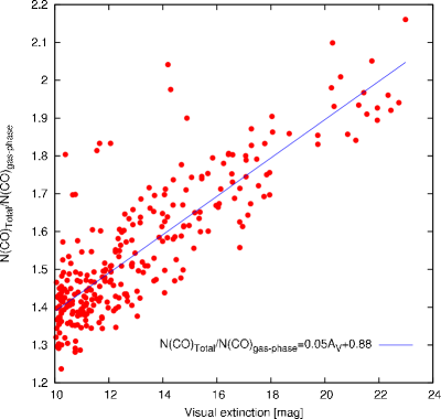
Figure 10.— Ratio of $N({\rm CO})_{\rm total}$ to $N({\rm CO})_{\rm gas-phase}$ plotted as a function of $A_{\rm V}$ for the high extinction portion of the Taurus molecular cloud. The line represents our fit to the data.

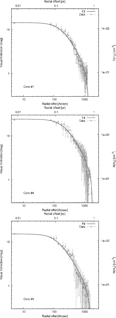
Figure 11.— Typical radial distributions of the visual extinction in the selected sample of cores. The solid lines represent the corresponding fit.

With the H₂ volume density structure, we can derive the CO depletion age for each core. The time needed for CO molecules to deplete to a specified degree onto dust grains is given by (e.g. Bergin & Tafalla, 2007),

$$t_{\rm depletion}=\left(\frac{5\times 10^{9}}{{\rm yr}}\right)\left(\frac{n({\rm H}_{2})}{{\rm cm}^{-3}}\right)^{-1}\ln(n_{0}/n_{\rm gas}),$$ (28)

where $n_{0}$ is the total gas–phase density of CO before depletion started and $n_{\rm gas}$ the gas-phase CO density at time $t_{\rm depletion}$. Here we assumed a sticking coefficient of unity (Bisschop et al., 2006) and that at the H₂ volume densities of interest adsorption mechanisms dominate over those of desorption (we therefore assume that the desorption rate is zero).

To estimate $n_{0}/n_{\rm gas}$ we assume that CO depletion occurs only in the flat density region of a core, as for larger radii the volume density drops rapidly. Then the total column density of CO (gas–phase+ices) in this region is given by $N({\rm CO})^{\rm flat}\simeq 2an_{c}(1.1\times 10^{-4})$. The gas-phase CO column density in the flat density region of a core is given by $N^{\rm flat}_{\rm gas-phase}({\rm CO})=N({\rm CO})^{\rm flat}-N({\rm CO})^{\rm total}_{\rm ice}$, where $N({\rm CO})^{\rm total}_{\rm ice}$ can be derived from Equation (25). Assuming that the decrease in the [CO]/[H₂] relative abundance in the flat region is fast and stays constant toward the center of the core (models from Tafalla et al. (2002) suggest an exponential decrease), then $n_{0}/n_{\rm gas}\simeq N({\rm CO})^{\rm flat}/N^{\rm flat}_{\rm gas-phase}({\rm CO})$. The derived CO depletion ages are listed in Table 2. Note that the fitted cores might not be fully resolved at the resolution of our $A_{\rm V}$ map (200^′′ or 0.14 pc at a distance of 140 pc). Although $n_{0}/n_{\rm gas}$ is not very sensitive to resolution, due to mass conservation, we might be underestimating the density at the core center. Therefore, our estimates of the CO depletion age might be considered as upper limits.

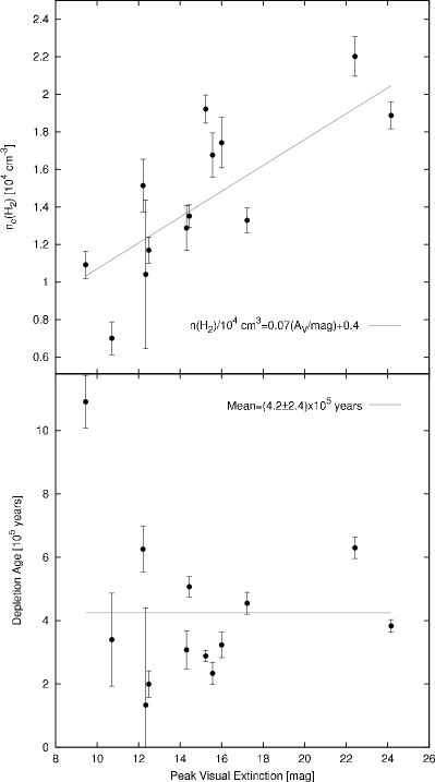
Figure 12.— (upper panel) The central H₂ volume density as a function of the peak $A_{\rm V}$ for a sample of 13 cores in the Taurus molecular cloud. The line represent a fit to the data. (lower panel) CO depletion age as a function of $A_{\rm V}$ for the sample of cores.

In Figure 12 we show the central density and the corresponding depletion age of the fitted cores as a function of $A_{\rm V}$. The central volume density is well correlated with $A_{\rm V}$ but varies only over a small range: its mean value and standard deviation are ($1.4\pm 0.4$)$\times 10^{4}$ cm^-3. Still, the moderate increase of $n({\rm H}_{2})$ with $A_{\rm V}$ compensates for the increase of $N({\rm CO})_{\rm total}/N({\rm CO})_{\rm gas-phase}$ with $A_{\rm V}$ to produce an almost constant depletion age. The mean value and standard deviation of $t_{\rm depletion}$ are $(4.2\pm 2.4)\times 10^{5}$ years. This suggests that dense cores attained their current central densities at a similar moment in the history of the Taurus molecular cloud.

3.2. Low $N(^{12}{\rm CO})$ column densities

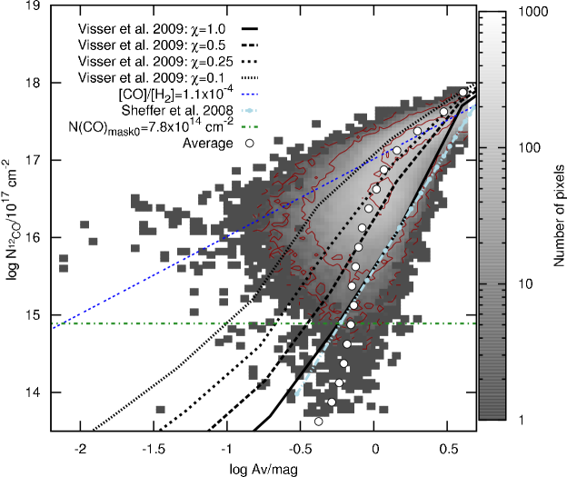
Figure 13.— Comparison between the visual extinction derived from 2MASS stellar colors and the ¹²CO column density derived from ¹³CO and ¹²CO observations in Taurus for $A_{\rm V}<5$ mag. The blue line represents the ¹²CO column density derived from $A_{\rm V}$ assuming $N({\rm H}_{2})/A_{\mathrm{V}}=9.4\times 10^{20}{\rm cm}^{-2}\,{\rm mag}^{-1}$ (Bohlin et al., 1978) and a [CO]/[H₂] abundance ratio of $1.1\times 10^{-4}$. The gray scale represents the number of pixels of a given value in the parameter space and is logarithmic in the number of pixels. The red contours are 2,10,100, and 1000 pixels. The black lines represent several models of selective CO photodissociation and fractionation provided by Ruud Visser (see text). The light blue line represents the fit to the observations from Sheffer et al. (2008) toward diffuse molecular Galactic lines-of-sight for log($N({\rm H})_{2})\geq 20.4$. The horizontal line represents the average $N({\rm CO})$ derived in Mask 0. Each pixel has a size of 100^′′ or 0.07 pc at a distance of 140 pc.

In the following we compare the lowest values of the CO column density in our Taurus survey with the visual extinction derived from 2MASS stellar colors. In Figure 13 we show a comparison between $N({\rm CO})$ and $A_{\rm V}$ for values lower than 5 magnitudes of visual extinction. The figure includes CO column densities for pixels located in Mask 1 and 2. We do not include pixels in Mask 0 because its single value does not trace variations with $A_{\rm V}$. Instead, we include a horizontal line indicating the derived average CO column density in this Mask region. We show a straight line (blue) that indicates $N({\rm CO})$ expected from a abundance ratio [¹²CO]/[H₂]=1.1$\times$10^-4 (Section 3.1). The points indicate the average $A_{\rm V}$ in a $N({\rm CO})$ bin. We present a fit to this relation in Figure 14.

The data are better described by a varying [¹²CO]/[H₂] abundance ratio than a fixed one. This might be caused by photodissociation and fractionation of CO which can produce strong variations in the CO abundances between UV-exposed and shielded regions (van Dishoeck & Black, 1988; Visser et al., 2009). To test this possibility we include in the figure several models of these effects provided by Ruud Visser (see Visser et al. 2009 for details). They show the relation between $A_{\rm V}$ and $N({\rm H}_{2})$ for different values of the FUV radiation field starting from $\chi$ = 1.0 to 0.1 (in units of the mean interstellar radiation field derived by Draine 1978). All models have a kinetic temperature of 15 K and a total H volume density of 800 cm^-3 which corresponds to $n({\rm H}_{2})\simeq 395\,{\rm cm}^{-3}$ assuming $n$(H i)$=10$ cm^-3. (This value of $n({\rm H}_{2})$ is close to the average in Mask 1 of 375 cm^-3.) The observed relation between $A_{\rm V}$ and $N({\rm CO})$ cannot be reproduced by a model with a single value of $\chi$. This suggests that the gas have a range of physical conditions. Considering the average value of $A_{\rm V}$ within each bin covering a range in $N({\rm CO})$ of 0.25 dex, we see that for an increasing value of the visual extinction, the FUV radiation field is more and more attenuated so that we have a value of $N({\rm CO})$ that is predicted by a model with reduced $\chi$.

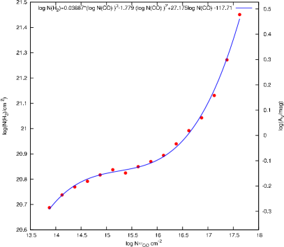
Figure 14.— The average $N({\rm H}_{2})$ and $A_{\rm V}$ as a function of $N({\rm CO})$ in Mask1. $N({\rm H}_{2})$ is estimated from $A_{\rm V}$ assuming $N({\rm H}_{2})/A_{\mathrm{V}}=9.4\times 10^{20}{\rm cm}^{-2}\,{\rm mag}^{-1}$ (Bohlin et al., 1978).

We also include in Figure 13 the fit to the observations from Sheffer et al. (2008) toward diffuse molecular Galactic lines–of–sight for log($N({\rm H}_{2}))\geq 20.4$. The fit seems to agree with the portion our data points that agree fairly well with the model having $\chi=1.0$. Since Sheffer et al. (2008) observed diffuse lines-of-sight, this suggests that a large fraction of the material in the Taurus molecular cloud is shielded against the effect of the FUV illumination. This is supported by infrared observations in Taurus by Flagey et al. (2009) that suggest that the strength of the FUV radiation field is between $\chi=0.3$ and 0.8.

Sheffer et al. (2008, see also ) showed empirical and theoretical evidence that the scatter in the $A_{\rm V}-N({\rm CO})$ relation is due to variations of the ratio between the total H volume density ($n^{\rm total}_{\rm H}=n_{\rm H}+2n_{\rm H_{2}}$) and the strength of the FUV radiation field. The larger the volume density or the weaker the strength of the FUV field the larger the abundance of CO relative to H₂. Note that the scatter in the observations from Sheffer et al. (2008) is much smaller than that shown in Figure 13. This indicates that we are tracing a wider range of physical conditions of the gas. The excitation temperature of the gas observed by Sheffer et al. (2008) does not show a large variation from $T_{\rm ex}$=5 K while we observe values between 4 and 15 K.

In Figure 13 we see that some regions can have large [¹²CO]/[H₂] abundance ratios but still have very small column densities ($A_{\rm V}=0.1-0.5$ mag). This can be understood in terms of a medium which is made of an ensemble of spatially unresolved dense clumps embedded in a low density interclump medium (Bensch, 2006). In this scenario, the contribution to the total column density from dense clumps dominates over that from the tenuous inter–clump medium. Therefore the total column density is proportional to the number of clumps along the line–of–sight. A low number of clumps along a line–of–sight would give low column densities while in the interior of these dense clumps CO is well shielded against FUV photons and therefore it can reach the asymptotic value of the [CO]/[H₂] ratio characteristic of dark clouds.

4. Discussion

4.1. The mass of the Taurus Molecular Cloud

In this section we estimate the mass of the Taurus Molecular Cloud using the $N({\rm CO})$ and $A_{\rm V}$ maps. The masses derived for Mask 0, 1, and 2 are listed in Table 3. To derive the H₂ mass from $N({\rm CO})$ we need to apply an appropriate [CO]/[H₂] relative abundance for each mask. The simplest case is Mask 2 where we used the asymptotic ¹²CO abundance of 1.1$\times$10^-4 (see Section 3.1). We corrected for saturation including temperature gradients and for depletion in the mass calculation from $N({\rm CO})$. These corrections amount to $\sim$319 M_⊙ (4 M_⊙ from the saturation correction and 315 M_⊙ from the addition of the column density of CO–ices). For Mask 1 and 0, we use the fit to the relation between $N({\rm H}_{2})$ and $N({\rm CO})$ shown in Figure 14. As we can see in Table 3, the masses derived from $A_{\rm V}$ and $N({\rm CO})$ are very similar. This confirms that $N({\rm CO})$ is a good tracer of the bulk of the molecular gas mass if variations of the [CO]/[H₂] abundance ratio are considered.

Most of the mass derived from $A_{\rm V}$ in Taurus is in Mask 2 ($\sim$49%). But a significant fraction of the total mass lies in Mask 1 ($\sim$28%) and Mask 0 ($\sim$23%). This implies that mass estimates that only consider regions where ¹³CO is detected underestimate the total mass of the molecular gas by a factor of $\sim$2.

We also estimate the masses of high–column density regions considered by Goldsmith et al. (2008) that were previously defined by Onishi et al. (1996). In Table 4 we list the masses derived from the visual extinction as well as from $N({\rm CO})$. Again, both methods give very similar masses. These regions together represent 43% of the total mass in our map of Taurus, 32% of the area, and 46% of the ¹²CO luminosity. This suggest that the mass and ¹²CO luminosity are uniformly spread over the area of our Taurus map.

A commonly used method to derive the mass of molecular clouds when only ¹²CO is available is the use of the empirically derived CO–to–H₂ conversion factor ($X_{\rm CO}\equiv N({\rm H}_{2})/I_{\rm CO}\simeq M_{{\rm H}_{2}}/L_{\rm CO}$ ). Observations of $\gamma$-rays indicate that this factor is 1.74$\times 10^{20}$ cm^-2(K km s^-1 pc^-2)^-1 or $M({\rm M}_{\odot}$)=3.7$L_{\rm CO}$ (K Km s^-1 pc²) in our Galaxy (Grenier et al., 2005). To estimate $X_{\rm CO}$ in Mask 2, 1, and 0 we calculate the ¹²CO luminosity ($L_{\rm CO}$) in these regions and compare them with the mass derived from $A_{\rm V}$. We also calculate $X_{\rm CO}$ from the average ratio of $N({\rm H}_{2})$ (derived from $A_{\rm V}$ ) to the CO integrated intensity $I_{\rm CO}$ for all pixels in Mask 1 and 2. For Mask 0, we used the ratio of the average $N({\rm H}_{2})$ (derived from $A_{\rm V}$ ) to the average CO integrated intensity obtaining after combining all pixels in this mask region. The resulting values are shown in Table 3. The table shows that the difference in $X_{\rm CO}$ between Mask 2 and Mask 1 is small considering that the [CO]/[H₂] relative abundance between these regions can differ by up to two orders of magnitude. The derived values are close to that found in our Galaxy using $\gamma$-ray observations. For Mask 0, however, $X_{\rm CO}$ is about an order of magnitude larger than in Mask 1 and 2.

Finally we derive the surface density of Taurus by comparing the total H₂ mass derived from $A_{\rm V}$ (15015 M_⊙) and the total area of the cloud (388 pc²). Again, we assumed that in Mask 0 the CO–emitting region occupies 26% of the area. The resulting surface density is $\sim$39 M_⊙ pc^-2 which is very similar to the median value of 42 M_⊙ pc^-2 derived from a large sample of galactic molecular clouds by Heyer et al. (2009).

Table 3Properties of Different Mask Regions in Taurus

Region	# of Pixelsa	Mass from	Mass from	Area	$[{\rm CO}]/[{\rm H}_{2}]$	$L_{\rm CO}$	$X^{b}_{\rm CO}=N({\rm H}_{2})$/$I_{\rm CO}$	$X^{c}_{\rm CO}=M/L_{\rm CO}$
		13CO and 12CO	$A_{\rm V}$
		[$M_{\odot}$]	[$M_{\odot}$]	[pc2]		[K km s-1 pc2]	[cm-2/(K km s-1)]	[$M_{\odot}$/(K km s-1 pc2)]
Mask 0	52338	3267	3454	63d	1.2$\times 10^{-6}$	130	1.2$\times 10^{21}$	26
Mask 1	40101	3942	4237	185	variable	1369	1.6$\times 10^{20}$	3.1
Mask 2	30410	7964	7412	140	1.1$\times 10^{-4}$	1746	2.0$\times 10^{20}$	4.2
Total	122849	15073	15103	388		3245	2.3$\times 10^{20}$	4.6

4.2. Column density probability density function

Table 4Mass of Different High Column Density Regions in Taurus

Region	# of Pixels	Mass from	Mass from	Area	$L_{\rm CO}$
		13CO and 12CO	$A_{\rm V}$
		[$M_{\odot}$]	[$M_{\odot}$]	[pc2]	[K km s-1 pc2]
L1495	7523	1836	1545	35	461
B213	2880	723	640	13	155
L1521	4026	1084	1013	19	236
HCL2	3633	1303	1333	17	221
L1498	1050	213	170	5	39
L1506	1478	262	278	7	68
B18	3097	828	854	14	195
L1536	3230	474	579	15	134
Total	26917	6723	6412	125	1509

Figure 15.— Probability density function of the visual extinction in the Taurus molecular cloud. The solid line corresponds to a Gaussian fit to the distribution of the natural logarithms of $A_{\rm V}/\langle A_{\rm V}\rangle$. This fit considers only visual extinctions that are lower than 4.4 mag, as the distribution deviates clearly from a Gaussian for larger visual extinctions. (see text).

Numerical simulations have shown that the probability density function (PDF) of volume densities in molecular clouds can be fitted by a log-normal distribution. This distribution is found in simulations with or without magnetic fields when self-gravity is not important (Ostriker et al., 2001; Nordlund & Padoan, 1999; Li et al., 2004; Klessen, 2000). A log-normal distribution arises as the gas is subject to a succession of independent compressions or rarefactions that produce multiplicative variations of the volume density (Passot & Vázquez-Semadeni, 1998; Vázquez-Semadeni & García, 2001). This effect is therefore additive for the logarithm of the volume density. A log-normal function can also describe the distribution of column densities in a molecular cloud if compressions or rarefactions along the line of sight are independent (Ostriker et al., 2001; Vázquez-Semadeni & García, 2001). Note that log–normal distributions are not an exclusive result of supersonic turbulence as they are also seen in simulations with the presence of self–gravity and/or strong magnetic fields but without strong turbulence (Tassis et al., 2010).

Deviations from a log-normal in the form of tails at high or low densities are expected if the equation of state deviates from being isothermal (Passot & Vázquez-Semadeni, 1998; Scalo et al., 1998). This, however, also occurs in simulations with an isothermal equation of state due to the effects of self-gravity (Tassis et al., 2010).

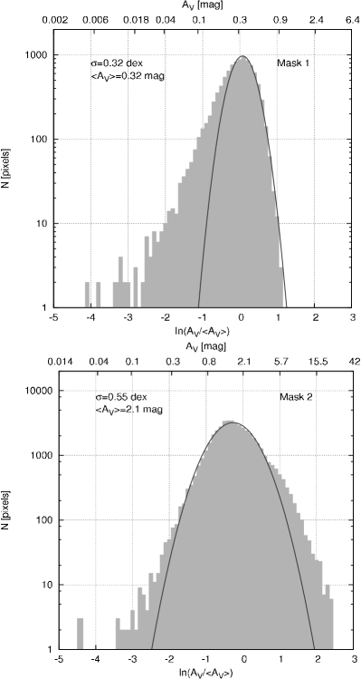
Figure 16.— Probability density function of the visual extinction for Mask 1 (upper panel) and Mask 2 (lower panel) in the Taurus molecular cloud. The solid line corresponds to a Gaussian fit to the distribution of the natural logarithm of $A_{\rm V}/\langle A_{\rm V}\rangle$. The fit for Mask1 considers only visual extinctions that are larger than 0.24 mag, while the fit for Mask 2 includes only visual extinctions that are less than 4.4 mag (see text).

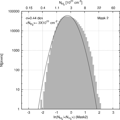
Figure 17.— Probability density function of the H₂ column density derived from $N({\rm CO})$ in Mask 2 with an angular resolution of 47^′′ (0.03 pc at the distance of Taurus, 140 pc). The solid line corresponds to a Gaussian fit to the distribution of the natural logarithm of $N({\rm H}_{2})/\langle N({\rm H}_{2})\rangle$. The fit considers H₂ column densities that are lower than 4$\times 10^{21}$ cm^-2 (or $\sim$4 mag).

In Figure 15 we show the histogram of the natural logarithm of $A_{\rm V}$ in the Taurus molecular cloud normalized by its mean value (1.9 mag). Defining $x\equiv N/\langle N\rangle$, where $N$ is the column density (either $A_{\rm V}$ or $N({\rm H}_{2})$ ), we fit a function of the form

$$f({\ln}x)=N_{\rm pixels}\exp\left[-\frac{({\ln}(x)-\mu)^{2}}{2\sigma^{2}}\right],$$ (29)

where $\mu$ and $\sigma^{2}$ are the mean and variance of $\ln(x)$. The mean of the logarithm of the normalized column density is related to the dispersion $\sigma$ by $\mu=-\sigma^{2}/2$. In all Gaussian fits, we consider $\sqrt{N}$ counting errors in each bin.

The distribution of column densities derived from the visual extinction shows tails at large and small $A_{\rm V}$. The large–$A_{\rm V}$ tail starts to be noticeable at visual extinctions larger than $\sim$4.4 mag. The low–$A_{\rm V}$ tail starts to be noticeable at visual extinctions smaller than $\sim$0.26 mag, which is similar to the uncertainty in the determination of visual extinction (0.29 mag), and therefore it is not possible to determine whether it has a physical origin or it is an effect of noise. The distribution is well fitted by a log–normal for $A_{\rm V}$ smaller than 4.4 mag. We searched in our extinction map for isolated regions with peak $A_{\rm V}\gtrsim 4.4$ mag. We find 57 regions that satisfy this requirement. For each region, we counted the number of pixels that have $A_{\rm V}\gtrsim 4.4$ mag and from that calculated their area, $A$. We then determined their size using $L=2\sqrt{(A/\pi)}$. The average value for all such regions is 0.41 pc. This value is similar to the Jeans length, which for $T_{\rm kin}$=10 K and $n({\rm H}_{2})=10^{3}$ cm^-3 is about 0.4 pc. This agreement suggests that the high–$A_{\rm V}$ tail might be a result of self–gravity acting in dense regions. Kainulainen et al. (2009) studied the column density distribution of 23 molecular cloud complexes (including the Taurus molecular cloud) finding tails at both large and small visual extinctions.

Kainulainen et al. (2009) found that high–$A_{\rm V}$ tails are only present in active star–forming molecular clouds while quiescent clouds are well fitted by a log–normal. We test whether this result applies to regions within Taurus in Figure 16 where we show the visual extinction PDF for the Mask 1 and 2 regions. Mask 1 includes lines–of–sights that are likely of lower volume density than regions in Mask 2, and in which there is little star formation. This is illustrated in Figure 1 where we show the distribution of the Mask regions defined in our map overlaid by the compilation of stellar members of Taurus by Luhman et al. (2006). Most of the embedded sources in Taurus are located in Mask 2. Note that the normalization of $A_{\rm V}$ is different in the two mask regions. The average value of $A_{\rm V}$ in Mask 1 is 0.32 mag and in Mask 2 is 2.1 mag. In Mask 1 we see a tail for low–$A_{\rm V}$ starting at about 0.2 mag. Again, this visual extinction is close to the uncertainty in the determination of $A_{\rm V}$. For larger visual extinctions the PDF appears to be well fitted by a log–normal distribution. In case of the visual extinction PDF in Mask 2, we again see the tail at large $A_{\rm V}$ starting at about 4.4 mag. For lower values of $A_{\rm V}$ the distribution is well represented by a log–normal.

We can use our CO map of Taurus at its original resolution (47^′′ which corresponds to 0.03 pc at the distance of Taurus, 140 pc) to study the column density PDF at higher resolution than the 200^′′ $A_{\rm V}$ map (Figure 17). We estimate $N({\rm H}_{2})$ from our CO column density map in Mask 2 by applying a constant [CO]/[H₂] abundance ratio of 1.1$\times$10^-4 (Section 3.1). The average H₂ column density in Mask 2 is $3\times 10^{21}$ cm^-2. We do not consider Mask 1 because of the large scatter found in the [CO]/[H₂] abundance ratio (Section 3.2). In the figure we see that the distribution is not well fitted by a log–normal. As for $A_{\rm V}$, the PDF also shows a tail for large column densities that starts to be noticeable at about $4\times 10^{21}$ cm^-2 (or $A_{\rm V}\simeq 4$ mag). Therefore, the high–column density excess seems to be independent of the spatial scale at which column densities are sampled. We repeated the procedure described above to search for isolated cores in our map with $N({\rm H}_{2})>4\times 10^{21}$ cm^-2 and obtained an average size for cores of 0.5 pc, which is consistent to that obtained in our $A_{\rm V}$ map . Note that at this resolution we are not able to account for effects of temperature gradients and of CO depletion along the line of sight, as this requires knowledge of $A_{\rm V}$ at the same resolution. We therefore underestimate the number of pixels in the H₂ column density PDF for $N({\rm H}_{2})\gtrsim 1\times 10^{22}$ cm^-2 while we overestimate them for $N({\rm H}_{2})\lesssim 1\times 10^{22}$ cm^-2. But the number of pixels ($\sim$7000) affected by those effects represent only 9% of the number of pixels ($\sim$81000) that are in excess relative to the log–normal fit between $3\times 10^{21}$ and $1\times 10^{22}$ cm^-2, and therefore the presence of a tail at large–$N({\rm H}_{2})$ is not affected. Note that this also affected our ability to identify isolated regions in the $N({\rm H}_{2})$ map. We were able to identify only 40 cores compared with the 57 found in the $A_{\rm V}$ map.

In summary, we find that the distribution of column densities in Taurus can be fitted by a log–normal distribution but shows tails at low and high–column densities. The tail at low–column density may be due to noise and thus needs to be confirmed with more sensitive maps. We find that the tail at large column densities is only present in the region where most of the star formation is taking place in Taurus (Mask 2) and is absent in more quiescent regions (Mask 1). The same trend has been found in a larger sample of clouds by Kainulainen et al. (2009). Here we suggest that the distinction between star-forming and non star-forming regions can be found even within a single molecular cloud complex. The presence of tails in the PDF in Taurus appears to be independent of angular resolution and is noticeable for length scales smaller than 0.41 pc.

5. Conclusions

In this paper we have compared column densities derived from the large scale ¹²CO and ¹³CO maps of the Taurus molecular cloud presented by Narayanan et al. 2008 (see also Goldsmith et al. 2008) with a dust extinction map of the same region. This work can be summarized as follows,

• We have improved the derivation of the CO column density compared to that derived by Goldsmith et al. (2008) by using an updated value of the spontaneous decay rate and using exact numerical rather than approximate analytical calculation of the partition function. We also have used data that has been corrected for error beam pick–up using the method presented by Bensch et al. (2001).

• We find that in the Taurus molecular cloud the column density and visual extinction are linearly correlated for $A_{\rm V}$ up to 10 mag in the region associated with the B213–L1495 filament. In the rest of Taurus, this linear relation is flattened for $A_{\rm V}\gtrsim 4$ mag. A linear fit to data points for $A_{\rm V}<10$ mag and $N({\rm CO})>10^{17}$ cm^-2 results in an abundance of CO relative to H₂ equal to 1.1$\times$10^-4.

• For visual extinctions larger than $\sim$4 mag the CO column density is affected by saturation effects and freezeout of CO molecules onto dust grains. We find that the former effect is enhanced due to the presence of edge–to–center temperature gradients in molecular clouds. We used the RATRAN radiative transfer code to derive a correction for this effect.

• We combined the column density of CO in ice form derived from observations towards embedded and field stars in Taurus by Whittet et al. (2007) with the saturation–corrected gas–phase $N({\rm CO})$ to derive the total CO column density (gas–phase+ices). This quantity is linearly correlated with $A_{\rm V}$ up to the maximum extinction in our data $\sim$23 mag.

• We find that the gas–phase CO column density is reduced by up to a factor of $\sim$2 in high–extinction regions due to depletion in the Taurus molecular cloud.

• We fit an analytical column density profile to 13 cores in Taurus. The mean value and standard deviation of the central volume density are ($1.4\pm 0.4$)$\times 10^{4}$ cm^-3. We use the derived volume density profile and the amount of depletion observed in each core to derive an upper limit to the CO depletion age with a mean value and standard deviation of $(4.2\pm 2.4)\times 10^{5}$ years. We find little variation of this age among the different regions within Taurus.

• For visual extinctions lower than 3 mag we find that $N({\rm CO})$ is reduced by up to two orders of magnitude due to the competition between CO formation and destruction processes. There is a large scatter in the $A_{\rm V}$ –$N({\rm CO})$ relation that is suggestive of different FUV radiation fields characterizing the gas along different lines–of–sight.

• The mass of the Taurus molecular cloud is about 1.5$\times 10^{4}\,$M_⊙. Of this, $\sim$49% is contained in pixels where both ¹²CO and ¹³CO are detected (Mask 2), $\sim$28% where ¹²CO is detected but ¹³CO is not (Mask 1), and $\sim$23% where neither ¹²CO nor ¹³CO are detected (Mask 0).

• We find that the masses derived from CO and $A_{\rm V}$ are in good agreement. For Mask 2 and Mask 0 we used a [CO]/[H₂] relative abundance of 1.1$\times$10^-4 and 1.2$\times 10^{-6}$, respectively. For Mask 1, we used a variable [CO]/[H₂] relative abundance taken from a fit to the average relation between $A_{\rm V}$ and $N({\rm CO})$ in this region, with $-6.7<\log([{\rm CO}]/[\rm H_{2}])\leq-3.9$.

• We also compared the mass derived from $A_{\rm V}$ with the ¹²CO $J=1\to 0$ luminosity for the regions derived above. For Mask 1 and 2 these two quantities are related with a CO–to–H₂ conversion factor of about 2.1$\times 10^{20}$cm^-2 (K km s^-1 )^-1. The derived CO–to–H₂ conversion factor is in agreement with that found in our Galaxy using $\gamma$–ray observations. In Mask 0, however, we find a larger the conversion factor of 1.2$\times 10^{21}$cm^-2 (K km s^-1 )^-1.

• We studied the distribution of column densities in Taurus. We find that the distribution resembles a log–normal but shows tails at large and low column densities. The length scale at which the high–column density tail starts to be noticeable is about 0.4 pc, which is similar to the Jeans length for a $T$=10 K and $n_{{\rm H}_{2}}=10^{3}$ cm^-3 gas, suggesting that self–gravity is responsible for its presence. The high–column density tail is only present in regions associated with star formation, while the more quiescent positions in Taurus do not show this feature. This tail is independent of the resolution of the observations.
  

Appendix A Error Beam Correction

The FCRAO 14m telescope is sensitive not only to emission that couples to the main beam (with efficiency $\eta_{\rm mb}$ = 0.45 at 115 GHz and $\eta_{\rm mb}$ = 0.48 at 110 GHz) but also to emission distributed on scales comparable to the error beam (30^′). For emission extended over such large-scale, the coupling factor (including the main beam contribution) is the forward spillover and scattering efficiency, $\eta_{\rm fss}$ = 0.7, at both frequencies. The error beam pickup, also known as “stray radiation”, can complicate the accurate calibration of the measured intensities: a straightforward scaling of the data by 1/$\eta_{\rm mb}$ can significantly overestimate the true intensity in regions where emission is present on large angular scales. Given the wide range of angular sizes of the structures in Taurus, it is clear in general that neither $\eta_{\rm mb}$ nor $\eta_{\rm fss}$ will give optimum results.

To accurately scale the FCRAO data, it is essential to remove the error beam component before scaling the intensities to the main beam scale. Methods for correcting millimeter-wave data for error beam pickup have been discussed by Bensch et al. (2001), who introduce the “corrected main beam temperature scale” ($T_{\rm mb,c}$) with which optimum calibration accuracy is achieved by scaling the data by 1/$\eta_{\rm mb}$ after removal of radiation detected by the error beam.

To remove the error beam component we use the second of the methods described in Bensch et al. (2001). The error beam component is removed in Fourier space directly from the FCRAO data, and the intensities are converted to the $T_{\rm mb,c}$ scale, by the following method:

• The Fourier transform of the antenna temperature is taken: $\tilde{T}_{\rm A}^{*}$ = $FT(T_{\rm A}^{*})$

• The following correction is applied to each velocity slice in the cube:

  $$\tilde{T}_{\rm mb,c}=\tilde{T}_{\rm A}^{*}(\eta_{\rm mb}+\eta_{\rm eb}\exp(\frac{-\pi^{2}(\theta_{\rm eb}^{2}-\theta_{\rm mb}^{2})(k_{x}^{2}+k_{y}^{2})}{4\ln(2)}))^{-1}$$

  where $\theta_{\rm eb}$ is the FWHM of the error beam, $\theta_{\rm mb}$ is the FWHM of the main beam, $\eta_{\rm eb}=\eta_{\rm fss}-\eta_{\rm mb}$, and $k_{x}$, $k_{y}$ are the wavenumbers along the $x$, $y$ (RA, decl.) directions respectively.

• The inverse Fourier transform is performed, with only the real part of the result being retained: $T_{\rm mb,c}$ = $Re~{}(IFT(\tilde{T}_{\rm mb,c}))$. The imaginary part is consistent with round–off errors.

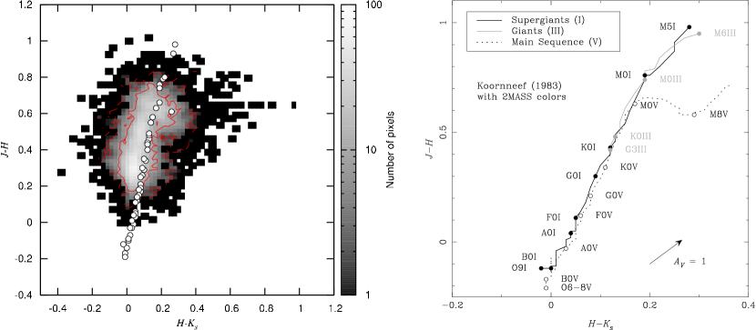
Figure 18.— (left) Color $(H-K_{s})$ versus $(J-H)$ for stars observed in the control field. (right) Intrinsic $J-H$ and $H-K_{s}$ colors of Main Sequence, Giant, and Supergiant stars (taken from Koornneef 1983). These stars are indicated by circles in the left panel.

At low spatial frequencies, the correction factor is $\sim$ 1/$\eta_{\rm fss}$ while at high spatial frequencies, the correction factor is $\sim$ 1/$\eta_{\rm mb}$. The effective correction factor at any point is determined therefore by the spatial structure of the emission in the vicinity of that point. More detailed information and quantitative analysis of the above procedure can be found in Brunt et al (2010, in prep) and Mottram & Brunt (2010, in prep). For typical applications, a naive scaling by 1/$\eta_{\rm mb}$ overestimates the true intensities, as inferred from comparison to CfA survey data (Dame et al., 2001), by around 25–30%. For reference, an overestimation of $\sim$ 50% would be applicable if $\eta_{\rm fss}$ were appropriate everywhere. The spatially variable correction factor afforded by the method used here therefore offers a higher fidelity calibration of the data.

Appendix B The Extinction Map

We have used the 2MASS point source catalog to create an near–infrared extinction map of Taurus. This was done using an implementation of NICER (Lombardi & Alves, 2001) from Chapman (2007). The 2MASS catalog we used has 1039735 ($\sim$1 million) stars over an area between RA=04:03:51.6 and 05:05:56.6 and decl.=+19:24:14.4 and +30:50:24 (J2000). We use the compilation by Luhman et al. (2006) to remove 156 stars that are known to be members of Taurus. The map generated has an angular resolution of 200^′′ and is Nyquist sampled with a pixel spacing of 100^′′, corresponding to 0.07 pc at a distance of 140 pc. The resolution of the map was determined by that of the H i map used to correct the data for the contribution of H i to the total extinction (see below). The final extinction map is shown in Figure 4.

We constructed extinction maps in nearby regions around Taurus with the goal of finding a field that does not show significant extinction, so it can be used as a control field to estimate the intrinsic $(J-H)$ and $(H-K_{s})$ stellar colors. We selected a region corresponding to a $2^{\circ}\times 2^{\circ}$ box centered at RA=03:50:44.7 and decl.=+27:46:54.1 (J2000). The mean ($\pm$ weighted standard deviation) values for stars in this box are 0.454$\pm$0.157 mag for $(J-H)$ and 0.114$\pm$0.074 mag for $(H-K_{s})$. We also computed the covariance matrix for the $(J-H)$ and $(H-K_{s})$ colors. The on-axis elements of this matrix are $\sigma_{J-H}^{2}$ and $\sigma_{H-K_{s}}^{2}$, the dispersions of the $(J-H)$ and $(H-K_{s})$ colors in the control field, while the two off–axis elements are identical to each other, with a value of 0.006. In Figure 18 we show the color $(H-K_{s})$ versus $(J-H)$ of stars in the control field. We also show the intrinsic color of Main Sequence, Giant, and Supergiant stars. Apart from the scatter due to photometric errors, there is large scatter in the intrinsic colors due to different stellar types in the control field. The mean values, weighted standard deviation and off–axis covariance matrix are input to the NICER routine and with them we correct for the different sources of scatter of the intrinsic colors in the control field. Note that Padoan et al. (2002) used an intrinsic $(H-K_{s})$ color of 0.13 mag in their extinction map of Taurus. The difference relative to that in our control field is thus seen to be small.

We transformed the $(J-H)$ and $(H-K_{s})$ colors to $A_{\rm V}$ using an extinction curve from Weingartner & Draine (2001) with a ratio of selective to total extinction $R_{\rm V}$=3.1. Note that this $R_{\rm V}$ is derived towards diffuse regions ($A_{\rm V}\leq$ 1.5 mag). At larger volume densities the value of $R_{V}$ is expected to increase up to 4.5 at the center of dense cores due to grain growth by accretion and coagulation (Whittet et al., 2001). Considering that a given line–of–sight might intersect both dense and diffuse regions, Whittet et al. (2001) estimated an effective $R_{\rm V}$ that increases up to $\sim 4.0$ for $A_{\rm V}$ $\simeq 10$ mag. For such a value of $A_{\rm V}$ we expect that for a given total hydrogen column density, the visual extinction increases by about 20% due to enhanced scattering as the grain sizes increases (Draine, 2003).

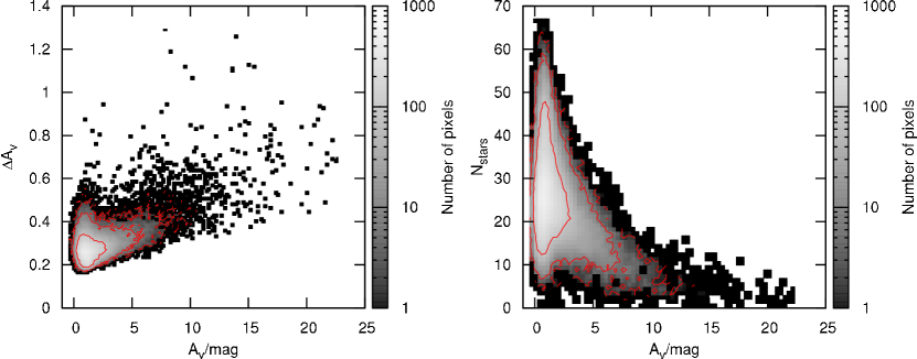
Figure 19.— The formal error per pixel (left) and the number of stars per pixel (right) as a function of the visual extinction estimated in the Taurus molecular cloud.

Figure 19 shows the relation between the estimated visual extinction in the Taurus molecular cloud and the formal error per pixel (i.e. error propagation from the error in the estimation of $A_{\rm V}$ for each star) and the number of stars per pixel. The errors in $A_{\rm V}$ range from $\sim$0.2 mag at low extinctions to $\sim$1.3 mag at large visual extinctions. The average error is 0.29 mag while the average number of stars per pixel is 28. As expected, the number of stars per pixel decreases as the extinction increases.

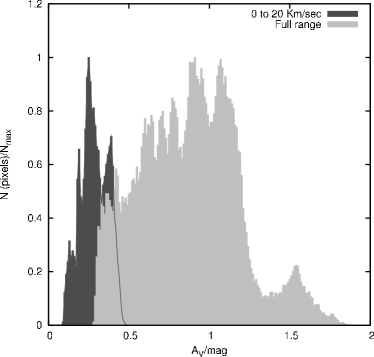
Figure 20.— Histogram of the visual extinction in Taurus associated with H i for the full range of 21 cm velocities (light gray) and for the velocity range between 0 and 20 km s^-1 (dark gray). The histogram has been determined for the region where both ¹²CO and ¹³CO are detected.

There is a large filamentary Hi structure, extending away from the Galactic plane, which coincides with the eastern part of Taurus. Based on distances of molecular clouds at the end of the filament, we assume that this filament lies between the Taurus background stars and the Earth. Dust in the filament will thus contribute to the total extinction measured. We estimate the contribution to the visual extinction from dust associated with H i using the Arecibo map from Marco Krčo (PhD Thesis, Cornell University, in preparation). In Figure 20 we show a histogram of the visual extinction associated with positions in the H i map where both ¹²CO and ¹³CO are detected in our Taurus map. We show the extinction for the full range of velocities and for the range between 0 to 20 km s^-1 (similar to the velocity range at which CO emission is observed). We correct the $A_{\rm V}$ map by extinction associated with neutral hydrogen in the latter range (see below). The average correction is $\sim$0.3 mag.

In order to see whether some H i velocity components are foreground to the 2MASS stars, we examine a field with complex H i velocity structure. We choose a region northwest of the Taurus molecular cloud that shows small visual extinction (RA = 04:57:25.472 and decl. = 29:07:0.81). Figure 21a shows a histogram of the visual extinction without correction, corrected for H i over the entire velocity range, and corrected for H i over the 0 to 20 km s^-1 range. We also show in Figure 21b the average H i spectrum in the selected field. The negative velocity components produce significant excess reddening associated with H i that is inconsistent with the extinction determined from 2MASS stars. We therefore conclude that H i components with negative velocities are background to the 2MASS stars. This confirms the correctness of excluding negative velocities for determining the H i-associated extinction correction for Taurus. The exact velocity range used is a source of uncertainty of a few tenths of a magnitude in the extinction.

We finally note that the widespread H i emission is also present in the control field. The control field is contaminated by $\sim$0.12 mag of visual extinction associated with H i. This contribution produces a small overestimation of the intrinsic colors in the control field. Therefore, since we determine visual extinctions based on the difference between the observed stellar colors in Taurus and those averaged over the control field, we have added 0.12 mag to our final $A_{\rm V}$ map of Taurus.

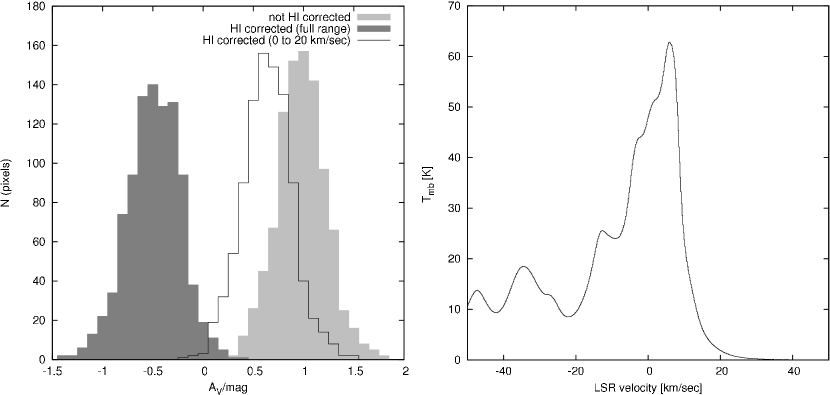
Figure 21.— (left) Histogram of the visual extinction calculated in a field with complex velocity structure (see text) with and without correction for extinction associated with H i. (right) The H i spectrum averaged over the this field.

Appendix C Correction for Temperature Gradients along the Line–of–Sight

In order to assess the impact of core-to-edge temperature gradients in the estimation of $N({\rm CO})$, we use the radiative transfer code RATRAN (Hogerheijde & van der Tak, 2000). With RATRAN we calculate ¹²CO and ¹³CO line profiles and integrated intensities from a model cloud and use them to estimate $N({\rm CO})$, following our analytic procedure (Section 2), which we then compare with that of the original model cloud.

The model is a spherical cloud with a truncated power-law density profile. We adopt a density profile $n(r)$=$n_{\mathrm{s}}(r/r_{\mathrm{c}})^{-\alpha}$ for 0.3$r_{\mathrm{c}}$ $\leq$ $r\leq r_{\mathrm{c}}$, and constant density, $n(r)=n_{s}$(0.3)^-α in the central portion of the cloud ($r<0.3r_{\mathrm{c}}$). Here, $r_{\mathrm{c}}$ is the cloud radius and $n_{\mathrm{s}}$ the density at the cloud surface. In our models we use a power–law exponent of $\alpha$ = 1.96 for the density profile, a density at the cloud surface of 2$\times$10⁴ cm^-3, and a cloud radius of 5$\times$10¹⁶ cm (0.015 pc at a distance of 140 pc). The values of the density at the cloud surface and the power–law exponent are taken from the fit to the extinction profile of the prestellar core B68 (Alves et al., 2001). We adopt a FWHM line-width in the model of $\Delta v$=1.33 km s^-1, in order to have line widths that are consistent with those in pixels having $A_{\rm V}>$ 10 mag (Figure 22). We use the ¹³CO and ¹²CO emission resulting from the radiative transfer calculations to derive, using Equation (17), the CO column density ($N({\rm CO})_{\rm emission}$) that will be compared with that of the model cloud ($N({\rm CO})_{\rm model}$). We trace CO column densities between 3$\times 10^{16}$ cm^-2 and 1$\times 10^{18}$ cm^-2.

We consider the case of isothermal clouds and of clouds with temperature gradients. Temperature gradients can be produced, for example, when clouds are externally illuminated by the interstellar radiation field (e.g. Evans et al., 2001). We adopt a temperature profile given by

$$T(r)=(T_{\rm s}-T_{\rm c})\left(\frac{r}{r_{\rm c}}\right)^{2}+T_{\rm c},$$ (C1)

where $T_{\rm c}$ and $T_{\rm s}$ are the temperature at the cloud center and surface, respectively.

We run isothermal cloud models with kinetic temperatures of 8, 9, 10,12, and 15 K. In the case of clouds with temperature gradients we consider the same range of temperatures for the cloud surface and $T_{\rm c}=8$ K for the cloud center. We choose this value because the balance between the dominant heating and cooling mechanisms in dense and shielded regions, namely cosmic-ray heating and cooling by gas-grain collisions, typically results in this range of temperatures (Goldsmith, 2001). The selected range of temperatures match the observed range of excitation temperatures for $A_{\rm V}>10$ mag (Figure 22).

Figure 22.— Pixel-by-pixel comparison between the visual extinction ($A_{\rm V}$) and the ¹²CO-derived excitation temperature (left ) and ¹³CO FWHM line–width (right).

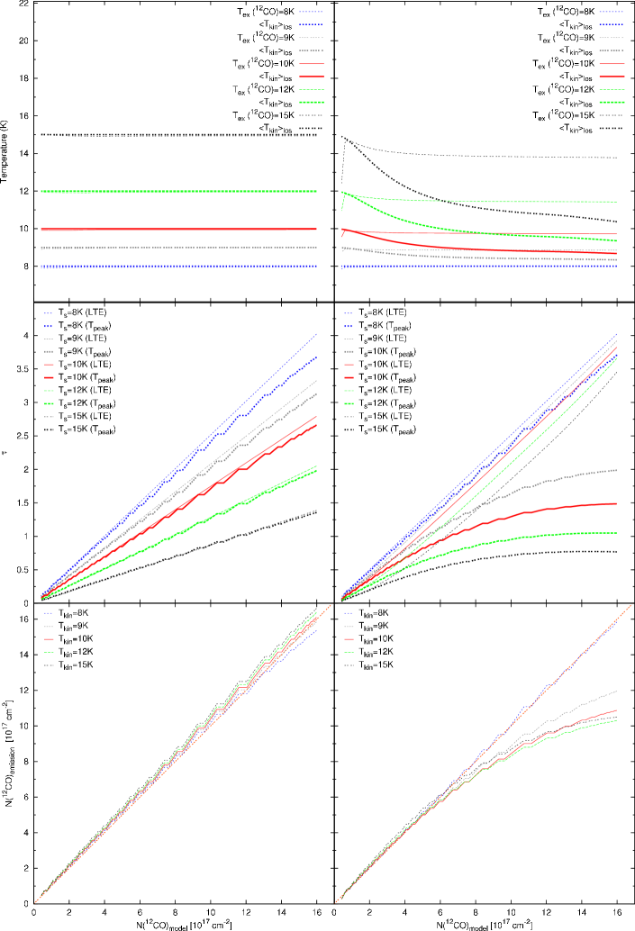
Figure 23.— (upper row) Excitation temperature derived from the ¹²CO emission as function of $N({\rm CO})_{\rm model}$ for isothermal cloud models (left ) and models with temperature gradients (right). In both panels we also show the model cloud kinetic temperature averaged along the line of sight, $\langle T_{\rm kin}\rangle_{\rm los}$, as a function of $N({\rm CO})_{\rm model}$. (middle row) The ¹³CO opacity versus $N({\rm CO})_{\rm model}$ for the models shown in the upper row. The opacity was derived using Equation (20). We also show the opacity calculated from the model cloud N(¹³CO) with the assumption of LTE. (lower row) Column density of CO calculated from the ¹²CO and ¹³CO emission using Equation (17) versus the model cloud $N({\rm CO})$. The straight line corresponds to an one–to–one relation.

In the upper rows of Figure 23 we show the excitation temperature derived from the model ¹²CO emission as a function of $N({\rm CO})_{\rm model}$. The left panel corresponds to isothermal clouds and the right panel to clouds with temperature gradients. We also show the line-of-sight (LOS) averaged kinetic temperature as a function of $N({\rm CO})_{\rm model}$. In clouds with temperature gradients, low column densities are on average warmer than larger column densities. For isothermal clouds $T_{\rm ex}$ and the model kinetic temperature are almost identical for all values of $N({\rm CO})_{\rm model}$. In the case of clouds with temperature gradients we see that, although the average LOS kinetic temperature decreases for large CO column densities, the derived excitation temperature shows little variation with $N({\rm CO})_{\rm model}$, tracing only the temperature at the cloud surface. This is a result of ¹²CO becoming optically thick close to the cloud surface and therefore the $T_{\rm ex}$ determined in this manner applies only to this region. In clouds with temperature gradients, using ¹²CO to calculate the excitation temperature overestimates its value for regions with larger column densities, where most of the ¹³CO emission is produced.

We show the ¹³CO opacity (Equation [20]) for both isothermal clouds and clouds with temperature gradients as a function of $N({\rm CO})_{\rm model}$ in the middle panels of Figure 23. We also show opacities calculated from the model cloud ¹³CO column densities assuming LTE ($\tau_{\rm LTE}$). When the cloud kinetic temperature is constant, both opacities show good agreement for all sampled values of $N({\rm CO})_{\rm model}$. In contrast, for clouds with temperature gradients, opacities derived from the model line emission are lower than $\tau_{\rm LTE}$ by up to a factor of $\sim$3. The differences arise due to the overestimation of the excitation temperature in regions with large $N({\rm CO})$, as Equation [20] assumes a constant value of $T_{\rm ex}$.

The relation between $N({\rm CO})_{\rm emission}$ and $N({\rm CO})_{\rm model}$ is shown in the lower panels of Figure 23. Isothermal clouds show almost a one-to-one relation between these two quantities whereas clouds with temperature gradients show that the relation deviates from linear for large $N({\rm CO})_{\rm model}$. This is produced by the underestimation of opacities that affect the correction for this quantity (Equation [15]). The difference between $N({\rm CO})_{\rm emission}$ and the expected CO column density is about 20%.

In the following we use the relation between $N({\rm CO})_{\rm model}$ and $N({\rm CO})_{\rm emission}$ to derive a correction to the observed CO column densities. We notice that the difference between these quantities does not show a strong dependence in the cloud surface temperature. This is because all models have the same temperature at the cloud center. Since the observed excitation temperatures lie between $\sim 9-15$ K for $A_{\rm V}>10$ mag (Figure 23), and the excitation temperature derived from ¹²CO is similar to the kinetic temperature at the cloud surface, we average all models from $T_{\rm s}=9\,$K to 15 K in steps of 1 K to derive a correction function. In Figure 24 we show the difference between the model and derived CO column density ($N({\rm CO})_{\rm diff}=N({\rm CO})_{\rm model}-N({\rm CO})_{\rm emission}$) as a function of the model CO column density. To this relation we fit a polynomial function given by

$$\frac{N({\rm CO})_{\rm diff}}{10^{17}{\rm cm}^{-2}}=0.05N({\rm CO})_{\rm model}^{1.9}-0.25N({\rm CO})_{\rm model}+0.17$$ (C2)

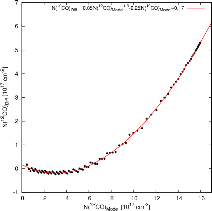
Figure 24.— Difference between the expected $N({\rm CO})_{\rm model}$ and the derived $N({\rm CO})_{\rm emission}$ as a function of the model CO column density. The red line represents a second-order polynomial fit.

To apply this correction we made a rough estimate of the gas–phase CO column density as a function of visual extinction. We use the observations by Frerking et al. (1982) of C¹⁸O and the rarer isotopic species C¹⁷O and ¹³C¹⁸O in the direction of field stars located behind Taurus. We convert the observed column densities into $N({\rm CO})$ assuming [CO]/[C¹⁸O]=557, [C¹⁸O]/[C¹⁷O]=3.6, and [C¹⁸O]/[¹³C¹⁸O]=69 (Wilson, 1999). Due to their low abundances, these species are likely not affected by saturation. Note that, however, they are still sensitive to the determination of the excitation temperature. Frerking et al. (1982) presented column densities as lower limits when ¹²CO is used to determine $T_{\rm ex}$(¹²CO) (average $\sim$10 K) and as upper limits when they used $T_{\rm ex}$(¹²CO)/2 (i.e. $\sim$5 K) as the excitation temperature. The kinetic temperature in dense regions is likely to be in between 5 and 10 K (Goldsmith, 2001) and therefore, assuming that the isotopologues are thermalized, the excitation temperature should also have a value in this range. Thus, we use the average value between upper and lower limits of the CO column density to determine its relation with $A_{\rm V}$. For the visual extinction at the positions observed by Frerking et al. (1982), we use updated values derived by Shenoy et al. (2008) from infrared observations. We note that the visual extinction correspond to a single star while the Frerking et al. (1982) observations are averaged over a 96^′′ beam. We constructed an extinction map of Taurus with 96^′′ resolution and an extinction curve that matches that adopted by Shenoy et al. (2008) in order to compare with their determination of $A_{\rm V}$. We found that the visual extinctions always agree within $\pm 0.4$ mag.

In Figure 25 we show the relation between $N({\rm CO})$ and $A_{\rm V}$ with and without the correction for the effects of temperature gradients along the line–of–sight. For reference we include the values of $N({\rm CO})$ derived from the observations by Frerking et al. (1982). The error bars denote the upper and lower limits to the CO column density mentioned above. Although our determination of the gas–phase $N({\rm CO})$/$A_{\rm V}$ relation is necessarily approximate, the validity of the correction for the effects of temperature gradients along the line–of–sight is confirmed by the good agreement between $A_{\rm V}$ and $N({\rm CO})$ up to $A_{\rm V}\simeq$23 mag after the addition of the column density of CO–ices (Section 3.1.1).

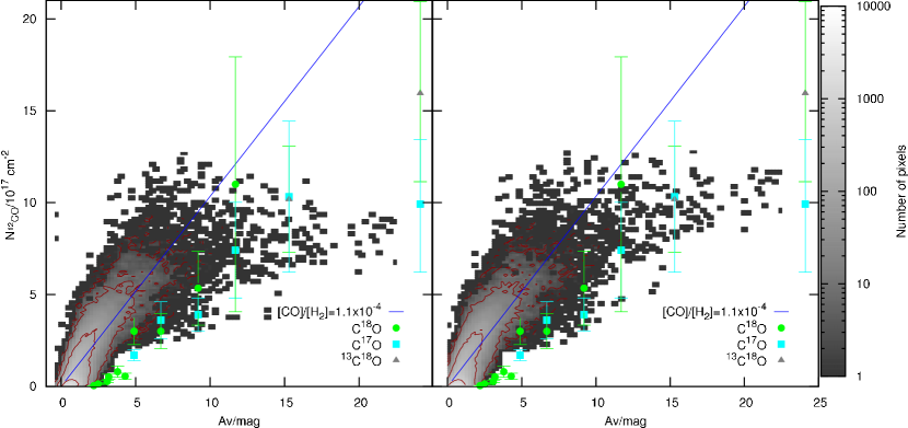
Figure 25.— Pixel-by-pixel comparison between $A_{\rm V}$ and $N({\rm CO})$ as in Figure 6 including the CO column density derived from rare isotopic species observed by Frerking et al. (1982). The left panel shows the CO column densities derived from Equation (17) with the opacity correction from Equation (15), which assumes isothermal gas. The right panel shows $N({\rm CO})$ corrected for saturation including temperature gradients.

References

- Alves et al. (1999) Alves, J., Lada, C. J., & Lada, E. A. 1999, ApJ, 515, 265
- Alves et al. (2001) Alves, J. F., Lada, C. J., & Lada, E. A. 2001, Nature, 409, 159
- Bensch (2006) Bensch, F. 2006, A&A, 448, 1043
- Bensch et al. (2001) Bensch, F., Stutzki, J., & Heithausen, A. 2001, A&A, 365, 285
- Bergin et al. (2002) Bergin, E. A., Alves, J., Huard, T., & Lada, C. J. 2002, ApJ, 570, L101
- Bergin & Langer (1997) Bergin, E. A. & Langer, W. D. 1997, ApJ, 486, 316
- Bergin & Tafalla (2007) Bergin, E. A. & Tafalla, M. 2007, ArXiv e-prints, 705
- Bisschop et al. (2006) Bisschop, S. E., Fraser, H. J., Öberg, K. I., van Dishoeck, E. F., & Schlemmer, S. 2006, A&A, 449, 1297
- Bohlin et al. (1978) Bohlin, R. C., Savage, B. D., & Drake, J. F. 1978, ApJ, 224, 132
- Burgh et al. (2007) Burgh, E. B., France, K., & McCandliss, S. R. 2007, ApJ, 658, 446
- Cambrésy (1999) Cambrésy, L. 1999, A&A, 345, 965
- Caselli et al. (1999) Caselli, P., Walmsley, C. M., Tafalla, M., Dore, L., & Myers, P. C. 1999, ApJ, 523, L165
- Chapman (2007) Chapman, N. L. 2007, PhD thesis, University of Maryland, College Park
- Chiar et al. (1995) Chiar, J. E., Adamson, A. J., Kerr, T. H., & Whittet, D. C. B. 1995, ApJ, 455, 234
- Dame et al. (2001) Dame, T. M., Hartmann, D., & Thaddeus, P. 2001, ApJ, 547, 792
- Dapp & Basu (2009) Dapp, W. B. & Basu, S. 2009, MNRAS, 395, 1092
- Dobashi et al. (2005) Dobashi, K., Uehara, H., Kandori, R., Sakurai, T., Kaiden, M., Umemoto, T., & Sato, F. 2005, PASJ, 57, 1
- Draine (1978) Draine, B. T. 1978, ApJS, 36, 595
- Draine (2003) —. 2003, ARA&A, 41, 241
- Evans et al. (2001) Evans, II, N. J., Rawlings, J. M. C., Shirley, Y. L., & Mundy, L. G. 2001, ApJ, 557, 193
- Federman et al. (1980) Federman, S. R., Glassgold, A. E., Jenkins, E. B., & Shaya, E. J. 1980, ApJ, 242, 545
- Flagey et al. (2009) Flagey, N., Noriega-Crespo, A., Boulanger, F., Carey, S. J., Brooke, T. Y., Falgarone, E., Huard, T. L., McCabe, C. E., Miville-Deschênes, M. A., Padgett, D. L., Paladini, R., & Rebull, L. M. 2009, ApJ, 701, 1450
- Frerking et al. (1982) Frerking, M. A., Langer, W. D., & Wilson, R. W. 1982, ApJ, 262, 590
- Goldsmith (2001) Goldsmith, P. F. 2001, ApJ, 557, 736
- Goldsmith et al. (2008) Goldsmith, P. F., Heyer, M., Narayanan, G., Snell, R., Li, D., & Brunt, C. 2008, ApJ, 680, 428
- Goodman et al. (2009) Goodman, A. A., Pineda, J. E., & Schnee, S. L. 2009, ApJ, 692, 91
- Goorvitch (1994) Goorvitch, D. 1994, ApJS, 95, 535
- Grenier et al. (2005) Grenier, I. A., Casandjian, J.-M., & Terrier, R. 2005, Science, 307, 1292
- Herbst & Klemperer (1973) Herbst, E. & Klemperer, W. 1973, ApJ, 185, 505
- Heyer et al. (2009) Heyer, M., Krawczyk, C., Duval, J., & Jackson, J. M. 2009, ApJ, 699, 1092
- Hogerheijde & van der Tak (2000) Hogerheijde, M. R. & van der Tak, F. F. S. 2000, A&A, 362, 697
- Kainulainen et al. (2009) Kainulainen, J., Beuther, H., Henning, T., & Plume, R. 2009, A&A, 508, L35
- Kainulainen et al. (2006) Kainulainen, J., Lehtinen, K., & Harju, J. 2006, A&A, 447, 597
- King (1962) King, I. 1962, AJ, 67, 471
- Klessen (2000) Klessen, R. S. 2000, ApJ, 535, 869
- Koornneef (1983) Koornneef, J. 1983, A&A, 128, 84
- Kramer et al. (1999) Kramer, C., Alves, J., Lada, C. J., Lada, E. A., Sievers, A., Ungerechts, H., & Walmsley, C. M. 1999, A&A, 342, 257
- Lada et al. (1994) Lada, C. J., Lada, E. A., Clemens, D. P., & Bally, J. 1994, ApJ, 429, 694
- Langer et al. (1989) Langer, W. D., Wilson, R. W., Goldsmith, P. F., & Beichman, C. A. 1989, ApJ, 337, 355
- Li et al. (2004) Li, P. S., Norman, M. L., Mac Low, M., & Heitsch, F. 2004, ApJ, 605, 800
- Liszt (2007) Liszt, H. S. 2007, A&A, 476, 291
- Liszt & Lucas (1998) Liszt, H. S. & Lucas, R. 1998, A&A, 339, 561
- Lombardi & Alves (2001) Lombardi, M. & Alves, J. 2001, A&A, 377, 1023
- Luhman et al. (2006) Luhman, K. L., Whitney, B. A., Meade, M. R., Babler, B. L., Indebetouw, R., Bracker, S., & Churchwell, E. B. 2006, ApJ, 647, 1180
- Maloney & Black (1988) Maloney, P. & Black, J. H. 1988, ApJ, 325, 389
- Narayanan et al. (2008) Narayanan, G., Heyer, M. H., Brunt, C., Goldsmith, P. F., Snell, R., & Li, D. 2008, ApJS, 177, 341
- Nordlund & Padoan (1999) Nordlund, Å. K. & Padoan, P. 1999, in Interstellar Turbulence, ed. J. Franco & A. Carramiñana, 218
- Onishi et al. (1996) Onishi, T., Mizuno, A., Kawamura, A., Ogawa, H., & Fukui, Y. 1996, ApJ, 465, 815
- Ostriker et al. (2001) Ostriker, E. C., Stone, J. M., & Gammie, C. F. 2001, ApJ, 546, 980
- Padoan et al. (2002) Padoan, P., Cambrésy, L., & Langer, W. 2002, ApJ, 580, L57
- Passot & Vázquez-Semadeni (1998) Passot, T. & Vázquez-Semadeni, E. 1998, Phys. Rev. E, 58, 4501
- Penzias (1975) Penzias, A. A. 1975, in Atomic and Molecular Physics and the Interstellar Matter, 373–408
- Roser et al. (2001) Roser, J. E., Vidali, G., Manicò, G., & Pirronello, V. 2001, ApJ, 555, L61
- Ruffle & Herbst (2001) Ruffle, D. P. & Herbst, E. 2001, MNRAS, 324, 1054
- Scalo et al. (1998) Scalo, J., Vazquez-Semadeni, E., Chappell, D., & Passot, T. 1998, ApJ, 504, 835
- Schöier et al. (2005) Schöier, F. L., van der Tak, F. F. S., van Dishoeck, E. F., & Black, J. H. 2005, A&A, 432, 369
- Sheffer et al. (2002) Sheffer, Y., Federman, S. R., & Lambert, D. L. 2002, ApJ, 572, L95
- Sheffer et al. (2008) Sheffer, Y., Rogers, M., Federman, S. R., Abel, N. P., Gredel, R., Lambert, D. L., & Shaw, G. 2008, ApJ, 687, 1075
- Shenoy et al. (2008) Shenoy, S. S., Whittet, D. C. B., Ives, J. A., & Watson, D. M. 2008, ApJS, 176, 457
- Solomon & Klemperer (1972) Solomon, P. M. & Klemperer, W. 1972, ApJ, 178, 389
- Sonnentrucker et al. (2003) Sonnentrucker, P., Friedman, S. D., Welty, D. E., York, D. G., & Snow, T. P. 2003, ApJ, 596, 350
- Tafalla et al. (2002) Tafalla, M., Myers, P. C., Caselli, P., Walmsley, C. M., & Comito, C. 2002, ApJ, 569, 815
- Tassis et al. (2010) Tassis, K., Christie, D. A., Urban, A., Pineda, J. L., Mouschovias, T. C., Yorke, H. W., & Martel, H. 2010, ArXiv:1006.2826
- Tielens & Hagen (1982) Tielens, A. G. G. M. & Hagen, W. 1982, A&A, 114, 245
- van der Tak et al. (2007) van der Tak, F. F. S., Black, J. H., Schöier, F. L., Jansen, D. J., & van Dishoeck, E. F. 2007, A&A, 468, 627
- van Dishoeck & Black (1988) van Dishoeck, E. F. & Black, J. H. 1988, ApJ, 334, 771
- Vázquez-Semadeni & García (2001) Vázquez-Semadeni, E. & García, N. 2001, ApJ, 557, 727
- Visser et al. (2009) Visser, R., van Dishoeck, E. F., & Black, J. H. 2009, A&A, 503, 323
- Weingartner & Draine (2001) Weingartner, J. C. & Draine, B. T. 2001, ApJ, 548, 296
- Whittet (2003) Whittet, D. C. B. 2003, Dust in the galactic environment (Institute of Physics Publishing Bristol, 2nd edn.)
- Whittet et al. (2001) Whittet, D. C. B., Gerakines, P. A., Hough, J. H., & Shenoy, S. S. 2001, ApJ, 547, 872
- Whittet et al. (2010) Whittet, D. C. B., Goldsmith, P. F., & Pineda, J. L. 2010, ArXiv:1007.2888
- Whittet et al. (2007) Whittet, D. C. B., Shenoy, S. S., Bergin, E. A., Chiar, J. E., Gerakines, P. A., Gibb, E. L., Melnick, G. J., & Neufeld, D. A. 2007, ApJ, 655, 332
- Wilson (1999) Wilson, T. L. 1999, Reports on Progress in Physics, 62, 143
- Wong et al. (2008) Wong, T., Ladd, E. F., Brisbin, D., Burton, M. G., Bains, I., Cunningham, M. R., Lo, N., Jones, P. A., Thomas, K. L., Longmore, S. N., Vigan, A., Mookerjea, B., Kramer, C., Fukui, Y., & Kawamura, A. 2008, MNRAS, 386, 1069