The Equilibrium State of Molecular Regions in the Outer Galaxy

Abstract

A summary of global properties and an evaluation of the equilibrium state of molecular regions in the outer Galaxy are presented from the decomposition of the FCRAO Outer Galaxy Survey and targeted ¹²CO and ¹³CO observations of four giant molecular cloud complexes. The ensemble of identified objects includes both small, isolated clouds and clumps within larger cloud complexes. The ¹²CO luminosity function and size distribution of a subsample of objects with well defined distances are determined such that ${{{\Delta}N}\over{{\Delta}L_{CO}}}=(3{\times}10^{4})L_{CO}^{-1.80\pm 0.03}$ and ${{{\Delta}N}\over{{\Delta}r_{e}}}=(1.7{\times}10^{4})r_{e}^{-3.2\pm 0.1}$. ¹²CO velocity dispersions show little variation with cloud sizes for radii less than 10 pc. It is demonstrated that the internal motions of regions with M_CO=$X_{CO}L_{CO}>$ 10⁴ $M_{\odot}$ are bound by self gravity, yet, the constituent clumps of cloud complexes and isolated molecular clouds with M_CO$<$ 10³ $M_{\odot}$ are not in self gravitational equilibrium. The required external pressures to maintain the equilibrium of this population are (1-2)$\times$10⁴ cm^-3-K.

1 Introduction

Molecular regions in the Galaxy exist within a wide range of environmental conditions. There are massive giant molecular clouds near the Galactic Center with large mean densities (Bally et al. 1988), highly excited molecular gas associated with ionization fronts and supernova remnants (Elmegreen & Lada 1977), quiescent clouds and globules (Clemens & Barvainis 1988), and diffuse, high latitude clouds with low column densities in the solar neighborhood (Magnani, Blitz, & Mundy 1985). In addition to local sources of perturbation, the molecular gas responds to large scale variations in the Galaxy such as spiral potentials and the surface density of stars and gas (Elmegreen 1989). These different environments and conditions regulate the stability of the gas and therefore, modulate the formation of stars. Therefore, it is important to evaluate the molecular gas properties over a wide range of environments.

A general description of the molecular interstellar medium requires surveys of molecular line emission over large volumes of the Galaxy with high angular and spectral resolution and sampling. Such surveys provide a census of the molecular gas without an undue bias toward bright emission or association with active sites of star formation. The subsequent large number of molecular regions identified in wide field surveys enable a statistical evaluation of gas properties and classification with respect to the local environment. There have been several important wide field surveys of CO emission from the Galaxy. The large scale distribution of molecular gas in the Milky Way has been determined from the combined North-South surveys summarized by Dame et al. (1987). However, the large effective beam size limits the description of gas properties to the largest giant molecular cloud complexes. The Massachusetts-Stony Brook Survey imaged the inner Galaxy with an effective resolution of 3′ (Sanders et al. 1985). Analysis of the data by Solomon et al. (1987) and Scoville et al. (1987) identified a number of giant molecular clouds and cloud complexes. Many of the accepted characteristics of the molecular interstellar medium are derived from these studies. These include the self gravitational equilibrium state of the giant molecular clouds and the relationship between the velocity dispersion and size of the cloud. However, cloud properties determined from inner Galaxy surveys are compromised due to the high degree of confusion along the line of sight due to velocity crowding which precludes a complete accounting of the emission (Lizst & Burton 1981). To reduce the blending of emission from unrelated clouds, molecular regions are identified as high temperature isophotes within the longitude-latitude-$\rm V_{\rm LSR}$ volume. While the large temperature thresholds reduce the confusion along the line of sight, these necessarily bias the resultant cloud catalogs to the warmest, densest regions within the molecular interstellar medium. ¹²CO and ¹³CO imaging observations of targeted clouds demonstrate that most of the molecular mass resides within the extended, low column density lines of sight (Carpenter, Snell & Schloerb 1995; Heyer, Carpenter & Ladd 1996). Such low column density regions in the inner Galaxy are simply not accessible for the analysis of cloud properties.

In contrast, the outer Galaxy provides a less confusing view of the molecular interstellar medium. Beyond the solar circle, there is no blending of emission from widely separated clouds along the line of sight. Therefore, molecular regions can be identified at lower gas column densities from which more representative global properties can be derived. This property has been exploited in a series of investigations by Brand & Wouterloot (1994, 1995). While these studies provide a sensitive, high resolution perspective of individual clouds and the distribution of molecular regions in the far outer Galaxy, the results are necessarily biased toward clouds associated with star formation.

The FCRAO CO Survey of the outer Galaxy provides an opportunity to study the equilibrium state of molecular clouds under varying conditions (Heyer et al. 1998). The survey searched for ¹²CO J=1-0 emission within a 330 deg² field sampled every 50″ with a FWHM beam size of 45″. The $\rm V_{\rm LSR}$ range is -153 to 40 ${\rm km~{}s}^{-1}$ sampled every 0.81 ${\rm km~{}s}^{-1}$ with a resolution of 0.98 ${\rm km~{}s}^{-1}$. The median main beam sensitivity (1$\sigma$) per channel is 0.9 K. In this contribution, we present results from a decomposition of the outer Galaxy Survey into discrete objects. ¹²CO luminosity, size, and line width distributions are determined from the ensemble of identified objects located in the Perseus arm and far outer Galaxy. In $\S$3, we reexamine the Larson scaling relationships with the cloud catalog extracted from the Survey and with clumps from a similar decomposition of ¹²CO and ¹³CO observations of several targeted giant molecular clouds.

2 Results

To isolate discrete regions of CO emission from the large data cube, we have adopted the definition of a molecular cloud used by previous investigations (Solomon et al. 1987; Scoville et al. 1987; Sodroski 1991). That is, a discrete molecular region is identified as a closed topological surface within the $l-b-V_{LSR}$ data cube at a given threshold of antenna temperature. In this study, the limiting threshold is 1.4 K (main beam temperature scale) or 1.5$\sigma$ where $\sigma$ is the median rms value of antenna temperatures in the Survey (Heyer et al. 1998). The threshold value is sufficiently low to provide a more complete accounting of the flux within the data cube as compared to the inner Galaxy surveys, while large enough to exclude misidentifications of molecular regions due to statistical noise. Detailed descriptions of the cloud decomposition and the calculation of cloud properties are provided in Appendix A.

2.1 The Outer Galaxy Survey Cloud Catalog

The decomposition of the FCRAO CO Survey of the Outer Galaxy at a limiting threshold of $\rm T_{\rm MB}$=1.4 K yields 10156 objects. Each object is described by position centroids ($l_{c},b_{c},v_{c}$), velocity width, $\delta v$, a kinematic distance, D, assuming purely circular motions and a flat rotation curve , Galactocentric radius, R_gal, z height, CO luminosity, L_CO, and a peak antenna temperature within the surface, $\rm T_{p}$. The geometry of an object is described by major and minor axis diameters, $\rm l_{max}$, $\rm l_{min}$, and a position angle, $\theta$, of the major axis with respect to the Galactic plane (see Appendix A). All sizes are derived assuming a kinematic distance to the object. The derived properties of the identified objects are listed in Table 1. Objects in the catalog are named HCS followed by the sequential catalog number.

For much of the subsequent analysis, we exclude molecular regions with $v_{c}>$-20 ${\rm km~{}s}^{-1}$ since the kinematic distances are not sufficiently accurate for such local emission. The gas in the outer Galaxy is known to exhibit large deviations from circular motions (Brand & Blitz 1993). For example, the IC1805 OB cluster has a spectroscopic distance of 2.35 kpc which corresponds to a circular velocity of -20 ${\rm km~{}s}^{-1}$. The bulk of the CO emission occurs at $\rm V_{\rm LSR}$ of -40 to -50 ${\rm km~{}s}^{-1}$ with a kinematic distance of 4-5 kpc. Such discrepancies have been attributed to streaming motions of the gas in response to the spiral potential or a triaxial spheroid (Blitz & Spergel 1991). In the Survey field, kinematic distances can be larger than the spectroscopic distances by factors of 2. Therefore, in some cases, CO luminosities and inferred molecular hydrogen masses may overestimate the true values by factors of 3 to 4. The restricted subset with $v_{c}<$ -20 ${\rm km~{}s}^{-1}$ is comprised of 3901 objects with kinematic distances greater than $\sim$2 kpc and galactocentric radii greater than $\sim$9.5 kpc.

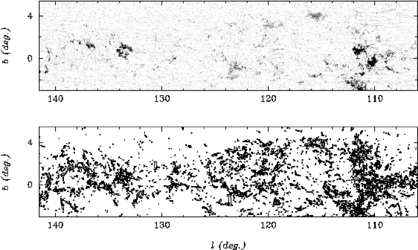
Figure 1: (top) An image of ¹²CO J=1-0 integrated intensity over the velocity interval -110 to -20 ${\rm km~{}s}^{-1}$from the FCRAO CO Survey of the outer Galaxy (Heyer et al. 1998). The halftone ranges from 0 (white) to 20 (black) K km s^-1. (bottom) The positions, sizes, and orientations of identified objects approximated as ellipses.

The decomposition extracts both isolated molecular clouds and clumps within larger cloud complexes which are identified separately due to the spatial and kinematic inhomogeneity of the molecular interstellar medium. Any element within the data cube can only be assigned to a singular object. Figure 1 shows an image of integrated intensity over the velocity range -110 to -20 ${\rm km~{}s}^{-1}$ and the ensemble of identified objects whose positions, inferred sizes and orientations are represented as ellipses with parameters $\rm l_{max}$, $\rm l_{min}$, and $\theta$.

2.2 Selection Effects

Prior to the examination of cloud properties, it is necessary to establish known selection effects. The primary selection effects are due to the limited spectral resolution of the observations, the antenna temperature threshold, and the requirement that an object be comprised of at least 5 spatial pixels (see Appendix A). The antenna temperatures of two contiguous spectroscopic channels are required to be larger than the main beam temperature threshold of 1.4 K in order for these channels to be associated with an object. Therefore, the cloud catalog does not include molecular regions with narrow ($\sigma_{v}$ $<$ 0.4 ${\rm km~{}s}^{-1}$) velocity dispersions. In Appendix B, we evaluate the sensitivity and accuracy of the method from the cloud decomposition of simple cloud models with varying signal to noise and line width. The decomposition can recover velocity dispersions as small as 0.65 ${\rm km~{}s}^{-1}$ to within 10% accuracy for signal to noise ratios greater than 4. The results are important not only to gauge the selection of objects but to evaluate the cloud scaling laws discussed in $\S$3.

Given the antenna temperature threshold of 1.4 K and assuming that ¹²CO is universally optically thick, the decomposition can not recover regions with extreme subthermal excitation conditions averaged over the angular extent of the cloud. The intensity threshold and spectroscopic channel requirements correspond to an H₂ column density of 4$\times$10²⁰ cm^-2 (see $\S$2.4) at which self shielding of CO molecules may not be effective (van Dishoeck & Black 1988). Therefore, the edges defined by this threshold likely correspond to a photodissociation boundary of CO. The distribution of ${\rm H}_{2}$ gas is likely more extended than the CO. Independent of excitation, the catalog would not include small, compact clouds with mean angular radii less than $\sim$2 arcminutes due to the requirement that the cloud is comprised of at least five pixels.

2.3 Detection and Completeness Limits for the Sample

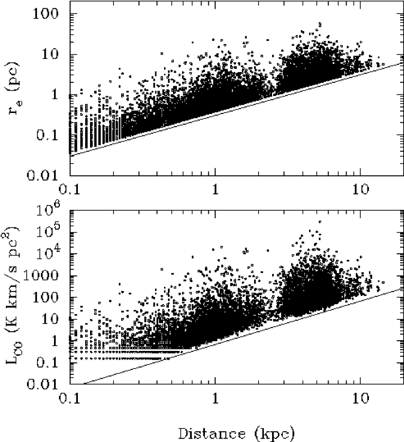
Figure 2: (top)The effective radius of identified objects as a function of kinematic distance. The lower envelope of points is due to the requirement that an object must be comprised of at least five spatial pixels. (bottom) L_CO as a function of distance. The solid line shows the minimum CO luminosity of objects in which the antenna temperature of all associated positions and spectroscopic channels is 1.4 K.

Due to the prescribed definition of a cloud, there are limits to physical quantities such as size and CO luminosity below which the cloud catalog is insensitive and incomplete. Figure 2 shows the effective cloud radius, $r_{e}=0.5\sqrt{\mbox{$\rm l_{max}$}\mbox{$\rm l_{min}$}}$ and CO luminosity as functions of the kinematic distance for all identified objects. The lower envelope of points corresponds to the minimum effective size of a cloud,

$$r_{e}^{min}(D)=10^{3}D\sqrt{\Omega_{s}N_{p}/\pi}\;\;\;pc$$

where $\Omega_{s}$ is the solid angle per pixel, D is the distance to the object in kpc, and $N_{p}$ is the minimum number of pixels per object. For this decomposition, $N_{p}=5$ so that $r_{e}^{min}=0.31D$ pc. Similarly, the minimum CO luminosity is,

$$L_{CO}^{min}(D)=N_{p}N_{c}T_{th}dv\Omega_{s}D^{2}\;\;\;K\;km\;s^{-1}\;pc^{2}$$

where $N_{c}=2$, is the minimum number of velocity channels, $dv$=0.81 ${\rm km~{}s}^{-1}$, is the spectroscopic channel width, and $T_{th}$=1.4 K is the main beam antenna temperature threshold. $L_{CO}^{min}(D)$ is shown as the solid line in Figure 2. At a distance of 10 kpc, the detection limit is 67 $K\;km\;s^{-1}\;pc^{2}$. While $L_{CO}^{min}(D)$ is the detection limit at a given distance, D, the completeness limit is higher than this value since the noise of the data contributes to the measured luminosity. The completeness limit, $L_{CO}^{c}$ is defined in this study at the 5$\sigma$ confidence as

$$L_{CO}^{c}(D)=L_{CO}^{min}+5\sigma(L_{CO})$$

where

$$\sigma(L_{CO})=\sigma dv\Omega_{s}D^{2}\sqrt{N_{c}N_{p}}\;\;\;K\;km\;s^{-1}\;pc^{2}$$

and $\sigma$=0.93 K is the median rms temperature for channels with no emission (Heyer et al. 1998). At 10 kpc, the cloud catalog is complete for CO luminosities $>$ 138 $K\;km\;s^{-1}\;pc^{2}$. This completeness limit needs to be considered when calculating power law descriptions to the CO luminosity function in $\S$2.5.1.

2.4 Application of the CO to H₂ Conversion Factor

Whenever possible, descriptions of observable quantities are presented with few or no assumptions. However, for analyses described in $\S$3.2 and $\S$4.1, it is necessary to derive total gas column densities and masses. In this investigation for which only ¹²CO observations are available, ${\rm H}_{2}$ column densities are derived using the CO to ${\rm H}_{2}$ conversion factor determined from $\gamma$-ray measurements such that

$$N(H_{2})=1.9{\times}10^{20}W_{CO}\;\;\;cm^{-2}$$

where $W_{CO}$ is the ¹²CO integrated intensity in K km s^-1 for a given line of sight (Strong & Mattox 1996). Summing over the projected area of the cloud, this corresponds to a conversion from CO luminosity, L_CO, in $K\;km\;s^{-1}\;pc^{2}$ to the total molecular mass, M_CO of the identified object,

$$M_{CO}=4.1\biggl{(}{{L_{CO}}\over{K\;km\;s^{-1}\;pc^{2}}}\biggr{)}\;\;M_{\odot}$$

which includes the factor 1.36 to account for the abundances of heavier elements (Hildebrand 1983).

The dimensional justification for a constant conversion factor is summarized by Dickman, Snell,& Schloerb (1986). The CO luminosity is the integral of the antenna temperature over all velocities and area of the cloud,

$$L_{CO}={\int}dA(l,b){\int}dvT(l,b,v)\;\;\;K\;km\;s^{-1}\;pc^{2}$$

$$L_{CO}\approx\pi r_{e}^{2}<T>{\delta}v\;\;\;\;K\;km\;s^{-1}\;pc^{2}$$

where dA is the projected area of a pixel in pc², $<T>$ is the mean brightness temperature over the projected area and velocity interval, ${\delta}v$ is the full width half maximum line width in $kms^{-1}$, and $r_{e}$ is the effective radius in pc. The gravitational parameter, $\alpha_{G}$, for a spherically symmetric, uniform density cloud is

$$\alpha_{G}\approx{{5\sigma_{v}^{2}r_{e}}\over{GM}}$$

where $\sigma_{v}$ is is the velocity dispersion of the object. Solving for ${\delta}v=\sigma_{v}(8ln2)^{1/2}$ in equation 2.8 and substituting into equation 2.7,

$$L_{CO}=1.05\pi r_{e}^{2}<T>\biggl{(}{{GM\alpha_{G}}\over{r_{e}}}\biggr{)}^{1/2}$$

Dividing equation 2.9 into $M=4/3\pi r_{e}^{3}<\rho>$, where $<\rho>$ is the mean density of the cloud yields $X_{CO}$,

$$X_{CO}={{M}\over{L_{CO}}}$$

$$X_{CO}=0.62<T>^{-1}(G{\alpha_{G}})^{-1/2}<\rho>^{1/2}$$

$$X_{CO}=4.1\biggl{(}{{<T>}\over{5K}}\biggr{)}^{-1}\biggl{(}{{<n>}\over{100cm^{-3}}}\biggr{)}^{1/2}{\alpha_{G}}^{-1/2}$$

where $<n>={\mu}m_{H_{2}}<\rho>$. The conventional assumption is that clouds are self gravitational ($\alpha_{G}\approx 1$) and the mean temperature and density do not vary from cloud to cloud such that $X_{CO}$ is constant. However, if clouds are not gravitationally bound ($\alpha_{G}>>1$), then the appropriate value of $X_{CO}$ decreases with respect to the value for a self gravitating cloud. Therefore, by applying a constant, universal value of $X_{CO}$, under the assumption that $\alpha_{G}=1$, the resultant ${\rm H}_{2}$ mass overestimates the true mass of a cloud with $\alpha_{G}>>1$.

2.5 Distributions of Measured Properties

The large number of objects identified in the decomposition of the FCRAO CO Survey of the Outer Galaxy enables a detailed examination of the CO luminosity function, the size spectrum, and line width distribution of molecular regions.

2.5.1 CO Luminosity Function

The mass spectrum of clouds, N(m)dm, within the Galaxy and clumps within molecular cloud complexes is used as a diagnostic to cloud formation and fragmentation processes (Kwan 1979); a signature of a hierarchical interstellar medium (Elmegreen & Falgarone 1996; Stutzki et al. 1998); and a guide to the initial stellar mass function (Zinnecker et al. 1993). It is typically quoted as a differential distribution which is described by a power law,

$${{dN}\over{dM}}\propto M^{-{\alpha_{M}}}\;\;\;\;\;$$

Values for $\alpha_{M}$ are similar for distributions describing clouds and cloud complexes in the Galaxy or clumps within clouds. Kramer et al. (1998) summarize the mass spectra of clumps within several cloud complexes. They find that $\alpha_{M}$ ranges from 1.6 to 1.8 over a large range of mass scales. From a sample of giant molecular clouds identified within coarsely sampled surveys of CO emission from the inner Galaxy, Sanders, Scoville & Solomon (1985) and Solomon et al. (1987) derive $\alpha_{M}=1.5$. For these Galactic surveys, the mass of a cloud is determined from the virial mass and the assumption of self gravitational equilibrium.

Figure 3 shows the differential luminosity function, ${\Delta}N/{\Delta}L_{CO}$, in equally spaced, logarithmic bins for objects with $\rm V_{\rm LSR}$$<$-20 ${\rm km~{}s}^{-1}$. The corresponding mass for a given L_CO is shown along the top x coordinate assuming a constant CO to H₂ conversion factor (see $\S$2.4). The detection limit of the sample at a distance of 10 kpc is 67 $K\;km\;s^{-1}\;pc^{2}$. The sample is complete to a limiting value of 138 $K\;km\;s^{-1}\;pc^{2}$ at a distance of 10 kpc. A power law is fit to the bins with L_CO greater than this completeness limit and weighted by $\sqrt{N}/{\Delta}L_{CO}$ where $N$ is the number of objects in each bin such that

$${{{\Delta}N}\over{{\Delta}L_{CO}}}=(3.1{\times}10^{4})L_{CO}^{-1.80\pm 0.03}(K\;km\;s^{-1}\;pc^{2})^{-1}$$

The value of the exponent is steeper than the value derived by Brand & Wouterloot (1995) for a sample of outer Galaxy clouds for which $\alpha_{M}$=1.62. This may be partly due to the improved statistics given the large number of objects and a lower luminosity completeness limit. Nevertheless, the value of the exponent is less than the critical value of 2, at which there are equal integrated luminosities (masses) over any logarithmic range of luminosity. Therefore, most of the observed flux is contributed by the most luminous objects. For example, 50% of the luminosity integrated over all identified objects (3901) comes from 35 clouds with L_CO$>$ 7800 $K\;km\;s^{-1}\;pc^{2}$ and 90% is contributed by 930 clouds with L_CO$>$ 270 $K\;km\;s^{-1}\;pc^{2}$.

2.5.2 Cloud Size Distribution

The size distribution of identified objects provides an additional measure of mean cloud properties. The differential size distribution, ${\Delta}N/{\Delta}r_{e}$, is presented in Figure 4. The detection limit at a distance of 10 kpc is shown as the vertical dotted line. A power law fit to bins above this limit and weighted by $\sqrt{N}/{\Delta}r_{e}$, yields the relation,

$${{{\Delta}N}\over{{\Delta}r_{e}}}=(1.7{\times}10^{4})r_{e}^{-3.2\pm 0.1}\;\;\;pc^{-1}$$

The size spectrum for the outer Galaxy clouds is similar to that derived from inner Galaxy surveys (Solomon et al. 1987) and targeted molecular regions over a more limited range of cloud size (Elmegreen & Falgarone 1996).

2.5.3 Line Width Distributions

Each object is characterized by a velocity dispersion, $\sigma_{v}={\delta}v/(8ln2)^{1/2}$, derived from the summed spectrum of all constituent pixels. This measure includes both line of sight motions as may be inferred from the mean line width of each profile and projected variations of the centroid velocities. Therefore, it accounts for all of the measured kinetic energy within a cloud generated by turbulence, rotation, expansion, and other dynamical processes. The distribution of velocity dispersions, $N(\sigma_{v})$, is shown in Figure 5. The decomposition is not sensitive to small line width regions and provides accurate measures for $\sigma_{v}$ $>$ 0.64 ${\rm km~{}s}^{-1}$. The distribution of velocity dispersions for clouds with large peak temperatures ($>$ 3.5 K) and presumably more accurate values of $\sigma_{v}$, shows the same shape and mean value as the distribution for all objects. The measured distribution of line width for all objects is not significantly biased by signal to noise or errors in measuring $\sigma_{v}$.

3 Cloud Scaling Relationships

With the statistics of individual properties established in the preceding sections, we now examine the relationships between various cloud properties. These relationships are motivated by the scaling laws initially identified by Larson (1981) and reexamined by many subsequent studies with varying results. These scaling laws describe 1) a power law relationship between the velocity dispersion and size of a cloud; 2) a linear correlation between the measured and virial mass of clouds; and 3) an inverse relationship between mean density and size. The three relationships are algebraically coupled such that the validity of any two of these laws necessarily implies the third (Larson 1981).

3.1 Velocity Dispersion - Size Relationship

The velocity dispersion, $\sigma_{v}$, provides a measure of the total kinetic energy in the cloud inclusive of thermal, turbulent, rotational, and expanding motions. A scaling relationship between the velocity dispersion and the size of a cloud was initially identified by Larson (1981) using data taken from the literature. A recent compilation of data from many studies using several different molecular line tracers demonstrates this correlation of velocity dispersion with size within 4 orders of magnitude in size scale (Falgarone 1996). The origin of this relationship has been attributed to turbulence (Larson 1981; Myers 1983), or simply, a consequence of gravitational equilibrium and constant gas column density which are limited by observational selection effects (Scalo 1990).

It is important to distinguish the relationship derived using multitracer observations from that determined from a single gas tracer (Goodman et al. 1998). The excitation requirements for a given molecule determine the angular extent over which any object can be identified. Multitracer observations sample different density regimes which correspond to distinct, but nested, volumes of material. In this way, a larger dynamic range of sizes is probed than can be sampled by any single gas tracer. The correlation between velocity dispersion and size has been established for single gas tracers but over a more limited range of sizes and larger intrinsic scatter (Larson 1981; Dame et al. 1987; Solomon et al. 1987). These single tracer relationships examine the variation of the velocity dispersion with size within a more limited range of density.

Figure 6 presents the variation of velocity dispersion with the effective radius, $r_{e}$, for the ensemble of clouds in this study. To more effectively consolidate the information, the mean velocity dispersion is calculated within binned cloud radii. For objects with sizes greater than $\sim$7 pc, there is a tendency for increasing velocity dispersion with size. The slope of the power law fit to objects with radii greater than 9 pc is $\sim$0.5 and similar to that derived by Solomon et al. (1987). However, the binned values show little systemic variation of the velocity dispersion with size for $r_{e}<$ 7 pc. The apparent flattening of the relationship for small clouds is not an artifact of our cloud definition since it occurs at a velocity dispersion for which our method is reasonably accurate (see Appendix B). A limited number of followup observations with much higher spectral resolution of narrow line width clouds identified in the catalog show comparable velocity dispersions (see Appendix B). A population of small clouds with line widths below our threshold for cloud identification which do follow the standard relationship can not be excluded. However, our observations have identified many small clouds with line widths in excess of the extrapolated size line-width relationship of Solomon et al. (1987). This result does not dismiss the velocity dispersion-size relationship determined from multitracer observations. Narrow line width regions within molecular clouds are identified from tracers of high density gas (NH₃, CS, HCN) and these often follow the conventional scaling law (Myers 1983). Such regions are not readily identified by ¹²CO or ¹³CO emission. Previous CO studies which have identified a size line width scaling law have been limited to large, self gravitating cloud complexes with masses greater than 10⁴ $M_{\odot}$ (Solomon et al. 1987, Scoville et al. 1987). The near constant velocity dispersion with size for the small cloud or clump population may reflect a different dynamical state than the larger giant molecular cloud complexes (see $\S$3.2).

3.2 Equilibrium of Molecular Regions

3.2.1 Survey Clouds

To evaluate the role of self gravity in the equilibrium of the identified molecular regions, we determine the magnitude of the virial mass with respect to the measured mass of the object derived from the CO luminosity. Following Bertoldi & McKee (1992), the virial mass, $M_{vir}$, is calculated from the measured cloud parameters,

$$M_{vir}={{a_{3}}\over{a_{1}a_{2}}}{{5\sigma_{v}^{2}r_{e}}\over{G}}$$

where $\sigma_{v}={\delta}v/(8ln2)^{1/2}$ is the one dimensional velocity dispersion. The constants, $a_{1}$ and $a_{2}$, measure the effects of a nonuniform density distribution and clump axial ratio, respectively, on the gravitational potential and $a_{3}$ is a statistical correction to account for the projection of an ellipsoidal cloud. These constants are evaluated using the functional forms described in Bertoldi & McKee (1992) and with the assumption of uniform density clouds ($a_{1}=1$). The value of this combination of constants, ($a_{3}/a_{1}a_{2}$), is $\sim$1. The gravitational parameter,

$$\alpha_{G}={{M_{vir}}\over{M_{CO}}}$$

provides a measure of the kinetic to gravitational energy density ratio. In the outer Galaxy catalog for which there are only ¹²CO observations, M_CO is derived assuming a CO to H₂ conversion factor. Figure 7 shows the variation of $\alpha_{G}$ with L_CO. The vertical line denotes the detection limit for L_CO at a distance of 10 kpc. The derived values of the gravitational parameter are anti-correlated with the CO luminosity. A bisector fit to the data yields the relationship

$$\alpha_{G}=53L_{CO}^{-0.49\pm 0.01}$$

with a correlation coefficient of -0.76. This expression is parameterized in terms of mass assuming a constant CO to ${\rm H}_{2}$ conversion factor,

$$\alpha_{G}=\biggl{(}{{M_{\circ}}\over{M_{CO}}}\biggr{)}^{0.49}$$

where $M_{\circ}$=1.3$\times$10⁴ $M_{\odot}$ and corresponds to the mass at which $\alpha_{G}=1$. This relationship could be due to the selection effect which excludes narrow line regions from the cloud catalog (see $\S 2.2$). The minimum value of the gravitational parameter, $\alpha_{G}^{min}$, is estimated by solving for $r_{e}$ in equation 2.7 and inserting the result into equation 2.8 such that,

$$\alpha_{G}^{min}=103\sigma_{vmin}^{3/2}<T>^{-1/2}L_{CO}^{-1/2}$$

where $\sigma_{vmin}$ is the minimum velocity dispersion recovered. For $<T>$=1.4 K and $\sigma_{v}$=0.43 ${\rm km~{}s}^{-1}$,

$$\alpha_{G}^{min}=25L_{CO}^{-1/2}$$

and is shown as the heavy line in Figure 7. The functional form of $\alpha_{G}^{min}$ provides a reasonable approximation to the lower envelope of points within the $\alpha_{G}-L_{CO}$ plane. Therefore, a population of clouds with narrow line widths, low luminosities, and smaller values of $\alpha_{G}$ could exist within the ISM but is not recovered in this decomposition. Given that there are not many points at this limit for a given value of L_CO, there may not be a significant fraction of clouds with these conditions. This selection effect is surely present in most previous studies of cloud equilibrium.

The values of L_CO and $\alpha_{G}$ are also dependent on the assumed kinematic distances to the objects. The kinematic distances in this sector of the outer Galaxy are often larger than the spectroscopic distances due to non-circular motions induced by a large scale potential (Brand & Blitz 1993). In these cases, the derived values of L_CO and therefore, M_CO, are overestimates to the true values. Therefore, the gravitational parameter is underestimated.

Finally, the variation of the gravitational parameter with L_CO can be rectified if the CO to ${\rm H}_{2}$ conversion factor is not constant but changes systematically with L_CO. Sodroski (1991) has proposed a larger value of X_CO for the outer Galaxy so that all clouds identified in that study are self gravitational. However, given the strong correlation of $\alpha_{G}$ over 4 orders of magnitude of L_CO, such an ad hoc modification to X_CO implies that the most luminous objects are collapsing. Brand & Wouterloot (1995) examined the variation of the conversion factor using ¹²CO and ¹³CO observations for a sample of far outer Galaxy clouds. Accounting for a radial gradient in ¹³CO abundance, they concluded that the conversion factor is similar to that found in the inner Galaxy. Other ¹²CO and ¹³CO studies have found no significant variation of $X_{CO}$ for outer Galaxy clouds (Carpenter, Snell, & Schloerb 1990).

The conventional assumption of a constant conversion factor is that clouds are self gravitationally bound with $\alpha_{G}\approx 1$. However, as discussed in $\S$2.4, if clouds are internally overpressured with respect to self gravity ($\alpha_{G}>>1$), then the appropriate value of $X_{CO}$ is smaller than the standard, constant value. Therefore, by using the standard value, the derived masses are upper limits and the derived values for $\alpha_{G}$ are lower limits. The large values of the gravitational parameter reflect the changing dynamical state of molecular regions with different mass. Only the most luminous objects identified in the Survey have sufficient mass to be bound by self gravity ($\alpha_{G}\sim$1). Regions with lower CO luminosities and mass are internally overpressured with respect to self gravity. This state is independent of whether the object is an isolated cloud or part of a larger cloud complex. A similar conclusion has been obtained for a sample of high latitude clouds and for several clouds in the solar neighborhood (Magnani, Blitz, & Mundy 1985; Keto & Myers 1986; Bertoldi & McKee 1992; Falgarone, Puget, & Perault 1992; Dobashi et al. 1996; Yonekura et al. 1997; Kawamura et al. 1998). The results presented here provide statistical confirmation of these earlier studies over a larger range of cloud and clump masses.

3.2.2 Targeted Regions with ¹³CO Observations

In order to gauge the results of the previous section with a more reliable tracer of molecular hydrogen mass, we have analyzed ¹²CO and ¹³CO data of targeted molecular cloud regions which lie within the Survey field (Heyer, Carpenter, & Ladd 1996; Deane 2000). The targeted fields include the giant molecular clouds Cep OB3, S140, NGC 7538, and W3. The ¹²CO data were decomposed into discrete objects with the same algorithm as the Survey cube. The ¹³CO integrated intensity is summed within the boundaries identified from the ¹²CO data and a mass, $M_{LTE}$, is derived assuming local thermodynamic equilibrium, a kinetic temperature of 10 K, a ¹³CO to ${\rm H}_{2}$ abundance of 10^-6 and a 1.36 correction for the abundance of Helium (Dickman 1978). The distances to each cloud are: 730 pc (Cep OB3), 910 pc (S140), 2.35 kpc (W3), and 3.5 kpc (NGC 7538). A virial mass for each object is derived from the tabulated size and ¹³CO velocity dispersion.

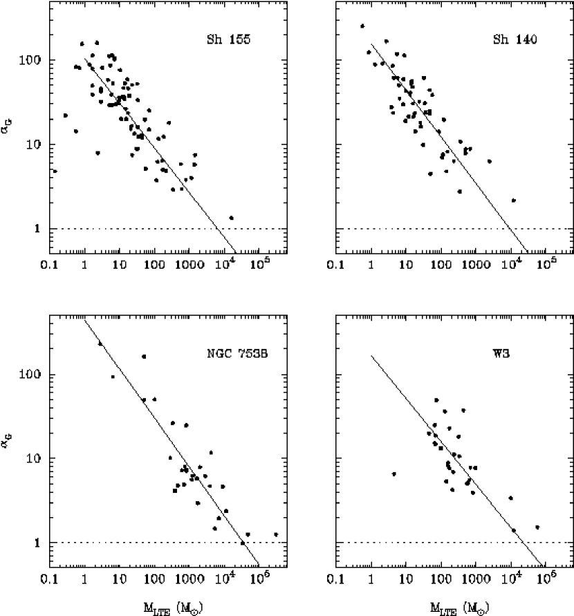
Figure 8: The variation of the gravitational parameter, $\alpha_{G}$, derived from ¹³CO observations for clumps within four targeted giant molecular cloud complexes in the outer Galaxy.

The variation of the gravitational parameter, now derived with ¹³CO measurements of molecular column density and $M_{LTE}$, is shown in Figure 8 for the four targeted giant molecular clouds. The evaluation of $\alpha_{G}$ is subject to the same selection effects as the Survey clouds such that there is the same functional dependence of $\alpha_{G}^{min}$ with $M_{LTE}$. $\alpha_{G}$ decreases with increasing luminosity and mass. Bisector fits of the data to the expression

$$\alpha_{G}=\biggl{(}{{M_{\circ}}\over{M_{LTE}}}\biggr{)}^{\epsilon}$$

where M_∘ is as defined in equation 3.4, are summarized in Table 2. Values of $\epsilon$ range between 0.51 and 0.58. For objects with masses greater than 10⁴ $M_{\odot}$, the derived values of $\alpha_{G}$ are reasonably consistent with self gravitational equilibrium. However, the lower mass clouds are highly overpressured with respect to self gravity as found for the Survey clouds.

Figure 9 shows the inferred CO to ${\rm H}_{2}$ conversion factor, $X_{CO}=M_{LTE}/L_{CO}$ as a function of $M_{LTE}$ for the identified clumps within the four fields. While there are not many objects with high mass, the scatter of the ratio for objects with $M_{LTE}>$10⁴ $M_{\odot}$ is much smaller than is found for low mass objects. The mean value for the high mass points is comparable to the value determined from $\gamma$-ray measurements (Strong & Mattox 1996). The inferred values of $X_{CO}$ for the lower mass, non-self-gravitating objects are smaller than this standard value as expected from equation 2.7. These results are direct, empirical evidence that L_CO is a reliable tracer of total mass of an object for values of L_CO $>$ 10³ K-km/s pc² but provides only an upper limit to the mass for objects with lower luminosities.

3.2.3 CO as an Tracer of H₂ Mass in Galaxies

The main isotope of CO provides the primary tracer of H₂ mass in galaxies. This utility depends upon the state of self gravitational equilibrium of the constituent clouds within the observer’s beam (Dickman, Snell, & Schloerb 1986). The non-self gravitating state of low luminosity objects does not render the use of CO as an extragalactic tracer of ${\rm H}_{2}$ mass inapplicable. Figure 3 demonstrates that much of the measured CO luminosity arises from the most massive objects within the field for which $\alpha_{G}\approx 1$. Given that L_CO provides an upper limit to the mass for non-self gravitating clouds, the mass function may be even flatter than the luminosity function. For most available resolutions of a galaxy, the large, most luminous objects would contribute most of the detected flux. Therefore, if the distribution of clouds in other galaxies is similar to the outer Galaxy, then ¹²CO remains a reliable tracer of ${\rm H}_{2}$ mass. The fractional contribution to the measured CO luminosity from the small, non self gravitating population of clouds would simply add to the scatter of inferred molecular hydrogen masses as this contribution could vary with position in a galaxy or from one galaxy to another.

3.3 Surface Densities

The third scaling relationship states that the mass surface density of molecular clouds is constant. To evaluate this relationship with the Survey clouds, the variation of CO luminosity normalized to the cloud area (or equivalently, the mean value of integrated CO intensity) with effective cloud radius is shown in Figure 10. A similar relationship is shown from the sample of objects identified in the four targeted clouds. Given the results of $\S$3.2.1, the corresponding mass surface densities are only valid for the large ($>$10 pc) objects. There is little variation of the mean integrated intensity for small clouds ($r_{e}<$10 pc) which also corresponds to the population of non self gravitating clouds. This is in part due to the method to identify clouds at a given threshold of antenna temperature and that most of the luminosity arises from the extended, lines of sight with small antenna temperatures. For these small clouds, L_CO effectively measures the projected area. For clouds with effective radii greater than 10 pc, there is weak trend for larger mean intensities with increasing size. The mass surface density of objects is determined from the ¹³CO observations of the four targeted clouds as shown in Figure 10. The mean surface density is 9 M_⊙ pc^-2 although the scatter is large for a given size. It is interesting to note that despite the uniformity of mean ¹²CO intensity between clouds or clumps, the mean column density of clumps within a cloud can vary widely. Thus, the mass surface density is not a constant of molecular clouds.

4 Discussion

The preceding sections demonstrate the non self gravitating state of molecular regions as defined by ¹²CO emission with masses less than 10³ $M_{\odot}$ while clouds with masses greater than 10⁴ $M_{\odot}$ are self gravitating. The limited accuracy of $\alpha_{G}$ precludes a definitive evaluation of the equilibrium state for regions with masses between 10³ and 10⁴ $M_{\odot}$ for which $1<\alpha_{G}<4$. Due to the high opacity of the CO J=1-0 transition, CO observations are not sensitive to the full range of molecular gas column densities known to be present in clouds. Therefore, this result does not preclude the presence of small, self gravitating regions with densities greater than 10⁴ ${\rm cm}^{-3}$ in which star formation may occur. Indeed, star formation is present within many of the small clouds of the W3/4/5 cloud complex (Carpenter, Heyer, & Snell 2000). Given the luminosity function in Figure 3, the small cloud and clump populations do not account for a significant fraction of the molecular mass in the Galaxy. Nevertheless, these molecular regions provide insight to the dynamical state of the interstellar medium. The identified objects are strictly regions where CO is detected but the dominant molecular constituent, ${\rm H}_{2}$, could extend beyond these boundaries. Moreover, these regions are embedded within a larger, atomic medium such that the boundaries represent a change in gas phase rather than sharp volume or column density variations.

Regions with large values of $\alpha_{G}$ are either short lived or are bound by external pressure and long lived with respect to the dynamical time scales. These observations can not distinguish whether a given region is bound by external pressure as this requires an examination of the thermal and dynamical state of the surrounding medium. In the absence of sufficient external pressure, these regions expand until the internal pressure is balanced by that of the external medium. In this larger configuration, the molecular gas may dissociate due to less effective self-shielding. Effectively, the CO emitting regions would be rapidly dispersed over a dynamical time along the minimum cloud dimension ($l_{min}/2\sigma_{v}$), or 5-50$\times$10⁴ years. Numerical simulations of magnetohydrodynamic turbulence in the dense interstellar medium show localized, density enhancements that would rapidly lose identity due to shear, merging with nearby clouds, or expansion into the larger medium (Ballesteros-Paredes, Vazquez, & Scalo 1999). These numerical studies would suggest that the overpressured objects identified in our survey are transient features.

However, there is indirect evidence to suggest that the internal motions of these regions are bound by some confining agent. The age of any molecular object is constrained by the time required to chemically evolve diffuse, atomic material to nominal abundances to enable a CO observation. For densities of 10² ${\rm cm}^{-3}$, this time scale is greater than 10⁶ years (Jura 1975) which is longer than the dynamical time for these objects. Unless these overpressured molecular clouds are formed within high density regions, there is simply insufficient time to chemically evolve material to reasonable abundance values. Secondly, while the lower envelope of points in Figure 7 may be defined by selection effects, the upper envelope of values of $\alpha_{G}$ systematically varies through 3 decades of cloud mass (see Figure 7). For transient, unbound objects, one would expect $\alpha_{G}>>1$ and independent of mass such that the observed correlation is unlikely. Bertoldi & McKee (1992) evaluate $\alpha_{G}$ in terms of the Bonner-Ebert mass,

$$\alpha_{G}\propto\biggl{(}{{M_{BE}}\over{M}}\biggr{)}^{2/3}$$

where

$$M_{BE}=1.182{{\sigma_{v}^{4}}\over{(G^{3}P_{\circ})^{1/2}}}$$

$$M_{BE}=2900\biggl{(}{{\sigma_{v}}\over{1km/s}}\biggr{)}^{4}\biggl{(}{{P_{\circ}/k}\over{10^{4}cm^{-3}K}}\biggr{)}^{-1/2}$$

where $P_{\circ}$ is the external pressure. The relationship between $\alpha_{G}$ and M_CO=$X_{CO}$L_CO identified in Figure 7 is shallower than that predicted assuming a constant Bonner-Ebert mass within a given complex as considered by Bertoldi & McKee (1992) although this is in part, due to a selection effect which excludes regions with small velocity dispersions. This may also be due to the spatial variation of pressure throughout the outer Galaxy and the underestimate of the gravitational parameter for lower mass objects (see $\S$2.4 and $\S$3.3). The index is similar to values derived from ¹³CO observations of targeted cloud complexes. The results of Dobashi et al. (1996), Yonekura et al. (1997), and Kawamura et al. (1998) show even shallower slopes (0.2-0.3).

4.1 Required External Pressures

The preceding sections demonstrate that there are a large number of molecular regions whose internal motions are not bound by self gravity. To remain bound in the observed configuration, these motions must be confined by the pressure of the external medium. To gauge the magnitude of the required external pressures, the full virial theorem is rewritten,

$${{\sigma_{v}^{2}}\over{l_{min}}}={{P_{\circ}}\over{k}}{{k}\over{m_{H_{2}}}}{{1}\over{N_{H_{2}}}}+{{a_{1}a_{2}}\over{a_{3}}}{{\pi Gm_{H_{2}}}\over{5}}N_{H_{2}}$$

where $\rm l_{min}$ is the measured minor axis length, $P_{\circ}$ is the external pressure, and $N_{H_{2}}$ is the mean molecular column density over the surface of the object. This expression assumes that the clouds are prolate. Figure 11 shows the quantity, $\sigma_{v}^{2}/l_{min}$ plotted as a function of $N_{H_{2}}$ for each identified object. Also shown are the variations of $\sigma_{v}^{2}/l_{min}$ with column density for different values of the external pressure for bound objects. Self gravitating objects lie along the curve P/k=0. The primary cluster of points lie well off this line. The distribution of required pressure is shown in Figure 12. The mean and median of the distribution are 1.4$\times$10⁴ and 6700 cm${}^{-3}\;K$ respectively. No significant variation of the required pressure with galactocentric radius can be determined given the limited dynamic range of $R_{gal}$ and the small number of identified objects at $R_{gal}>$ 14 kpc.

4.2 Possible Sources of External Pressures

Given the magnitude of measured line widths, the internal pressure arises from the non thermal, turbulent motions of the gas. The required pressures to bind these motions are larger than the measured thermal pressures of the interstellar medium although thermal pressure fluctuations of the required magnitude are observed within a small fraction of the atomic gas volume (Jenkins, Jura, & Lowenstein 1983; Wannier et al. 1999). However, even in the case of comparable external thermal pressure, the cloud boundary can not be maintained due the anisotropy of internal, turbulent gas flow. An initial perturbation of the cloud boundary by a turbulent fluctuation generates an imbalance of the pressure force perpendicular to the surface which in turn, causes a larger distortion of the boundary (Vishniac 1983). If the molecular clouds are simply high density regions resulting from converging gas streams within a larger turbulent flow, as suggested by numerical simulations, there is an effective external ram pressure component. However, this component is similarly anisotropic and therefore, can not provide the necessary pressure to confine the entire boundary of the cloud (Ballesteros-Paredes et al. 1999). The static magnetic field applies an effective pressure, $B^{2}/8{\pi}k$, to the molecular gas and may contribute to the pressure support of the cloud. For a 5$\mu$gauss field, this pressure is 7200 $cm^{-3}\;K$ and comparable to the values required to bind the non-self-gravitating clouds observed in this study.

Bertoldi & McKee (1992) propose that the weight of the self-gravitating cloud complex squeezes the interclump medium to provide an effective mean pressure upon a constituent clump. The magnitude of this pressure, $<P_{G}>$, is equivalent to the gravitational energy density of the cloud complex, $GM_{c}^{2}/R_{c}^{4}$ where $M_{c}$ and $R_{c}$ are the mass and radius of the cloud complex respectively. They demonstrate that the magnitude of this pressure is similar to the required pressure to bind the clumps within the four targeted cloud complexes which they analyzed. If the weight of the molecular complex is a significant component to the equilibrium of clumps, then the required pressure should vary with location of the clump within the gravitational potential. In this study, the identified objects are not grouped into cloud complexes and therefore, the self gravity of the larger complex is not evaluated.

In the outer Galaxy, the surface density of atomic gas is much larger than that of the molecular material and therefore, provides an additional component to the weight upon a given clump or isolated cloud. The mean effective external pressure at the molecular gas boundary, due to the overlying atomic gas layer is

$$<P_{G}/k>=P_{e}/k+(G/k)({N_{H}\mu m_{H}})^{2}$$

where $P_{e}/k$ is the kinematic pressure at the external atomic gas boundary, and $N_{H}\mu m_{H}$ is the mass surface density of the atomic gas across the disk (Elmegreen 1989). The kinematic pressure at the atomic gas boundary is estimated from the respective surface density and velocity dispersion of gas and stars to be 8000 cm^-3 K (Elmegreen 1989). To self shield the molecular gas, the column density of atomic gas in the near vicinity of molecular material is 2$\times$10²¹ cm^-2 such that the $<P_{G}/k>\approx 1.8{\times}10^{4}$ cm^-3-K which is comparable to the magnitude of pressures shown in Figure 12. Therefore, it is plausible that the weight of the HI layer of gas or magnetic fields provide the external pressure to maintain equilibrium of the low mass molecular regions in the outer Galaxy.

5 Conclusions

A decomposition of the FCRAO CO Survey of the outer Galaxy has identified 10,156 discrete regions of molecular gas. A subset of this catalog is analyzed with $V_{LSR}<-20$ ${\rm km~{}s}^{-1}$ which includes objects within the Perseus arm and far outer Galaxy.

1. Molecular regions with masses less than 10³ $M_{\odot}$ are not self gravitational. For these regions, ${\rm H}_{2}$ masses derived from a CO to ${\rm H}_{2}$ conversion factor are upper limits.

2. The pressures required to bind the internal motions of these non self gravitating regions are 1-2$\times$10⁴ cm^-3-K. The weight of the atomic gas layer in the disk may provide this necessary pressure to maintain the equilibrium of these clouds.

3. The ¹²CO luminosity function, ${\Delta}N/{\Delta}L_{CO}$, varies as a power law,

   $${\Delta}N/{\Delta}L_{CO}\propto L_{CO}^{-1.80\pm 0.04}.$$

   However, given the non self gravitating state of low luminosity clouds, this relationship should not be used to infer a mass spectrum of molecular clouds.

4. The ¹²CO velocity dispersion of a cloud is invariant with the size for clouds with radii less than 7 pc.

We acknowledge valuable discussions with Enrique Vazquez-Semadeni, Javier Ballesteros-Paredes and Jonathon Williams. This work is supported by NSF grant AST 97-25951 to the Five College Radio Astronomy Observatory.

6 References

Ballesteros-Paredes, J., Vazquez-Semadeni, E., & Scalo, J. 1999, ApJ, 515, 286

Bally, J., Stark, A.A., Wilson, W.D., & Henkel, C. 1988, ApJ, 324, 223

Bertoldi, F. & McKee, C.F. 1992, ApJ, 395, 140

Blitz, L. & Spergel, D.N. 1991, ApJ, 370, 205

Brand, J. & Blitz, L. 1993, AA, 275, 67

Brand, J. & Wouterloot, J.G.A. 1994, AAS, 103, 503

Brand, J. & Wouterloot, J.G.A. 1995, AA, 303, 851 ApJ, 324, 248

Carpenter, J.M., Snell, R.L., & Schloerb, F.P. 1990, ApJ, 362, 147

Carpenter, J.M., Snell, R.L., & Schloerb, F.P. 1995, ApJ, 445, 246

Carpenter, J.M., Heyer, M.H., & Snell, R.L. 2000, ApJ, in press

Clemens, D.P. & Barvainis, R. 1988, ApJS, 68, 257

Dame, T. M., Ungerechts, H., Cohen, R. S., de Geus, E. J., Grenier, I. A., May, J., Murphy, D. C., Nyman, L. A., & Thaddeus, P. 1987, ApJ, 322, 706

Deane, J. 2000, Ph.D dissertation, University of Hawaii

Dobashi, K. Bernard, J.P. & Fukui, Y. 1996, ApJ, 466, 282

Dickman, R.L. 1978, ApJS, 37, 407

Dickman, R.L., Snell, R.L., & Schloerb, F.P. 1986, ApJ, 309, 326

Elmegreen, B.G. & Lada, C.J. 1977, ApJ, 214, 725

Elmegreen, B.G. 1989, ApJ, 338, 178

Elmegreen, B.G. & Falgarone, E. 1996, ApJ, 471, 816

Falgarone, E., Puget, J.-L., & Perault, M. 1992, AA, 275, 715

Falgarone, E. 1996, in Starbursts, Triggers, Nature, and Evolution eds. B. Guiderdoni & A. Kembhavi (Springer:Berlin), p. 41

Goodman, A.A., Barranco, J.A., Wilner, D.J., & Heyer, M.H. 1998, ApJ, 504, 223

Heyer, M.H., Carpenter, J., & Ladd, E.F. 1996, ApJ, 463, 630

Heyer, M.H., Brunt, C., Snell, R.L., Howe, J., Schloerb, F.P., & Carpenter, J.M. 1998, ApS, 115, 241

Hildebrand, R.H., 1983, QJRAS, 24, 267

Jenkins, E.B., Jura, M., & Lowenstein, M. 1983, ApJ, 270, 88

Jura, M. 1975, ApJ, 197, 575

Kawamura, A. Onishi, T., Yonekura,Y., Dobashi, K., Mizuno, A., Ogawa, H., & Fukui, Y. 1998, ApJS, 117, 387

Keto, E. & Myers, P.C. 1986, ApJ, 304, 466

Kramer, C., Stutzki, J., Rohrig, R., & Corneliussen, U. 1998, AA, 329, 249

Kwan, J. 1979, ApJ, 229, 567

Larson, R.B. 1981, MNRAS, 194, 809

Lizst, H.S. & Burton, W.B. 1981, ApJ, 243, 778

Magnani, L., Blitz, L., & Mundy, L. 1985, ApJ, 295, 402

Myers, P.C. 1983, ApJ, 270, 105

Sanders, D. B., Scoville, N.Z., & Solomon, P.M. 1985, ApJ, 289, 373

Sanders, D. B., Clemens, D. P., Scoville, N. Z., & Solomon, P. M. 1985, ApJS, 60, 1

Scalo, J. 1990, in Physical Processes in Fragmentation and Star Formation, eds. Capuzzo-Doletta R. et al. Reidel:Dordrecht, p. 151

Scoville, N.Z., Yun, M.S., Sanders, D. B., Clemens, D. P., & Waller, W.H. 1987, ApJ,S, 63, 821

Sodroski, T.J. 1991, ApJ, 366, 95

Solomon, P.M., Rivolo, A.R., Barrett, J., & Yahil, A. 1987, ApJ, 319, 730

Strong, A.W. & Mattox, J.R. 1996, AA, 308, L21

Stutzki, J., Bensch, F., Heithausen, A., Ossenkopf, V., & Zielinsky, M. 1998, AA, 336, 697

van Dishoeck, E. & Black, J. H., 1988, ApJ, 334, 771

Vishniac, E.T. 1983, ApJ, 274, 152

Wannier, P, Andersson, B-G., Penprase, B.E., & Federman, S.R. 1999, ApJ, 510, 291

Yonekura,Y., Dobashi, K., Mizuno, A., Ogawa, H., & Fukui, Y. 1997, ApJS, 110, 21

Zinnecker, H., McCaughrean, M.J., Wilking, B.A. 1993, in Protostars & Planets III, eds. 429

Appendix A Description of Object Parameters

Discrete objects are identified within the $T(l,b,v)$ data cube as a closed surface such that all values are greater than or equal to a singular threshold of antenna temperature. The three dimensional pixels (hereafter, voxels) are contiguous within the volume. For a given angular position, ($l_{i},b_{i}$), a minimum of 2 contiguous channels are required to exceed the threshold. In practice, the program finds a seed voxel above the threshold and then recursively checks neighboring channels and positions to build up an object. Once checked, the voxel is flagged so it would not be checked again. A minimum of 5 angular pixels are required for an object to be included in the final catalog.

An object is comprised of N angular pixels with each pixel, i, contributing $P_{i}$ spectroscopic channels. A centroid position ($l_{c},b_{c},v_{c}$) is calculated from the intensity weighted mean position within the image,

$$l_{c}={{\sum_{i=1}^{N}\sum_{j=1}^{P_{i}}T(l_{i},b_{i},v_{j})l_{i}}\over{\sum_{i=1}^{N}\sum_{j=1}^{P_{i}}T(l_{i},b_{i},v_{j})}}$$

$$b_{c}={{\sum_{i=1}^{N}\sum_{j=1}^{P_{i}}T(l_{i},b_{i},v_{j})b_{i}}\over{\sum_{i=1}^{N}\sum_{j=1}^{P_{i}}T(l_{i},b_{i},v_{j})}}$$

$$v_{c}={{\sum_{i=1}^{N}\sum_{j=1}^{P_{i}}T(l_{i},b_{i},v_{j})v_{j}}\over{\sum_{i=1}^{N}\sum_{j=1}^{P_{i}}T(l_{i},b_{i},v_{j})}}$$

A kinematic distance, D, to the object is obtained by assuming a flat rotation curve

$$D=R_{\circ}{{(cosl_{c}+\sqrt{cos^{2}l_{c}-(x^{2}-1)})}\over{cosb_{c}}}$$

where

$$x={{1}\over{1+v_{c}/\Theta_{\circ}sinl_{c}cosb_{c}}}$$

The associated galactocentric radius, R, and scale height, z, are

$$R_{gal}=xR_{\circ}$$

$$z=Dsin(b_{c})$$

To parameterize the internal motions within an object, we calculate the equivalent width from the composite spectrum of the object.

$${\delta}v=\sum_{j=P_{min}}^{P_{max}}\psi(v_{j})dv/MAX(\psi(v_{j}))$$

where

$$\psi(v_{j})=\sum_{i=1}^{N}T(l_{i},b_{i},v_{j})$$

and $P_{min}$ and $P_{max}$ are the minimum and maximum spectroscopic contributing channels over all the pixels. ${\delta}v$ is an approximation to the full width half maximum line width of a centrally peaked spectrum. It includes motions along the line of sight as measured by the width of individual line profiles and more macroscopic motions from the variations of the centroid velocity over the projected surface of the object. This latter component is also tabulated directly,

$${\delta}v_{c}=\sqrt{8ln2}*\sqrt{\sum_{i=1}^{N}(V_{LSR}^{i}-v_{c})^{2}/(N-1)}$$

Given the complex distribution of ¹²CO emission, we have made estimates to object sizes, axial ratios, and orientations from simple measures of the associated pixels which comprise an object. The long dimension, $\rm l_{max}$, of an object is determined from the two vertices, $(l_{i},b_{i}),(x_{j},y_{j})$, with the largest angular separation,

$$l_{max}=10^{3}\Omega^{1/2}D(MAX(\sqrt{(l_{i}-x_{j})^{2}+(b_{i}-y_{j})^{2}}))\;\;\ pc$$

A mean, minimum distance, $\rm l_{min}$, is derived such that,

$$\pi l_{max}l_{min}/4=10^{6}N\Omega D^{2}\;\;\;pc^{2}$$

The orientation of the cloud within the Galaxy, $\theta$, is the angle of the major axis with respect to the positive latitude axis, measured clockwise. Obviously, this angle is only meaningful for those objects with large axial ratios, $\rm l_{max}$/$\rm l_{min}$.

The CO luminosity, L_CO, is calculated directly from the associated voxels and the kinematic distance to the object,

$$L_{CO}=10^{6}\Omega D^{2}{\delta}v\sum_{i=1}^{N}\sum_{j=1}^{P_{i}}T(l_{i},b_{i},v_{j})\;\;\;K\;km\;s^{-1}\;pc^{2}$$

Finally, the peak antenna temperature from all of the associated voxels is tabulated,

$$T_{p}=MAX[T(l_{i},b_{i},v_{j})]\;\;\;for\;\;i=1,N\;\;and\;\;j=1,P_{i}$$

Appendix B Recovery of Line Widths

To gauge the accuracy and limitations of the derived line widths of an object, we have applied the cloud decomposition algorithm to a set of model clouds with varying velocity dispersion and signal to noise. Each model cloud is described by a gaussian distribution along the angular and spectroscopic coordinates an amplitude, T_∘ such that

$$T(x,y,v)=T_{\circ}exp(-2.77(x/R_{x})^{2})exp(-2.77(y/R_{y})^{2})exp(-2.77(v/{\delta}v_{t})^{2})+T_{N}$$

where $R_{x}$ and $R_{y}$ are the full width half maximum sizes of the cloud, ${\delta}v_{t}$ is the full width half maximum line width, and $T_{N}$ is extracted from a distribution of gaussian noise with variance, $\sigma^{2}$. The size of the model cloud is fixed with $R_{x}=R_{y}=5$ pixels. The centroid velocity is held constant with respect to the angular coordinates so all of the velocity dispersion is due to the intrinisic line width of the line profiles. Models are generated with ${\delta}v_{t}$ ranging from 1.0 to 3.5 ${\rm km~{}s}^{-1}$ and varying signal to noise. Ten realizations for each cloud are constructed with a different noise field generated from a new random number seed.

The decomposition program is applied to this model data cube with a threshold of 1.5$\sigma$ as in the analysis of the Survey. Figure 13 shows the variation of the ratio of measured full width half maxium line to the intrinsic line width as a function of the intrinsic line width for models with signal to noise ratios of 5 and 10. For intrinsic line widths greater than 1.5 ${\rm km~{}s}^{-1}$, this ratio approaches unity with increasing signal to noise. The measured values are underestimated by $\sim$15%. For intrinsic line widths of 1.5 ${\rm km~{}s}^{-1}$, the measured values are overestimated by 10% and do not appear to asymtotically approach the intrinsic widths for increasing signal to noise. Finally, for intrinsic widths of 1.0 ${\rm km~{}s}^{-1}$, the spectra are not resolved by the spectrometer. Objects with such narrow line widths can only be identified for signal to noise ratios greater than 6. The velocity dispersions are well determined for regions with peak antenna temperatures greater than 4$\sigma$ and intrinsic FWHM line widths greater than 1.5 ${\rm km~{}s}^{-1}$.

As a secondary measure to the accuracy to which the velocity dispersion is recovered, we have reobserved several small clouds identified in the cloud catalog with much higher spectral resolution (0.05 ${\rm km~{}s}^{-1}$) and angular sampling ($\sim$22″). The clouds were selected to be small and to cover a limited range of line widths, ${\delta}v_{m}$. For each new map, a line width is calculated from the average spectrum and is presumed to provide an accurate measure of the true line width, ${\delta}v_{t}$ for each cloud. The results are shown as the solid circles in Figure 13. While limited in number, these measurements confirm our ability to recover the line widths for ${\delta}v>$ 1.4 ${\rm km~{}s}^{-1}$.

Figure 3: The CO luminosity function, ${\Delta}N/{\Delta}L_{CO}$ for 3901 identified objects. The top x coordinate shows the corresponding mass scales assuming a constant CO to H₂ conversion factor. The vertical dotted line denotes the detection limit of L_CO and the vertical dashed line marks the completeness limit of L_CO at a distance of 10 kpc. The power law fit to bins above the completion limit (solid line) is ${\Delta}N/{\Delta}L_{CO}$ $\propto$ L_CO^-1.80±0.03.

Figure 4: The size distribution, ${\Delta}N/{\Delta}r_{e}$, for the identified objects. The detection limit of r_e at a distance of 10 kpc is 3.1 pc. The power law fit to bins above this limit (solid line) is ${\Delta}N/{\Delta}r_{e}$ $\propto$ r${}_{e}^{-3.2\pm 0.1}$.

Figure 5: The number distribution, N($\sigma_{v}$) of measured velocity dispersion. The heavy solid shows the distribution of velocity dispersion for objects with a peak antenna temperature $>$ 3.5 K for which the velocity dispersions are well determined.

Figure 6: The variation of measured velocity dispersion, $\sigma_{v}$, and effective size, $r_{e}$. The light line shows the mean value within logarithmic bins of $r_{e}$ and the error bars reflect the dispersion of values about the mean in each bin. The heavy line shows the power law fit to the clouds with $r_{e}>$ 9 pc. The slope of the power law is similar to that found by Solomon et al. (1987). The horizontal dashed line shows the velocity dispersion to which the measured values are accurate to within 15%.

Figure 7: The variation of the gravitational parameter, $\alpha_{G}$, with CO luminosity. The dotted vertical line denotes the detection limit of L_CO at a distance of 10 kpc. The heavy line shows the minimum value of $\alpha_{G}$ to which the decomposition is sensitive due to the observational selection effect which excludes narrow line clouds.

Figure 9: The derived CO to ${\rm H}_{2}$ conversion factor for clumps identified within the cloud complexes as a function of mass. For objects with $\alpha_{G}{\approx}1$, $X_{CO}$ is comparable to the value derived from $\gamma$-ray measurements.

Figure 10: (top) The variation of mean CO integrated intensity averaged over the area of the cloud with the effective cloud radius for the sample of Survey clouds. (middle) The variation of mean CO integrated intensity averaged over the area of the cloud with the effective cloud radius for the sample of targeted clouds. (bottom) The mass surface density of objects within the targeted clouds derived from ¹³CO observations.

Figure 11: Values of $\sigma_{v}^{2}/l_{min}$ vs the mean column density for the identified objects. The solid lines show the variation of this value for varying external pressures for bound objects.

Figure 12: The distribution of required external pressures to bind the internal motions of identified molecular regions.

Figure 13: The variation of the ratio of measured to intrinsic line widths as a function of the intrinsic line width derived from a sample of model clouds with signal to noise ratios of 5 (solid line) and 10 (dashed line). The filled circles show this ratio derived from high resolution, high sampling observations of four Survey clouds.

Table 1: Derived Properties of Identified Objects

This table is available only on-line as a machine-readable table

Table 2: Fitted Parameters to $\alpha_{G}=(M_{\circ}/M)^{\epsilon}$

Complex	$\epsilon$	$M_{\circ}$
		(M⊙)
Sh 140	0.55 $\pm 0.03$	9500
Cep OB3	0.53 $\pm 0.01$	6500
W3	0.51 $\pm 0.01$	2.3$\times$104
NGC 7538	0.58 $\pm 0.04$	3.6$\times$104
Survey Clouds	0.49 $\pm 0.03$	1.1$\times$104