Astrophysical Limits on Massive Dark Matter

Abstract

Annihilations of weakly interacting dark matter particles provide an important signature for the possibility of indirect detection of dark matter in galaxy halos. These self-annihilations can be greatly enhanced in the vicinity of a massive black hole. We show that the massive black hole present at the centre of our galaxy accretes dark matter particles, creating a region of very high particle density. Consequently the annihilation rate is considerably increased, with a large number of $e^{+}e^{-}$ pairs being produced either directly or by successive decays of mesons. We evaluate the synchrotron emission (and self-absorption) associated with the propagation of these particles through the galactic magnetic field, and are able to constrain the allowed values of masses and cross sections of dark matter particles.

1 Introduction

There is convincing evidence for the existence of an unseen non-baryonic component in the energy-density of the universe. The most promising dark matter candidates appear to be weakly interacting massive particles (WIMPs) and in particular the so-called neutralinos, arising in supersymmetric scenarios as well as much heavier particles (WIMPzillas) which could have been produced non-thermally in the early universe (for a review of particle candidates for dark matter see e.g. Ellis (1998)).

The annihilations of these X-particles would generate quarks, leptons, gauge and Higgs bosons and gluons. Consequently $e^{+}e^{-}$ pairs would be produced either directly or by successive decays of mesons, and they are expected to lose their energy through synchrotron radiation as they propagate in the galactic magnetic field. This radiation is expected to be greatly enhanced in the proximity of the galactic centre, where the existence of a massive black hole creates a region of very high dark matter particle density and consequently a great increase in the annihilation rate and synchrotron radiation.

We discuss in section 2 the distribution of dark matter particles in our galaxy and in particular around the central black hole, following Gondolo & Silk (1999) (from now on, Paper I). In section 3 we evaluate the annihilation $e^{+}e^{-}$ spectrum and their synchrotron emission. Finally in section 4 we discuss our results and determine the regions of the mass-annihilation cross section plane which give predictions compatible with experimental data.

2 Dark matter distribution around the galactic centre

There is strong evidence for the existence of a massive compact object lying within the inner $0.015\rm pc$ of the galactic centre (see Yusef-Zadeh, Melia & Wardle (2000) and references therein). This object is a compelling candidate for a massive black hole, with mass $M=(2.6\pm 0.2)\times 10^{6}M_{\odot}$. The galactic halo density profile is modified in the neighborood of the galactic centre from the adiabatic process of accretion towards the central black hole. If we consider an initially power-law type profile of index $\gamma$, similar to those predicted by high resolution N-body simulations (Navarro, Frenk & White 1997; Ghigna et al. 2000), the corresponding dark matter profile after accretion is, from paper I

$$\rho^{\prime}=\left[\alpha_{\gamma}\left(\frac{M}{\rho_{D}D^{3}}\right)^{3-\gamma}\right]^{\gamma_{sp}-\gamma}\rho_{D}\;g(r)\left(\frac{D}{r}\right)^{\gamma_{sp}}$$ (1)

where $\gamma_{sp}=(9-2\gamma)/(4-\gamma)$, $D$ is the solar distance from the galactic centre and $\rho_{D}=0.24GeV/c^{2}/cm^{3}$ is the density in the solar neighbourhood. The factors $\alpha_{\gamma}$ and $g_{\gamma}(r)$ cannot be determined analytically (for approximate expressions and numerical values see paper I). The expression (1) is only valid in a central region of size $R_{sp}=\alpha_{\gamma}D(M/\rho_{D}D^{3})^{1/(3-\gamma)}$ where the central black hole dominates the gravitational potential.

If we take into account the annihilation of dark matter particles, the density cannot grow to arbitrarily high values, the maximal density being fixed by the value

$$\rho_{core}=m/\sigma vt_{BH}$$ (2)

where $t_{BH}\approx 10^{10}years$ is the age of the central black hole. The final profile, resulting from the adiabatic accretion of annihilating dark matter on a massive black hole is

$$\rho_{dm}(r)=\frac{\rho^{\prime}(r)\rho_{core}}{\rho^{\prime}(r)+\rho_{core}}$$ (3)

following a power law for large values of r, and with a flat core of density $\rho_{core}$ and dimension

$$R_{core}=R_{sp}\left(\frac{\rho(R_{sp})}{\rho_{core}}\right)^{(1/\gamma_{sp})}$$ (4)

3 Constraints from Synchrotron Emission

Among the products of annihilation of dark matter particles, there will be electrons and positrons, which are expected to produce synchrotron radiation in the magnetic field around the galactic centre. The $e^{+}e^{-}$ component produced by the hadronic jets has been computed using the MLLA approximation.

The galactic magnetic field can be described using the ’equipartition assumption’, where the magnetic, kinetic and gravitational energy of the matter accreting on the central black hole are in approximate equipartition (see Melia (1992)). In this case the magnetic field can be expressed as

$$B(r)=1\mu G\left(\frac{r}{pc}\right)^{-5/4}$$ (5)

Figure 1: Values of $Y_{e}$ as a function of particle mass.

Energy-loss length scale.

As we shall see, most of the annihilations happen at very small distances from the centre, typically at $\approx min(R_{core},10Rs)$, i.e. in a region with magnetic fields of the order of $>1G$. Under these conditions, comparable to the size of the region where most of the annihilations occur, the electrons lose their energy almost in place. To see this, consider the critical synchrotron frequency $\nu_{c}(E)$ i.e. the frequency around which the synchrotron emission of an electron of energy E, in a magnetic field of strength B, peaks, namely

$$\nu_{c}(E)=\frac{3}{4\pi}\frac{eB}{m_{e}c}\left(\frac{E}{m_{e}c^{2}}\right)^{2}\,.$$ (6)

Inverting this relation, we find the energy of the electrons which give the maximum contribution at that frequency,

$$E_{m}(\nu)=\left(\frac{4\pi}{3}\frac{m_{e}^{3}c^{5}}{e}\frac{\nu}{B}\right)^{1/2}=0.25\left(\frac{\nu}{\mbox{MHz}}\right)^{1/2}\left(\frac{r}{\mbox{pc}}\right)^{5/8}\mbox{GeV}$$ (7)

Figure 2: Left panel: $A_{\nu}$ as a function of frequency for $m_{X}=1$TeV. The two upper curves correspond to the cross section $\sigma v\approx 10^{-28}/m_{X}^{2}(\rm GeV)\,\rm cm^{3}s^{-1},$ close to the unitarity limit; the two lower curves correspond to $\sigma v\approx 10^{-38}/m_{X}^{2}(\rm GeV)\,\rm cm^{3}s^{-1},$ a cross section more typical for wimps. Results for two values of the density profile are shown in each case: $\gamma=1$ (solid curves) and $\gamma=1.5$ (dashed curves). Right panel: $A_{\nu}$ as a function of the particle mass for $\nu$=408MHz, $\sigma v=10^{-10}/m_{X}^{2}$ (in physical units) and two values of $\gamma$.

The typical synchrotron loss length for an energy corresponding to $E_{m}(\nu)$ can be expressed as a function of the distance $r$ from the central black hole for the magnetic field profile in Eq. (5):

$$l_{e}(E_{m}(\nu))=\left(\frac{27}{16\pi}\right)^{1/2}\left(\frac{m_{e}^{5}c^{11}}{e^{7}}\right)^{1/2}\frac{1}{\nu^{1/2}}\frac{1}{B^{3/2}}$$

$$=1.025\cdot 10^{10}\left(\frac{\nu}{\mbox{MHz}}\right)^{-1/2}\left(\frac{r}{\mbox{pc}}\right)^{15/8}\mbox{pc}$$ (8)

For a frequency of 408 MHz, which produces, as we shall see, the most stringent upper bound on the Galactic Centre emission, we get

$$l_{e}(E_{m}(\nu))=5.074\cdot 10^{8}\left(\frac{r}{\mbox{pc}}\right)^{15/8}\mbox{pc}$$ (9)

The diffusion length $D=D(B(r),E)$, which can be approximated as a third of the radius of gyration of the electron, is given by

$$D(E_{m}(\nu))=\frac{E}{3eB}\approx 8.991\cdot 10^{-8}\left(\frac{\nu_{c}}{\mbox{MHz}}\right)^{1/2}\left(\frac{r}{\mbox{pc}}\right)^{15/8}\mbox{pc}$$ (10)

Since $l_{e}(E_{m}(\nu))>>D(E_{m}(\nu))$ for all practically relevant parameters, an electron will diffuse a distance $\sqrt{l_{e}D}$ before it loses most of its energy. Numerically,

$$\frac{\sqrt{l_{e}D}}{r}\approx 3.035\cdot 10^{1}\left(\frac{r}{\mbox{pc}}\right)^{7/8}$$ (11)

or, expressing the distance as a function of the Schwarzschild radius

$$\frac{\sqrt{l_{e}D}}{r}\approx 7.059\cdot 10^{-5}\left(\frac{r}{R_{s}}\right)^{7/8}$$ (12)

We can thus assume that the electrons lose their energy practically in place.

Figure 3: Comparison of Sgr A* (see Narayan et al. (1998)) observed spectrum with expected fluxes. The values of particle mass and cross section were choosen to fit the experimental data normalisation.

Electron Production Spectrum.

To compute the synchrotron luminosity produced by the propagation of $e^{\pm}$ in the galactic magnetic field, we need to evaluate their energy distribution in the magnetic field which is given by (see Gondolo (2000))

$$\frac{dn}{dE}=\frac{\Gamma Y_{e}(>E)}{P(E)}f_{e}(r)$$ (13)

where $\Gamma$ is the annihilation rate

$$\Gamma=\frac{\sigma v}{m_{x}^{2}}\int_{0}^{\infty}\rho_{sp}^{2}4\pi r^{2}\;\;dr\,.$$ (14)

The function $f_{e}(r)$ is given by

$$f_{e}(r)=\frac{\rho_{sp}^{2}}{\int_{0}^{\infty}\rho_{sp}^{2}4\pi r^{2}\;\;dr}$$ (15)

and

$$P(E)=\frac{2e^{4}B^{2}E^{2}}{3m_{e}^{4}c^{7}}$$ (16)

is the total synchrotron power spectrum. Note that the general expression for $f_{e}(r)$ would have to take into account spatial redistribution by diffusion (see e.g. Gondolo (2000)), which we demonstrated to be negligible in our model.

The quantity $Y_{e}(>E)$ is the number of $e^{+}e^{-}$ with energy above E produced per annihilation, which depends on the annihilation modes. Eq. (7) shows that for the frequencies we are interested in, $E_{m}(\nu)<<m_{X}$, and thus the energy dependence of $Y_{e}(>E)$ can be neglected. We will estimate $Y_{e}(>E)$ by the number of charged particles produced in quark fragmentation (see footnote); in figure 1 we show the values of Y as a function of the particle mass.

Synchrotron Luminosity.

For each electron the total power radiated in the frequency interval between $\nu$ and $\nu+d\nu$ is given by

$$P(\nu,E)=\frac{\sqrt{3}e^{3}}{m_{e}c^{2}}B(r)\frac{\nu}{\nu_{c}(E)}\int_{0}^{\infty}K_{5/3}(y)dy$$

$$=\frac{\sqrt{3}e^{3}}{m_{e}c^{2}}B(r)F\left(\frac{\nu}{\nu_{c}(E)}\right)$$ (17)

where we introduced

$$F\left(\frac{\nu}{\nu_{c}(E)}\right)=\frac{\nu}{\nu_{c}(E)}\int_{0}^{\infty}K_{5/3}(y)dy$$ (18)

Integrating this formula we obtain the total synchrotron luminosity

$$L_{\nu}=\int_{0}^{\infty}dr\;\;4\pi r^{2}\int_{m_{e}}^{m_{x}}dE\;\;\frac{dn_{e}}{dE}P(\nu,E)$$ (19)

which by substitution becomes

$$L_{\nu}=\frac{\sqrt{3}e^{3}\Gamma}{m_{e}c^{2}}\int_{0}^{\infty}dr4\pi r^{2}f_{e}(r)B(r)\int_{m_{e}}^{m_{x}}dE\frac{Y_{e}(>E)}{P(E)}F\left(\frac{\nu}{\nu_{c}(E)}\right)$$ (20)

It is possible to simplify this formula by introducing the following approximation for the function $F\left(\frac{\nu}{\nu_{c}(E)}\right)$ (see Rybicki & Lightman (1979))

$$F\left(\frac{\nu}{\nu_{c}(E)}\right)\approx\delta(\nu/\nu_{c}(E)-0.29)\,.$$ (21)

The evaluation of the integral then gives

$$L_{\nu}\approx\frac{9}{8}\left(\frac{1}{0.29\pi}\frac{m_{e}^{3}c^{5}}{e}\right)^{1/2}\frac{\Gamma Y_{e}(>E)}{\sqrt{\nu}}\;I$$ (22)

where

$$I=\int_{0}^{\infty}dr\;\;4\pi r^{2}f_{e}(r)B^{-1/2}(r)$$ (23)

Synchrotron Self-Absorption.

The synchrotron self-absorption coefficent is by definition (see Rybicki & Lightman (1979))

$$A_{\nu}=\frac{1}{a_{\nu}}\int_{0}^{\infty}(1-e^{-\tau(b)})2\pi b\;\;db$$ (24)

where $\tau(b)$ is the optical depth as a function of the cylindrical coordinate b

$$\tau(b)=a_{\nu}\int_{d(b)}^{\infty}f_{e}(b,z)\;\;dz$$ (25)

and the coefficent $a_{\nu}$ is given by

$$a_{\nu}=\frac{e^{3}\Gamma B(r)}{9m_{e}\nu^{2}}\int_{m_{e}}^{m}E^{2}\frac{d}{dE}\left[\frac{Y_{e}(>E)}{E^{2}P(E)}\right]F\left(\frac{\nu}{\nu_{c}}\right)\;\;dE$$ (26)

The final luminosity is obtained by multiplying Eq. (19) with $A_{\nu}$ given by Eq. (24). It is evident that in the limit of small optical depths the coefficent $A_{\nu}\rightarrow 1$, as can be seen by expanding the exponential.

Furthermore the lower limit of integration of expression 25 is

$$d(b)=0\;\;\;\;for\;\;\;\;b^{2}+z^{2}>(4Rs)^{2}$$ (27)

$$d(b)=\sqrt{(4Rs)^{2}-b^{2}}\;\;\;\;\;elsewhere$$

Using the approximation introduced in Eq. (21) we find for $a_{\nu}$ the following expression

$$a_{\nu}=\frac{\Gamma Y}{4\pi}\frac{c^{2}}{\nu^{3}},$$ (28)

which can in turn be used to evaluate $\tau(b)$ in Eq. (25) and $A_{\nu}$ in Eq. (24).

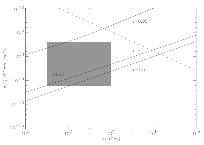
Figure 4: Exclusion plot based on the comparison between predicted flux and radio observations of the galactic centre.The 3 solid curves indicate, for different values of the density profile power law index, the lower edge of the excluded regions. The dashed line shows, for comparison, the unitarity bound, $\sigma v\simeq 1/m_{X}^{2}$. The shaded region is the portion of the parameter space occupied by cosmologically interesting neutralinos (i.e. those leading to $0.025<\Omega_{X}h^{2}<1$; see, e.g. Bergstrom, Ullio & Buckley (1997)).

Note that the synchrotron loss time-scale is proportional to $B^{-2}\propto r^{5/2}.$ We compare this with the annihilation time, which determines where the inner density drops drastically: $t_{ann}\propto r^{(9-2\gamma)/(4-\gamma)+1/2}.$ In other words, the annihilation time goes to zero more rapidly than the synchrotron loss time as $r$ goes to 0. Hence synchrotron losses are important throughout the annihilation region.

Extension to the wimpzilla mass range introduces far more uncertain physics. The wimpzilla cross sections strongly depend on new physics beyond the electroweak scale. Similarly to the case of electroweak gauge bosons, one can expect a general scaling $\sigma v\sim\alpha^{2}/m_{X}^{2}$ for the self-annihilation cross section where $\alpha\mathrel{\mathchoice{\lower 4.0pt\vbox{\halign{$\mathsurround 0pt\displaystyle\hfil#\hfil$\cr<\crcr\sim\crcr}}}{\lower 4.0pt\vbox{\halign{$\mathsurround 0pt\textstyle\hfil#\hfil$\cr<\crcr\sim\crcr}}}{\lower 4.0pt\vbox{\halign{$\mathsurround 0pt\scriptstyle\hfil#\hfil$\cr<\crcr\sim\crcr}}}{\lower 4.0pt\vbox{\halign{$\mathsurround 0pt\scriptscriptstyle\hfil#\hfil$\cr<\crcr\sim\crcr}}}}1$ is some dimensionless gauge coupling. In four dimensional field theory, the conservation of probability (unitarity) roughly corresponds to this scaling for $\alpha\to 1$ (see, e.g., Weinberg (1995)). In order to retain generality, we will therefore consider Wimpzilla annihilation cross sections in the range $\sigma v\mathrel{\mathchoice{\lower 4.0pt\vbox{\halign{$\mathsurround 0pt\displaystyle\hfil#\hfil$\cr<\crcr\sim\crcr}}}{\lower 4.0pt\vbox{\halign{$\mathsurround 0pt\textstyle\hfil#\hfil$\cr<\crcr\sim\crcr}}}{\lower 4.0pt\vbox{\halign{$\mathsurround 0pt\scriptstyle\hfil#\hfil$\cr<\crcr\sim\crcr}}}{\lower 4.0pt\vbox{\halign{$\mathsurround 0pt\scriptscriptstyle\hfil#\hfil$\cr<\crcr\sim\crcr}}}}1/m_{X}^{2}$. We note, however, that beyond four dimensional field theory, such as in theories with extra dimensions and in string theory, larger cross sections may be possible.

We first evaluate the self-absorption coefficent for selected values of the mass, as a function of frequency. The result, shown in fig.2, is a coefficent which grows from very low values (showing that absorption is important at 408 MHz) and then reaches the value 1, around a frequency which is strongly dependent on the cross section and the mass $m_{X}$, but not so much on the profile power law index $\gamma$. On the left the above coefficent is evaluated for two different values of the cross section, the first one corresponding to the maximum possible value (the so called unitary bound, see Griest & Kamionkowski (1990)) and the second one corresponding to typical cross sections one can find in supersymmetric scenarios (see, e.g., Bergstrom, Ullio & Buckley (1997)).

The right part of fig.2 shows the self-absorption coefficent at the fixed frequency of 408MHz as a function of the neutralino mass. The behaviour shown is qualitatively the same for any value of the cross-section and for different $\gamma$. In figure 3 we compare the predicted spectrum with the observations; we choose a set of parameters $m_{X}$, $\gamma$ and $\sigma v$ in order to reproduce the observed normalisation. It is remarkable that in that way one can reproduce the observe d spectrum over a significant range of frequencies. The set of dark matter parameters for which the fluxes predicted in our model are consistent with observation is shown in the exclusion plot of fig. 4. The boundaries of the excluded range represent the parameter values for which the observed flux is explained by the dark matter scenario discussed here.

4 Conclusions and perspectives

We have shown that present data on the emission from Sgr A* are compatible with quite a wide set of dark matter parameters. The evaluation of synchrotron self-absorption has enabled us to reach an alternative conclusion from an earlier claim of incompatibility of cuspy halos with the existence of annihilating wimp dark matter. Our final result is that the experimental data on Sgr A* spectrum at radio wavelengths could be explained by synchrotron emission of electrons produced in the annihilation of relatively massive dark matter particles, extending from TeV masses to $m_{X}>10^{8}\rm GeV$. The former is relevant to recent studies of coannihilation (Boehm, Djouadi & Drees (2000)), that suggest that WIMPs with $\Omega_{X}h^{2}=0.2$ can extend up to several TeV, and the latter is relevant for particles (wimpzillas) that are produced non-thermally in the primordial universe.

We have found that with the current data situation, the synchrotron emission tends to give somewhat sharper constraints on masses and cross sections than the gamma-ray fluxes (cf. Baltz et al. (2000)). This situation could be reversed by more sensitive gamma-ray observations anticipated from upcoming experiments. However the synchrotron predictions are uncertain because of our relative ignorance about the magnetic field strength near the central black hole, and gamma ray fluxes are subject to similarly uncertain amounts of self-absorption.The ANTARES neutrino experiment will eventually be able to set a relatively model-independent limit on the annihilation flux from the Galactic Centre.

References

- [1] Baltz E.A., Briot C., Salati P., Taillet R., Silk J., 2000, PRD, 61, 023514
- [2] Bergstrom L., Ullio P., Buckley J.H., 1997, astro-ph/9712318
- [3] Bhattacharjee P. & Sigl G., 2000, Phys. Rep., 327, 109, and references therein
- [4] Boehm C., Djouadi A., Drees M. , 2000 , PRD, 62, 035012
- [5] Dokshitzer Yu. L., Khoze V. A., Mueller A. H., & Troyan S. I., 1991, Basics of perturbative QCD, Editions Frontiers, Saclay
- [6] Ellis J., 1998,astro-ph/9812211
- [7] Ellis R. K., Stirling W. J., & Webber B. R., 1996, QCD and Collider Physics, Cambridge Univ. Press, Cambridge, England
- [8] Ghigna, S., Moore, B., Governato, F., Lake, G., Quinn, T. and Stadel, J. 2000, ApJ in press.
- [9] Gondolo P. & Silk J., 1999, PRL, 83, 1719
- [10] Gondolo P., 2000, astro-ph/0002226
- [11] K.Griest & M.Kamionkowski, 1990, PRL, 64, 615
- [12] Khoze V. A. & Ochs W., Int. J. Mod. Phys., 1997, A12, 2949
- [13] Melia F., 1992, ApJ, 387, L25
- [14] Navarro J., Frenk C.S. & White S.D.M., 1997, ApJ, 490, 493
- [15] Narayan et al., 1998, ApJ, 492, 554
- [16] Rybicki G.B., Lightman A.P., Radiative Processes in Astrophysics, 1979, John Wiley & Sons
- [17] S. Weinberg, 1995, The Quantum Theory of Fields Vol 1: Foundations, Cambridge University Press, Cambridge
- [18] Yusef-Zadeh F., Melia F. & Wardle M., 2000, astro-ph/0002376