Simulations of black hole–neutron star binary coalescence

Abstract

We show the results of dynamical simulations of the coalescence of black hole–neutron star binaries. We use a Newtonian Smooth Particle Hydrodynamics code, and include the effects of gravitational radiation back reaction with the quadrupole approximation for point masses, and compute the gravitational radiation waveforms. We assume a polytropic equation of state determines the structure of the neutron star in equilibrium, and use an ideal gas law to follow the dynamical evolution. Three main parameters are explored: (i) The distribution of angular momentum in the system in the initial configuration, namely tidally locked systems vs. irrotational binaries; (ii) The stiffness of the equation of state through the value of the adiabatic index $\Gamma$ (ranging from $\Gamma=5/3$ to $\Gamma=3$); (iii) The initial mass ratio $q=M_{NS}/M_{BH}$. We find that it is the value of $\Gamma$ that determines how the coalescence takes place, with immediate and complete tidal disruption for $\Gamma\leq 2$, while the core of the neutron star survives and stays in orbit around the black hole for $\Gamma=3$. This result is largely independent of the initial mass ratio and spin configuration, and is reflected directly in the gravitational radiation signal. For a wide range of mass ratios, massive accretion disks are formed ($M_{disk}\approx 0.2M_{\odot}$), with baryon–free regions that could possibly give rise to gamma ray bursts.

I Introduction

The emission of gravitational waves in a binary system will eventually drive the system to coalesce through angular momentum losses, if the decay time is less than the Hubble time. The observed decay for known binary neutron star systems such as PSR 1913+16 matches the prediction of general relativity to high accuracy (Stairs et al. 1998). There are still no observations of black hole–neutron star systems, but they are believed to exist, with corresponding coalescence rates that are comparable to those of double NS systems (see Kalogera & Belczyński, these proceedings).

These systems are candidates for detection by gravitational wave detectors such as LIGO and VIRGO. Although the final coalescence signal will probably be out of the frequency range of the first observatories, the inspiral phase, during which the stars can be thought of as point masses, will certainly be observable in this respect. For the final coalescence waveform, modeling the hydrodynamics in the system becomes an important issue, as it can affect its evolution in a significant manner. For example, Newtonian tidal effects due to the finite size of the stars, can alone de–stabilize the orbit and make it decay on a dynamical timescale (see Lai, Rasio & Shapiro 1993a).

We have studied the dynamical interactions in close black hole–neutron star binary systems previously for a variety of initial configurations (Lee & Kluźniak 1995, 1999a,b, hereafter papers I & II respectively; Lee 2000, hereafter paper III), and present here an overview of the results these simulations have produced. The results are not only relevant for the production of gravitational waves, but also for the progenitor systems of gamma ray bursts (GRBs, Kluźniak & Lee 1998; Janka et al. 1999), and the production of heavy elements through r–process nucleosynthesis (Lattimer & Schramm 1974, 1976; Symbalisty & Schramm 1982).

II Numerical method and initial conditions

II.1 Numerical method

All the computations presented here have been carried out using the Smooth Particle Hydrodynamics (SPH) method. This is a Lagrangian technique, originally developed by Lucy (1977) and Gingold & Monaghan (1977) and is ideally suited for the study of complicated flows in three dimensions, when no assumptions about symmetry in the system are made, and where there are large volumes that are basically devoid of matter. An excellent review has been given by Monaghan (1992). The code is essentially Newtonian, and makes use of a binary tree structure to find hydrodynamical forces and carry out the gravitational force computation, with a multipole expansion to quadrupole order. The viscosity is artificial, its purpose being the modeling of shocks and avoiding the interpenetration of SPH particles. We have settled on the form of Balsara (1995) for our latest work, since it minimizes the effects of shear viscosity on the evolution of the system. This is of particular importance for this work, since massive accretion disks are often formed around the black hole after the initial dynamical encounter.

The black hole is modeled as a Newtonian point mass, producing a potential

$$\Phi=-GM_{BH}/|\vec{r}-\vec{r}_{BH}|$$ (1)

at position $\vec{r}$. To model the horizon, an absorbing boundary is placed at the Schwarzschild radius $r_{Sch}=2GM_{BH}/c^{2}$. Any particle crossing this boundary is removed from the simulation. Its mass is added to that of the black hole, and the latter’s position and momentum are adjusted so as to ensure the conservation of total mass and total linear momentum in the system. The simulations shown here have used between 8,000 and 40,000 SPH particles initially. Since accretion onto the black hole entails a loss of particles, this number decreases during the simulation.

In most of the simulations presented here we have included a back reaction term to mock the effect that the emission of gravitational waves has on the evolution of the system, by draining angular momentum during the orbital evolution. This acceleration is calculated in the quadrupole approximation, assuming the two components are point masses (see e.g. Zhuge, Centrella & McMillan 1996; Davies et al. 1994; Rosswog et al. 1999). This term in the equations of motion is switched off when (and if) complete tidal disruption occurs, or if the mass of the secondary (neutron star) core drops below a certain limit (usually one tenth of the initial neutron star mass), in the cases when the star is not completely shredded by tidal forces (details of the implementation of the back reaction force can be found in Paper III).

The gravitational wave emission is calculated in the quadrupole approximation, by adding the contribution from the fluid as a whole to that of the black hole as a point mass. This gives the waveforms directly from the second derivatives of the inertia tensor. To obtain the luminosity an additional (numerical) derivative is required. For the calculation of power spectra, one can attach a point–mass inspiral signal to the coalescence waveform at earlier times, that matches smoothly at the time the dynamical simulation is started.

II.2 Initial Conditions

To perform dynamical simulations, we first construct a neutron star in hydrostatic equilibrium. The equation of state is taken to be that of a polytrope, with $P=K\rho^{\Gamma}$ ($K$ and $\Gamma$ are taken constant throughout the star). We place $N$ SPH particles on a cubic lattice, with masses proportional to the Lane–Emden density at the corresponding radius. This ensures that the spatial resolution is approximately constant, and it helps to model the edge of the star more accurately, since that is where the density gradient is often the largest, for the values of the adiabatic index $\Gamma$ that we consider. In all the calculations presented here, the neutron star has mass $M_{NS}=1.4M_{\odot}$ and radius $R_{NS}=13.4$ km. For each value of the index $\Gamma=3;2.5;2;5/3$ we find the value of $K$ that ensures this mass and radius. After placing the particles on the cubic lattice, the star is relaxed in an inertial reference frame, with an artificial damping term in the equations of motion, keeping the specific entropy constant. After relaxation, all our spherical stars satisfy the virial theorem to within one part in $10^{3}$. For the following, distances and masses are measured in units of $R_{NS}$ and $M_{NS}$, so that time and density are measured in units of $t=1.146\times 10^{-4}s(R/R_{NS})^{3/2}(M_{NS}/1.4M_{\odot})^{-1/2}$ and $\rho=1.14\times 10^{18}kg~{}m^{-3}(R/R_{NS})^{-3}(M_{NS}/1.4M_{\odot})$

The choice of a polytropic equation of state (instead of a physical equation of state such as that of Lattimer & Swesty 1991) was made in order to explore what effect the compressibility of the fluid has on the global evolution of the system, and on the gravitational wave signal. For polytropes, the mass–radius relationship is $R\propto M^{(\Gamma-2)/(3\Gamma-4)}$. So this means that for $\Gamma>2$, the neutron star will respond to mass loss by shrinking, while for $\Gamma<2$ it will expand. A star with $\Gamma=2$ has a radius that is independent of its mass. As we will show below, this has a crucial effect on the outcome of the coalescence process.

The next step in constructing the initial conditions depends on the spin of the star. Typically, the binary separation is only a few stelar radii when we begin our dynamical calculations, and so the tidal deformation of the neutron star is quite large. We consider two extreme cases of angular distribution in the system.

In the first, the star is tidally locked, so that the same side of the star always faces the black hole companion. This initial condition is easy to set up, since the system is in a state of rigid rotation. Thus we can view the binary in the co–rotating frame and neglect Coriolis forces (since we are interested in an equilibrium configuration), with an artifical damping term in the equations of motion and wait for it to relax to a static configuration. While this relaxation procedure is carried out, the orbital velocity of the co–rotating frame is continously adjusted so that the force on the center of mass of the star is exactly balanced by the centrifugal acceleration.

The second type of initial condition we consider is that of an irrotational binary. In this case, the star has essentially zero spin when viewed from an external, inertial reference frame. This is more complicated to set up, and we have used the method of Lai, Rasio & Shapiro (1993b) for our calculations. They developed a variational method to obtain a solution to this problem by approximating the star as a tri–axial ellipsoid (in this case an irrotational Roche–Riemann ellipsoid). It still experiences tidal deformations, but the shape of the star is fixed in the co–rotating frame, while internal motions with zero circulation take place in its interior.

Realistically, the first kind of initial condition was shown to be nearly impossible by Kochanek (1992) and Bildsten & Cutler (1992), because the viscosity inside neutron stars is not large enough to maintain synchronization during the inspiral phase. Essentially, the stars will coalesce with whatever spin configurations they have when inspiral begins.

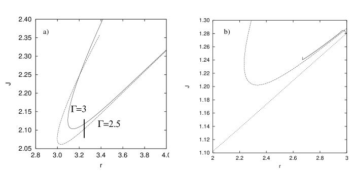
Figure 1: Total angular momentum $J$ as a function of binary separation $r$ for various black hole–neutron star binaries. (a) Irrotational binaries with $q=0.5$ and $\Gamma=3$ (solid line) and $\Gamma=2.5$ (dashed line). The thick black vertical line marks the separation used to start dynamical calculations. (b) Tidally locked binary with $\Gamma=5/3$ and $q=1$. The solid line is the result of an SPH relaxation sequence, the dashed line results from approximating the neutron star as a compressible tri–axial ellipsoid, and the dotted line from assuming it is a rigid sphere.

In either case, the fact that the stars are not point masses has a direct impact on the evolution of the system, and on its configuration immediatly before coalescence. We show in Figure 1 plots of total angular momentum $J$ in the system as a function of orbital separation for several systems. It is clear that there are important deviations from Keplerian point–mass behavior, and even from the result obtained by treating the stars as rigid spheres. The turning points in the curves show the presence of a dynamical instability, which, once reached, can drive orbital decay on a dynamical timescale (for many of the parameters in the runs shown here, this can be as fast as the decay due to the emission of gravitational waves). It is crucial to model the hydrodynamics in these systems if one is to extract information from the gravitational wave signal produced during coalescence.

We show in Table 1 the initial parameters for several of the dynamical runs we have performed. We include the value of the adiabatic index, the spin configuration, the mass ratio, the initial separation and the number of particles initially used to model the neutron star.

Table 1: Initial set of parameters for dynamical runs.

Run	$\Gamma$	Spin	$q=M_{NS}/M_{BH}$	$r_{i}/R_{NS}$	N	Reference
AL1.0	3.0	L	1.00	2.78	16,944	Paper I
AL0.31	3.0	L	0.31	3.76	8,121	Paper I
AI0.5	3.0	I	0.50	3.25	38,352	Paper III
AI0.31	3.0	I	0.31	3.76	38,352	Paper III
BI0.31	2.5	I	0.31	3.70	37,752	Paper III
CI0.31	2.0	I	0.31	3.70	37,560	In preparation
DL1.0	5/3	L	1.00	2.70	17,256	Paper II
DI0.31	5/3	I	0.31	3.60	38,736	In preparation

III Results

III.1 Systems with a stiff equation of state

For systems with stiff equations of state ($\Gamma=3$ and $\Gamma=2.5$) the star will respond to mass loss by shrinking slightly, as mentioned above, and tidal effects are more pronounced than for soft equations of state. This is because the star is not as centrally condensed, and the moment of inertia is relatively large (a substantial amount of the star’s mass can be found in its outer layers). This effect alone can be large enough to make the orbits dynamically unstable for large enough mass ratios ($q\geq 0.5$, see Lai Rasio & Shapiro 1993a; Paper I).

In any event, angular momenum losses to gravitational waves make the separation decrease, and Roche Lobe overflow occurs. Generally, the orbital evolution of the system is similar for the tidally locked and irrotational cases. A mass transfer stream forms from the neutron star core to the black hole, and there is a rapid episode of accretion, lasting a few milliseconds (peak accretion rates reach a few solar masses per millisecond). What happens next depends on the value of the adiabatic index.

For $\Gamma=3$, the core of the neutron star responds to mass loss by shrinking enough to cut off the mass transfer stream, and it always survives as a distinct body, remaining in an elliptical orbit around the black hole, with a mass ranging from 0.2 to 0.3 solar masses (see Figure 2). For initial mass ratios $q\geq 0.5$ a massive accretion disk forms, containing a few tenths of a solar mass orbiting at a typical distance of 100 km. For lower mass ratios, there is essentially no disk at our level of resolution (only a handful of SPH particles, amounting to $10^{-3}$ solar masses are in orbit around the black hole). The orbital eccentricity is $e\simeq 0.2$, and the orbital separation at each subsequent periastron passage is sufficiently small so as to allow secondary episodes of mass transfer to occur, with the gas being either directly accreted by the black hole in the absence of a disk, or feeding it if one was formed during the initial encounter.

Figure 2: Density contours at the end of the dynamical simulations for runs AI0.5 and BI0.31 in (a,c): the orbital plane, and (b,d): in the meridional planes shown in (a,c) by the black lines. All contours are logarithmic and equally spaced every 0.25 dex. Bold contours are plotted at $\log\rho=-5,-4,-3,-2,-1$ (if present), in the units defined in section II.2.

For $\Gamma=2.5$, the neutron star is almost completely disrupted during the initial encounter, with a small core surviving until the second periastron passage a few milliseconds later. Tidal disruption is then complete, and there is always a thick accretion torus around the black hole containing approximately 0.2–0.3 solar masses. This figure is fairly independent of the initial mass ratio (see Figures 2 and 3a).

During the encounters in irrotational binaries, long tidal tails of material are formed (see Figure 3b). This gas is violently ejected through the outer Lagrange point, and some of it (on the order of $10^{-2}$–$10^{-1}$ solar masses) has enough mechanical energy to escape the black hole + accretion torus system. This may be relevant for the production of heavy elements through r–process nucleosynthesis (see Rosswog et al. 1999; Freiburghaus, Rosswog & Thielemann 1999). It is interesting to note that these tidal tails are practically nonexistent for the case of the tidally locked binaries (see Figure 5b). This is because the latter events are less violent during the initial encounter and mass transfer episode.

Figure 3: (a) Azimuthally averaged profiles for run BI0.31 in the equatorial plane for the density $\rho$ and the specific internal energy $u$ ($u/1000$ is plotted). (b) Density contours in the orbital plane at the end of run AI0.5. All contours are logarithmic and equally spaced every 0.25 dex. Bold contours are plotted at $\log\rho=-8,-7,-6,-5,-4$, in the units defined in section II.2. The thick black line across the tidal tail divides gas that is bound to the black hole from that which is on outbound trajectories.

This can also be seen by comparing the orbital separation during the coalescence and the secondary episodes of mass transfer. For example, the final separation is on the order of $7~{}R_{NS}$ for run AI0.31 (irrotational, see Paper III), but only $4.7~{}R_{NS}$ for run AL0.31 (tidally locked, see Paper I). The only difference between these two runs is the inital spin configuration, they both had an initial mass ratio $q=0.31$ and initial separation $r=3.76R_{NS}$. The amount of mass transferred from the neutron star core to the black hole during each successive periastron passage is lower in the irrotational case by approximately one order of magnitude. The irrotational encounters are more violent because once the separation becomes small enough, the tidal bulge on the neutron star becomes larger and in a sense, tries to spin up the star. This angular momentum can only come from the orbital component, and thus the decay is faster.

We note that although the star is not immediately disrupted and subsequent mass transfer events occur, this is not a stable or steady state process at all. Gravitational radiation emission tends to decrease the separation, and mass transfer tends to increase it (since the donor is the less massive of the two components and the transfer itself is almost conservative). But these processes appear to balance each other through distinct events and not in a continous fashion (the impossibility of stable mass transfer in such a system was pointed out by Bildsten & Cutler 1992 and Kochanek 1992).

The evolution described above determines what the gravitational radiation signal is like. Since a system with azimuthal symmetry will not radiate gravitational waves, any disk structure will not contribute to such a signal. The one–armed spirals formed through the ejection of gas from the system do not contain enough mass to contribute significantly either, and so the signal at late times is determined by the fate of the neutron star core (see Figure 4). If there is complete tidal disruption, the signal essentially vanishes, whereas if the binary survives, a persistent waveform will remain, albeit with an lower amplitude and frequency (since the binary separation has increased and the mass ratio has dropped as well).

Figure 4: Gravitational radiation waveforms (one polarization) for an observer located at a distance $r$ from the system, along the z–axis (perpendicular to the orbital plane) for (a) $\Gamma=5/3$ (run DI0.31), (b) $\Gamma=2$ (run CI0.31), (c) $\Gamma=3$ (run AI0.31). In (d) the luminosity of gravitational radiation is plotted for the same cases. The monotonically increasing curve is the result for two point masses, computed in the quadrupole approximation.

This is the case for $\Gamma=3$ for a wide range of mass ratios. The frequency at which the signal amplitude drops marks the onset of intense mass transfer and is a function of the radius of the neutron star. In our Newtonian calculations, this is outside of the LIGO band (between 800 Hz and 1200 Hz). However, general relativistic effects will likely make the orbit unstable at larger separations, and thus the drop would happen at lower frequencies, possibly within the range of LIGO (see Faber & Rasio for binary neutron star calculations using a post Newtonian treatment on this point, these proceedings).

III.2 Systems with a soft equation of state

As before, for systems with a soft equation of state, angular momentum losses to gravitational waves make the binary separation decrease until the star overflows its Roche lobe. This in turn leads to complete tidal disruption, regardless of the initial mass ratio (see Figure 5a). A massive accretion disk is formed, with a few tenths of a solar mass orbiting the black hole at a typical distance of 100 km. A large one–armed spiral forms, with some matter being ejected from the system, both for the irrotational and tidally locked cases (the amount is similar to that observed for the stiff equations of state, between $10^{-2}$ and $10^{-1}$ solar masses). It is the soft equation of state, with the ensuing mass–radius relationship, that causes this behavior, as opposed to that observed for larger values of $\Gamma$. For $\Gamma=5/3$, our softest index, mass loss by the neutron star makes it expand, overflowing its Roche lobe even further. The mass transfer process itself is unstable, and it can be strong enough to de–stabilize the orbit by itself, excluding the effects of gravitational radiation back reaction.

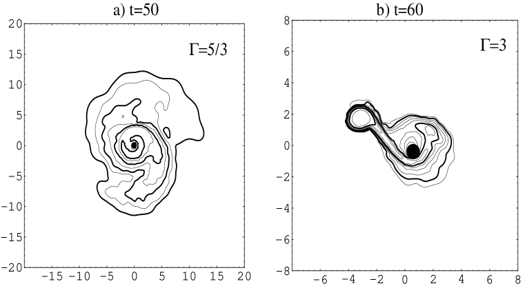
Figure 5: (a) Density contour plots in the orbital plane for run DL1.0 ($\Gamma=5/3$) at $t=50$. All contours are logarithmic and equally spaced every 0.5 dex. Bold contours are plotted at $\log\rho=-5,-4,-3,-2$, in the units defined in section II.2. (b) Same as (a) but for run AL1.0 ($\Gamma=3$) at $t=60$, and with bold contours plotted at $\log\rho=-3,-2,-1$.

By the same arguments as before, the outcome of these coalescence events is reflected in the gravitational radiation signal as an abrupt drop in amplitude (to practically zero) when the star is disrupted (see Figure 4). Again the frequency at which this occurs will give a measure of the radius of the neutron star.

IV Discussion

It is clear that there are serious limitations to the numerical approach we have used to study this type of system, but we nevertheless believe these simulations are useful for many reasons. First, it is clear that hydrodynamical effects can play an important role in the global behavior of the system at small separations, and are crucial to determine the coalescence waveform properly. Second, Newtonian calculations can be used to guide future, more detailed simulations that will incorporate the effects of general relativity, and can serve as useful guides in this respect.

The main result of all our calculations is that the outcome of the coalescence process is very sensitive to the assumed stiffness of the equation of state. For large values of the adiabatic index $\Gamma\simeq 3$ the star is not disrupted, and there is a remnant left in orbit around the black hole, with an accretion disk as well. The gravitational radiation signal exhibits a drop in amplitude and a return to lower frequencies, but does not vanish completely. The coalescence process is delayed for at least several tens of millisconds. For lower values of $\Gamma\simeq 2$, when the star does not alter its radius in response to mass loss (or expands, when $\Gamma<2$), complete tidal disruption is always observed, with massive accretion disks forming around the black hole. The gravitational radiation signal practically vanishes soon after Roche lobe overflow occurs.

In a realistic scenario, the value of $\Gamma$ will not be uniform throughout the star. However, for the purposes of tidal disruption and the gravitational radiation emitted, it is the value at high densities (roughly above nuclear density) that will determine the evolution of the system. We have performed different tests using a variable $\Gamma$ (it is specified as a function of density, examples of this approach can be found in Rosswog et al. 2000), taking a stiff equation of state for high densities, and a softer index for the low density regions. The above discussion concerning tidal disruption is valid in this case as well, if one considers the high–density value of the adiabatic index, and since it is the bulk motion of matter that determines the gravitational wave emission, the value of $\Gamma$ at low densities is unimportant in this respect.

The approach one takes also clearly depends on the problem one wishes to solve. These systems have been suggested as sources for the production of cosmological gamma ray bursts (GRBs) (Paczyński 1986; Goodman 1986; Eichler et al. 1989; Paczyński 1991; Narayan, Paczyński & Piran 1992). Kluźniak & Lee (1998) showed that the conditions during and after coalescence were indeed favorable for this, with the creation of a thick accretion torus and a baryon–free axis in the system, along the rotation axis, that would not hinder the production of a relativistic fireball that could produce a GRB (Mészáros & Rees 1992, 1993). A different equation of state (that of Lattimer & Swesty 1991) has been used by Ruffert & Janka (1996) in the study of double neutron star mergers, and by Janka et al. (1999) in black hole neutron star mergers. The stiffness of this equation of state is not a free parameter, but there is a much greater level of detail in the microphysics, relevant for the implications to GRB models (they additionally included neutrino transport in their calculations). Likewise, regarding the production of heavy elements through r–process nucleosynthesis, a simple ideal gas treatment is inadequate. One must use detailed thermodynamic calcualtions and a realistic equation of state, as Rosswog et al. (1999) and Freiburghaus, Rosswog & Thielemann (1999) have done. Our computations allow us simply to determine how much matter is dynamically ejected from the system during coalescence, a necessary first step if it is to contribute to the observed galactic abundances.

V Acknowledgements

It is a pleasure to thank the organizers for a wonderful workshop. This work was supported in part by CONACyT (27987E) and DGAPA–UNAM (PAPIIT-IN-119998).

References

- (1) Balsara D., 1995, J. Comp. Phys.,121, 357
- (2) Bildsten L., Cutler C., 1992, ApJ, 400, 175
- (3) Davies M.B., Benz W., Piran T., Thielemann F.K., 1994, ApJ, 431, 742
- (4) Eichler D., Livio M., Piran T., Schramm D.N., 1989, Nature, 340, 126
- (5) Freiburghaus C., Rosswog S., Thielemann F.K., 1999, ApJ, 525, L121
- (6) Gingold R.A., Monaghan J.J., 1977, MNRAS, 181, 375
- (7) Goodman J., 1986, ApJ, 308, L46
- (8) Janka H. Th., Eberl T., Ruffert M., Fryer C.L., 1999, ApJ, 527, L39
- (9) Kluźniak W., Lee W.H., 1998, ApJ, 494, L53
- (10) Kochanek C., 1992, ApJ, 398, 234
- (11) Lai D., Rasio F.A., Shapiro S.L., 1993a, ApJ, 406, L63
- (12) Lai D., Rasio F.A., Shapiro S.L., 1993b, ApJS, 88, 205
- (13) Lattimer J.M., Schramm D.N., 1974, ApJ, 192, L145
- (14) Lattimer J.M., Schramm D.N., 1976, ApJ, 210, 549
- (15) Lattimer J.M., Swesty D., 1991, Nuc. Phys. A, 535, 331
- (16) Lee W.H., Kluźniak W., 1995, Acta Astron., 45, 705
- (17) Lee W.H., Kluźniak W., 1999, ApJ, 526, 178 (Paper I)
- (18) Lee W.H., Kluźniak W., 1999, MNRAS, 308, 780 (Paper II)
- (19) Lee W.H., 2000, MNRAS, 318, 606 (Paper III)
- (20) Lucy, 1977, AJ, 82, 1013
- (21) Mészáros P., Rees M., 1992, MNRAS, 257, 29P
- (22) Mészáros P., Rees M., 1993, ApJ, 405, 278
- (23) Monaghan J.J., 1992, ARA& A, 30, 543
- (24) Narayan R., Paczyński B., Piran T., 1992, ApJ, 395, L83
- (25) Paczyński B., 1986, ApJ, 308, L43
- (26) Paczyński B., 1991, Acta Astron., 41, 257
- (27) Rosswog S., Liebendörfer M., Thielemann F.K., Davies M.B., Benz W., Piran T., 1999, A& A, 341, 499
- (28) Rosswog S., Davies M.B., Thielemann F.K., Piran T., 2000, A& A, 360, 171
- (29) Ruffert M., Janka H. Th., 1996, A& A, 311, 532
- (30) Stairs I.H., Arzoumanian Z., Camilo F., Lyne A.G., Nice D.J., Taylor J.H., Thorsett S.E., Wolszczan A., 1998, ApJ, 505, 352
- (31) Symbalisty E.M.D., Schramm D.N., 1982, Astrophyscial Letters, 22, 143
- (32) Zhuge X., Centrella J.M., McMillan S.L.W., 1996, Phys. Rev. D, 54, 7261