Correlation of the South Pole 94 data with $100\mu\mathrm{m}$ and 408 MHz maps

Abstract

We present a correlation between the ACME/SP94 CMB anisotropy data at 25 to 45 GHz with the IRAS/DIRBE data and the Haslam 408 MHz data. We find a marginal correlation between the dust and the Q-band CMB data but none between the CMB data and the Haslam map. While the amplitude of the correlation with the dust is larger than that expected from naive models of dust emission it does not dominate the sky emission.

1 Introduction

The study of Cosmic Microwave Background (CMB) anisotropies has recently proven to be a powerful tool for observational cosmology de Bernardis et al. (2000); Lange et al. (2000); Hanany et al. (2000); Balbi et al. (2000). One of the most important aspects of CMB analyses is to check whether the anisotropies observed are due to CMB temperature fluctuations or to foreground contamination such as diffuse Galactic emission.

Diffuse Galactic emission is dominated at high frequency (above $\approx 100$ GHz) by thermal emission from dust. High quality tracers of this emission are given by the IRAS/DIRBE $100\leavevmode\nobreak\ \mu\mathrm{m}$ maps and have been made available in a user friendly way by Schlegel et al. (1998). At lower frequencies, Galactic emission is dominated by synchrotron and free-free radiation. Our best tracer of the synchrotron emission of the Galaxy is given by the Haslam 408 MHz map Haslam et al. (1981). Free-free emission is traced by H$\alpha$ emission, but maps of this emission are not yet publicly available.

Characterizing the correlations between these different Galactic components and data taken in the microwave is important in order to understand the spectral behaviour and the origin of Galactic emission which may contaminate CMB measurements. The first significant, high-$|b|$ cross-correlation between the COBE/DMR maps and dust templates was found by Kogut et al. (1996a, b). Significant correlations were found at each DMR frequency, but with a spectral behaviour in better agreement with free-free emission than with vibrational dust. These results have been confirmed by different experiments in various parts of the sky: Saskatoon de Oliveira-Costa et al. (1997), OVRO Leitch et al. (1997) and 19 GHz de Oliveira-Costa et al. (1998). At high Galactic latitudes, however, Python V Coble et al. (1999) did not see any correlation. The regions of the sky covered by these experiments are shown in Fig. 1. As noted above, free-free emission should correlate with H$\alpha$ maps. Unfortunately, correlations found between H$\alpha$ maps and the CMB indicate that the H$\alpha$-traced emission is too small to explain all of the observed correlation between CMB data and $100\leavevmode\nobreak\ \mu\mathrm{m}$ data.

Draine and Lazarian (1998a, b) have suggested an alternate explanation for the correlation between CMB data and dust maps, namely that this emission may be the result of rotational dust emission from elongated grains. This emission could be compatible with the observed spectrum of the dust correlated emission in the microwave frequencies.

The sum of dust components, both rotational and vibrational, should show a local minimum at roughly 70 GHz, increase to a peak around 10 GHz, and drop off at lower frequencies. Such behaviour has been observed by de Oliveira-Costa et al. (1999) in correlating the Tenerife 10 and 15 GHz data with the IRAS/DIRBE maps. This has been put forth as evidence supporting spinning dust as the origin of the dust-correlated emission. A recent analysis of yet more Tenerife data Mukherjee et al. (2000) reports, however, that this result should be considered with care, as it originates mainly from a small, high Galactic latitude region. They finally say that the data does not allow any conclusion concerning the origin of the dust correlated emission.

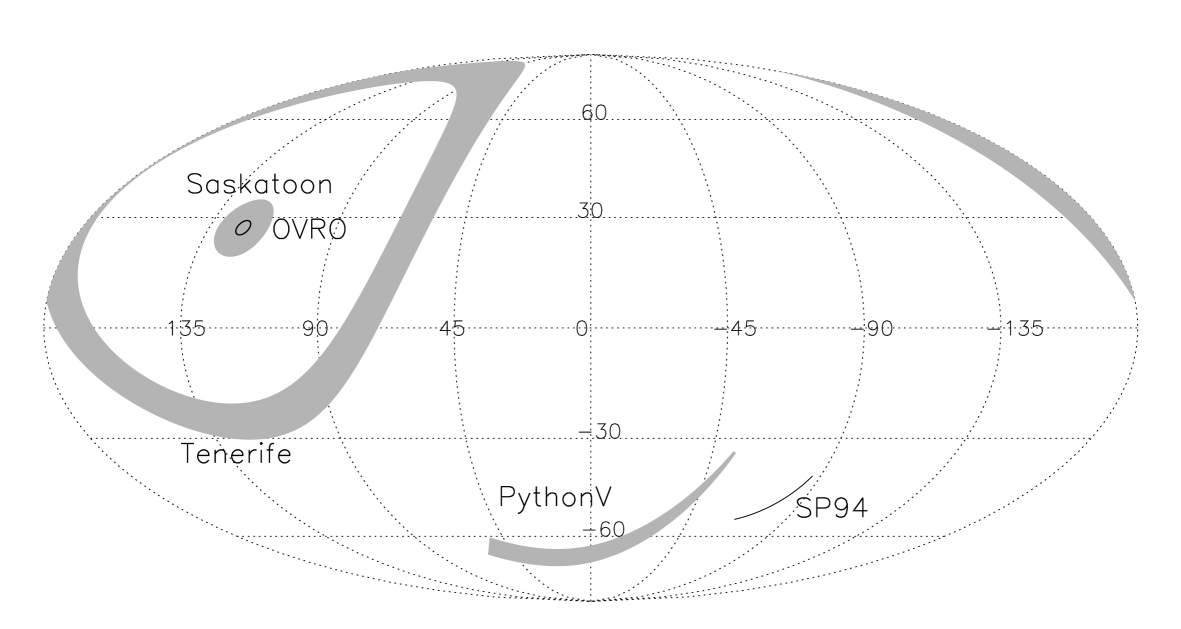
Figure 1: Regions of the sky (in Galactic coordinates) covered by the different experiments that have been correlated with dust. Saskatoon is the grey region around the North Celestial Pole. OVRO observed 36 small patches of the sky at 2 degrees from the Pole. The main part of the Python V coverage is the grey region in the center of the lower part of the map. Tenerife observed a 10 degrees width strip around the North Celestial Pole (grey ring). COBE and 19 GHz both covered the whole sky. South Pole is at the right of Python V.

In this article we present a similar analysis using the South Pole 1994 (SP94) data Gundersen et al. (1995). As correlations in the North Celestial Pole region have recently been questioned, we would like to obtain another measure of the correlation in a different region of the sky. More precisely, as correlations were found at low Galactic latitude (North Celestial Pole) and no correlation was found at high Galactic latitude by Python V, we wanted to explore the correlations in the high latitude regions that will be important for MAP and Planck. SP94 was a CMB experiment that used the Advanced Cosmic Microwave Explorer (ACME) which looked at such a high-$|b|$ region.

2 Data

2.1 Microwave data

The SP94 data were taken in two different bands with 7 different channels: the K_a-band with four center frequencies (27.25, 29.75, 32.25 and 34.75 GHz) and the Q-band with three different frequencies (39.15, 41.45 and 43.75 GHz). A detailed description of the instrument can be found in Meinhold et al. (1993), while the detail of the 1994 observations and data reduction is described in Gundersen et al. (1995). Frequencies and beam width for these channels are given in Table 1.

Channel	Frequency (GHz)	Beam FWHM (deg.)
Ka1	27.25	1.67
Ka2	29.75	1.53
Ka3	32.25	1.41
Ka4	34.75	1.31
Q1	39.15	1.17
Q2	41.45	1.11
Q3	43.75	1.05

Table 1: Frequencies and beam Full-Width-at-Half-Maximum for the different channels.

2.2 Infrared data

In this analysis, we used two templates for each channel :

• For the thermal emission from dust, we used the IRAS/DIRBE map provided by Schlegel et al. (1998). The initial resolution of this map is 6.1 arcmin FWHM.

• For the synchrotron emission, we used the Haslam maps Haslam et al. (1981) whose resolution is 51 arcmin FWHM.

Both maps were convolved to the SP94 beams (for each channel separately) using the beams given in Table 1 and then differenced, simulating the chopping strategy of the SP94 experiment. The simulated signals are shown, along with the SP94 data in Fig. 2. We see from this figure that the correlations, if non-zero, will be rather small.

Figure 2: The top panels shows the coadded SP94 data for the Q-band and for the K_a-band separately. The coaddition was performed using, for each pixel, the full covariance matrix (using the method explained at the end of section 3). The third panel shows the simulated IRAS/DIRBE data (dust) and the bottom panel shows the simulated Haslam data (synchrotron). For both simulated signals, only the 27.25 GHz band is shown, the others are very similar.

3 Method

For each of the seven frequency bands we have $N=43$ data points, all at a declination of $-62^{\circ}$ and ranging from $23^{\circ}$ and $67^{\circ}$ in right ascension (see Fig. 1). These data points were obtained using a sinusoidal $1.5^{\circ}$ chop with smooth, constant declination, constant velocity scans. We directly follow in this section the notation of de Oliveira-Costa et al. (1999). We assume that the data is a linear combination of CMB anisotropies $x^{i}_{CMB}$ and $M$ foreground components (including an unknown offset and gradient) that are given by simulated observations of the template dust and synchrotron maps using the SP94 beam and scanning strategy. In a vector-like notation, one gets :

$${\bf y}=X\@vec{a}+\@vec{x}_{CMB}+\@vec{n}$$ (1)

$X$ is a matrix with $N$ rows and $M$ columns. It contains the template maps observed using the SP94 beams and scanning strategy. $\@vec{a}$ it the $M$-vector we are interested in, it contains the correlation of the SP94 data with the different foregrounds contained in $X$. The experimental noise is $\@vec{n}$.

The noise and the CMB anisotropies are each assumed to be uncorrelated Gaussian variables with zero mean. They each have non-trivial covariance matrices and together a total covariance matrix of:

$$C = \left<\@vec{y}\@vec{y}^{T}\right>-\left<\@vec{y}\right>\left<\@vec{y}^{T}\right>$$ (2)

$$= \left<\@vec{x}_{CMB}\@vec{x}_{CMB}^{T}\right>+\left<\@vec{n}\@vec{n}^{T}\right>=C_{CMB}+C_{n}$$ (3)

As discussed in Gundersen et al. (1995), the noise in a given pixel in given band (K_a or Q) is only correlated with the noise in the same pixel in the different channels of this band (4 channels for the K_a band and 3 channels for the Q band). The noise from the K_a and Q band are uncorrelated.

The covariance matrix of the CMB is obtained through the window function of the South Pole experiment $W_{\ell,ij}^{kl}$ that can be found in Gundersen et al. (1995) :

$$C_{CMB}\leavevmode\nobreak\ {}_{ij}^{kl}=\sum_{\ell=0}^{\infty}\frac{2\ell+1}{4\pi}C_{\ell}W_{\ell,ij}^{kl}$$ (4)

where $\ell$ is the multipole index, $i$ and $j$ denote pixel indices and $k$ and $l$ denote the different channels. The window function was calculated accounting for the different beam-widths for each channel, and the underlying CMB sky was assumed to be the same for all channels. The beam width of each channel can be found in Table 1. $C_{l}$ is the CMB anisotropy angular power spectrum. We used the best fit $\Omega=1$ model from Jaffe et al (2000) obtained with the combined COBE/DMR, BOOMERANG and MAXIMA-1 data sets: $\Omega_{\mathrm{tot}}=1$, $\Omega_{\Lambda}=0.7$, $\Omega_{b}h^{2}=0.03$, $\Omega_{c}h^{2}=0.17$, $n_{s}=0.975$, $\tau_{C}=0$. As a check, we confirmed that the results do not change much using a flat band power spectrum with $Q_{\mathrm{rms-PS}}=20$, $25$ and $30\leavevmode\nobreak\ \mu\mathrm{K}$. The differences were small.

We are interested in measuring the correlation coefficients with the various templates, we therefore want to measure $\@vec{a}$ considering $\@vec{n}$ and $\@vec{x}_{CMB}$ as noise (but accounting for chance alignment between CMB and the templates trough the CMB covariance matrix). We therefore construct the following $\chi^{2}$ :

$$\chi^{2}=\left({\bf y}-X\@vec{a}\right)^{T}C^{-1}\left({\bf y}-X\@vec{a}\right)$$ (5)

Minimising this $\chi^{2}$ leads to the best estimate of $\@vec{a}$ :

$$\hat{\@vec{a}}=\left[X^{T}C^{-1}X\right]^{-1}X^{T}C^{-1}\@vec{y}$$ (6)

We make the fit simultaneously for all channels in order to account for the channel-to-channel correlation matrix elements but the templates (dust and 408 MHz emission) are fitted separately. The vector $\@vec{y}$ contains the concatenated data for all channels ($N$ data points per channel). It is therefore a $(n_{chan}\times N)$ vector. The coadded Q-band and coadded K_a-band data are shown in Fig. 2. The covariance matrix is an $(n_{chan}\times N)\times(n_{chan}\times N)$ matrix. The $X$ matrix contains the template simulated signal (one for each channel) as well as a constant term and a gradient term for each channel, in order to account for the fact that such terms were removed from the SP94 data. The matrix $X$ is therefore a $(n_{chan}\times N)\times(n_{chan}\times 3)$ matrix. In a given column (corresponding to a given channel), $X$ contains mostly zeros, except for the rows corresponding to that channel where it contains the template simulated signal.

The best estimate of $\@vec{a}$ is given through the $\chi^{2}$ minimization along with its covariance matrix:

$$\Sigma=\left[X^{T}C^{-1}X\right]^{-1}$$ (7)

We obtain a correlation coefficient for each channel but those are highly correlated according to the covariance matrix $\Sigma$. The correlation coefficients cannot therefore be averaged in a straightforward manner. We estimate the average of the correlation coefficients via:

$$\chi^{2}=\left(\@vec{a}-\bar{a}\@vec{1}\right)^{T}\Sigma^{-1}\left(\@vec{a}-\bar{a}\@vec{1}\right)$$ (8)

where $\@vec{1}$ is a vector whose elements are all equal to 1. The best estimate of $\bar{a}$ is then obtained by:

$$\bar{a}=\frac{\mathrm{Total}(\Sigma^{-1}\@vec{a})}{\mathrm{Total}(\Sigma^{-1})}$$ (9)

where the $\mathrm{Total}$ function returns the sum of all elements of a matrix or vector. This is equivalent to a weighted average, though in this case we also account for correlations between the different measures. The error-bar on $\bar{a}$ is then:

$$\sigma_{\bar{a}}=\sqrt{\left(\mathrm{Total}(\Sigma^{-1})\right)^{-1}}.$$ (10)

We do this for the K_a- and Q-bands separately, and for the combination of the two. The results are shown in Table 2.

Equations 8,9 and 10 implicitly suppose that the dust-correlated component has a flat spectrum (ie has a spectral index $n=0$). As was mentioned before, results from other experiments tend to favor spectral indices close to $n\simeq-2$ similar to free-free emission. In order to account for a non-zero spectral index, we model the emission as :

$$\bar{a}=\bar{a}_{0}\left(\frac{\nu}{\nu_{0}}\right)^{n}$$ (11)

where $\nu_{0}$ is a reference frequency and not an additional degree of freedom. Equation 8 then becomes :

$$\chi^{2}=\left(\@vec{a}-\bar{a}_{0}\@vec{m}\right)^{T}\Sigma^{-1}\left(\@vec{a}-\bar{a}_{0}\@vec{m}\right)$$ (12)

where $\@vec{m}$ is a vector with 7 elements $m_{i}=\left(\frac{\nu_{i}}{\nu_{0}}\right)^{n}$. This $\chi^{2}$ is not linear if one lets $n$ vary as a free parameter. We therefore minimize it numerically for a grid of 300 values of $n$ between -5 and 5.

4 Correlations

We compute correlations between the SP94 and both dust and synchrotron templates shown in Fig. 2 and Table 2. Those results are also plotted as a function of the frequency in Fig. 3. The results we obtain show a marginal correlation of the Q-band data with the dust IRAS/DIRBE template whereas there is no correlation in the K_a-band. No significant positive correlation is found in either band with the Haslam template. The uncertainty on the combined Q-band and K_a-band correlation coefficients is not as much smaller than that of the Q-band or K_a-band alone as one might naively expect. In fact, this is due to the contribution of the CMB covariance matrix. For each channel, the CMB covariance matrix is comparable to the noise one and therefore combining the data reduces the noise contribution but not the CMB one that becomes dominant.

In Table 2, we also show the result for the analysis allowing the spectral index to vary as a free parameter. Combining the K_a channels did not lead to any realistic value for the spectral index (the best fit, $n=5.0$, was at the edge of the range we searched). Combining the Q-band data leads to a best fit for the spectral index of $n=0.8\pm 2.0$. Combining all K_a and Q data together leads to $n=2.1\pm 1.0$. It is there clear that positive values are preferred. This is not a surprise, however, as the Q-band data obviously correlate with the IRAS data better than the K_a does.

Figure 3: Correlations coefficients between the SP94 data and the templates (top: with IRAS/DIRBE and bottom: with Haslam 408 MHz). The combined correlation coefficient assume a spectral index $n=0$ for the correlated component.

We summarize in Fig. 4 the measurements performed up to now of the correlation with the vibrational dust traced by IRAS/DIRBE $100\mu\mathrm{m}$ : SP94 corresponds to the present article, the Tenerife measurements have been published in two different articles de Oliveira-Costa et al. (1999); Mukherjee et al. (2000) reporting slightly different results obtained with almost the same data. We plot both measurements, the lower values were obtained by de Oliveira-Costa et al. (1999) and considered as a possible evidence for the presence of spinning dust because of the fall at 10 GHz. The upper measurements Mukherjee et al. (2000) were published more recently and mitigated the enthusiasm for spinning dust. As the values in this region are under question now, we plotted a square around these points. OVRO measured one point in this region at 14.5 GHz Leitch et al. (1997) that seems to favour upper values of the correlation. Saskatoon data are taken from de Oliveira-Costa et al. (1997) and show a $1\sigma$ detection in the K_a-band (not significant) and a $1.9\sigma$ detection in the Q-band. The 19 GHz (whole sky survey) data were taken from de Oliveira-Costa et al. (1998). The result from PythonV at 41 GHz was taken from Coble et al. (1999) and is fully compatible with no detection (the best fit is negative and does not appear in the plot). The COBE data points are from Kogut et al. (1996b). The results quoted in the article were obtained by fitting DIRBE $140\mu\mathrm{m}$ to the DMR data. We therefore corrected them by the average ratio DIRBE $140\mu\mathrm{m}$/DIRBE $100\mu\mathrm{m}$ to have them in the same units as the other data points. The FIRS point at 167 GHz was obtained by Ganga (1994). We also overplotted in Fig. 4 the predicted spectrum (in terms of ratio to IRAS/DIRBE $100\mu\mathrm{m}$) for vibrational dust in green (we assumed a spectral index of $2.0$) normalised with IRAS/DIRBE $100\mu\mathrm{m}$, and for spinning dust in blue. We also added the spectrum for free-free emission in light blue (arbitrary normalization and spectral index -2.1). For the spinning dust, we follow Draine and Lazarian (1998a) for the mixing between Warm Ionised Medium (WIM), Warm Neutral Medium (WNM) and Cold Neutral Medium (CNM) models using a respective fraction of 0.14, 0.43 and 0.43. The respective normalization of these models was also taken from Draine and Lazarian (1998a). The sum of both contributions is shown in Fig. 4 in red. The width of the curves for the spinning dust model is due to the galactic latitude dependance of the optical depth of the spinning dust components. We used all the latitudes more than $20^{\circ}$ from the Galactic equator. The normalization is that given by Draine and Lazarian (1998a). As clearly yields too little emission to match the data, we have also done a fit to the points and arbitrarily raised the model curves by this amount. This is indicated by the dotted curve.

Band	$n$	100 $\mu$m	sig.	408 MHz	sig.
Ka1	-	$-0.8\pm 38.4$	$-0.0$	$7.4\pm 16.5$	$0.4$
Ka2	-	$48.4\pm 39.4$	$1.2$	$-4.8\pm 16.3$	$-0.3$
Ka3	-	$13.9\pm 40.5$	$0.3$	$-9.9\pm 16.1$	$-0.6$
Ka4	-	$69.1\pm 41.5$	$1.7$	$-17.6\pm 16.0$	$-1.1$
Ka	-2.0	$-16.6\pm 20.2$	$-0.8$	-	-
Ka	0.0	$20.7\pm 36.8$	$0.6$	$-8.0\pm 15.1$	$-0.5$
Ka	0.8	$49.2\pm 40.9$	$1.2$	-	-
Ka	2.0	$78.0\pm 50.0$	$1.9$	-	-
Ka	2.1	$79.4\pm 40.7$	$2.0$	-	-
Q1	-	$58.3\pm 46.0$	$1.3$	$-15.9\pm 16.9$	$-0.9$
Q2	-	$71.8\pm 43.2$	$1.7$	$-20.3\pm 15.5$	$-1.3$
Q3	-	$66.9\pm 44.0$	$1.5$	$-14.9\pm 15.5$	$-1.0$
Q	-2.0	$73.5\pm 54.2$	$1.4$	-	-
Q	0.0	$68.1\pm 42.5$	$1.6$	$-17.5\pm 15.2$	$-1.2$
Q	0.8	60.1 $\pm$ 37.0	1.6	-	-
Q	2.0	$44.4\pm 28.2$	$1.6$	-	-
Q	2.1	$42.8\pm 27.3$	$1.6$	-	-
All	-2.0	$-25.3\pm 20.2$	$-1.4$	-	-
All	0.0	$22.2\pm 36.8$	$0.6$	$-12.4\pm 14.6$	$-0.9$
All	0.8	$63.5\pm 36.7$	$1.7$	-	-
All	2.0	$56.8\pm 24.8$	$2.3$	-	-
All	2.1	54.2 $\pm$ 23.6	2.3	-	-

Table 2: Correlations coefficients between the SP94 data and the templates : We also give the coadded correlation coefficients found by combining the K_a channels, the Q band channels and for all channels together. The second column gives the assumed correlated signal spectral index in each case (we considered $n\neq 0$ only for the correlation with dust). The third column shows the coefficient of the correlation with the dust IRAS/DIRBE simulated signal (in $\mu\mathrm{K}.(\mathrm{MJy/sr})^{-1}$) for each spectral index and the fifth column shows this correlation for the Haslam 408 MHz simulated signal (in $\mu\mathrm{K}.K^{-1}$). The fourth and sixth columns indicate the significance in terms of number of sigma of the correlation measured. No best fit was found in the range $-5\leq n\leq 5$ for the combined K_a channels. For the combined $Q$ channels, the best fit was found for $n=0.8$ and is shown in bold. Combining all the channels leads to a best fit at $n=2.1$ also shown in bold.

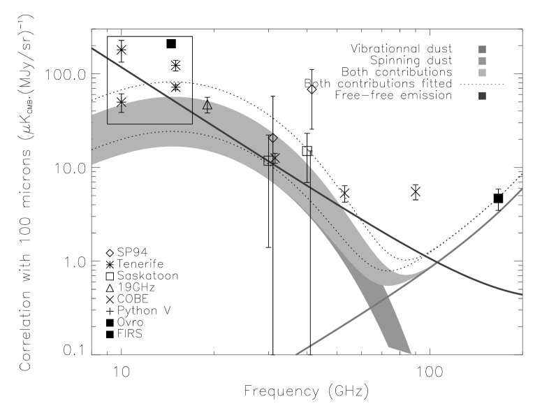
Figure 4: CMB/IRAS correlation coefficients as measured by various experiments. We overplot the spectra for vibrationnal dust, spinning dust and the sum of the two. The vibrationnal dust spectrum assumes a spectral index of 2.0 and was normalized to match averages of DIRBE at Galactic latitudes higher than 20 degrees. The spinning contribution is normalized following (Draine and Lazarian, 1998a). To guide the eye, we also plot the best fit of the models to the dta in dotted lines. We also added a free-free emission spectrum with a spectral index of -2.1 and an arbitrary normalization.

5 Discussion and conclusion

The signal to noise for the Q-band detection is only 1.6 ($89\%$ confidence level) so this would not be considered a detection as most CMB experiments require at least 2$\sigma$. We would note however that, as opposed to normal CMB anisotropy analyses, here we are comparing the data to a template and it is difficult to imagine that systematic effects or analysis errors that would cause a random correlation with $100\mu\mathrm{m}$ dust emission. The correlation could arise from random alignment between the CMB anisotropies and the dust template. This, however, should be taken into account in our analysis if our covariance matrices for the data and the CMB are correctly estimated. If these covariance matrices were underestimated, the error bars we compute on the correlation coefficient (with Eq. 7) would be too small and therefore the significance of our result would be overestimated. In order to check the validity of our error bars, we correlated the SP94 data with template dust maps obtained by rotating the initial template maps around the Galactic poles and by inverting North and South. The Galaxy was either rotated and/or inverted in 36 different ways (10 degrees each) to make 36 different simulations. We found a zero average correlation and the RMS of the correlations normalized by the error bars (calculated with Eq. 7) appears to be 1.1. This shows that the covariance matrices of the CMB and the data and therefore our error bars are correctly estimated, confirming the significance of the correlation coefficients we obtain.

We do, however, find the following points interesting: As seen previously de Oliveira-Costa et al. (1997) the correlation between the Q-band and the $100\mu\mathrm{m}$ emission is stronger than the correlation between the K_a-band and the $100\mu\mathrm{m}$ emission. If the correlation we found is to be believed, the ratio of the RMS of the $100\mu\mathrm{m}$ template times the fitted correlation coefficient to the implied sky RMS is $0.38$ (in the Q-band). This result indicates that roughly $14\%$ of the power seen on the sky by ACME/SP94 Q-band could be due to Galactic emission. The $C_{\ell}$ could go down by $14\%$ and the amplitude by $38\%$. This however does not apply to the K_a-band. This result is in qualitative agreement with Gundersen et al. (1995) and Ganga et al. (1997), both of which found different spectral indices for the K_a- and Q-band data, though again, with low statistical significance.

We have also done the above analysis using as a template not the raw $100\mu\mathrm{m}$ data but rather the extrapolations recommended by Schlegel et al. (1998) (model 8) to 500GHz and 40 GHz. The $\chi^{2}$ for the fit went down by a very small amount. The differences in the $\chi^{2}$ were not significant and do not change the conclusions drawn above. This is not surprising as the SP94 data covers only a small region and the SFD model was designed to cope with the whole sky.

In conclusion, we have shown that there is a very marginal correlation between the SP94 Q-band data and vibrational dust tracers, while no such correlation exists with the 408 MHz map. The amplitude of the correlation in the Q-band is larger than that seen by de Oliveira-Costa et al. (1997).