*

Abstract

Gravitational weak shear produced by large-scale structures of the universe induces a correlated ellipticity distribution of distant galaxies. The amplitude and evolution with angular scale of the signal depend on cosmological models and can be inverted in order to constrain the power spectrum and the cosmological parameters. We present our recent analysis of 50 uncorrelated VLT fields and the very first constrains on ($\Omega_{m},\sigma_{8}$) and the nature of primordial fluctuations based on the join analysis of present-day cosmic shear surveys.

1 Motivations

The deformation of light beams produced by gravitational tidal fields is responsible for the cosmological weak lensing signal (or cosmic shear) produced by large-scale structures of the universe. The statistical properties of the gravity-induced convergence, $\kappa$ (the projected mass density) and shear, $\gamma$ (the distortion) primarily depend on the normalization of the power spectrum of mass density fluctuations, $\sigma_{8}$, and on the density parameters, $\Omega_{m}$, and can be used to constrain cosmological scenarios. Bernardeau et al [1] showed that the sensitivity of cosmological models to these quantities is well described by the variance and the skewness of $\kappa$ averaged over the angular scale $\theta$, $\langle\kappa(\theta)^{2}\rangle^{1/2}$ and $s_{3}(\theta)$

$$\langle\kappa(\theta)^{2}\rangle^{1/2}\approx\ 0.01\ \sigma_{8}\ \Omega_{m}^{\ 0.75}\ z_{s}^{\ 0.8}\left({\theta\over 1^{o}}\right)^{-(n+2)/3}\ ,$$ (1)

$$s_{3}(\theta)\approx\ 40\ \Omega_{m}^{\ -0.8}\ z_{s}^{\ -1.35}\ {}^{\prime}$$ (2)

where $z_{s}$ is the redshift of sources. Hence, a cosmic shear survey which would focus on the measurement of the variance and the skewness of $\kappa$ should recover both $\Omega_{m}$ and $\sigma_{8}$ independently.
Although the gravitational convergence is very weak, on angular scales smaller than 10 arc-minutes it is enhanced by the the non-linear gravitational structures, which increase the lensing signal by a significant amount (see Jain & Seljak 1997, [2]). On those scales, the cosmological weak lensing can already be measured from the gravity-induced ellipticity of galaxies (the shear) even with ground-based telescopes. In fact, as it is shown by van Waerbeke et al 1999 ([3]) and in Table 1, one needs to cover about one deg² up to $I\approx 24.5$ in order to measure cosmic shear on small scales.
Four teams recently presented first results. The most recent work was performed by Maoli et al 2000 ([4]) using VLT/FORS1 and has been used jointly with other surveys to explore cosmological models. This work is summarized below.

Table 1: Expected signal-to-noise ratio on the the variance and the skewness of the convergence for two cosmological models. In the first column, the size of the field of view (FOV) is given. The signal-to-noise ratio is computed from the simulations done by van Waerbeke et al (1999).

$z_{s}=1$, Top Hat Filter , $n=30$ gal.arcmin-2
FOV	S/N Variance		S/N Skewness
(deg.$\times$deg.)	$\Omega_{m}=1$	$\Omega_{m}=0.3$	$\Omega_{m}=1$	$\Omega_{m}=0.3$
1.25$\times$1.25	7	5	1.7	2
2.5$\times$2.5	11	10	2.9	4
5$\times$5	20	20	5	8
10$\times$10	35	42	8	17

2 Description of the VLT survey

The VLT sample is defined in order to get a large number of fields separated from each other by an angular distance as large as possible. This criterion enables us to minimize the cosmic variance. The selection of the field sample is optimized as follows:

• no stars brighter than 8th magnitude inside a circle of 1 degree around the FORS field, and no stars brighter than 14th magnitude inside the FORS field, in order to avoid light scattering;

• no extended bright galaxies in the field. Their extended halo may contaminate the shape of galaxies located nearby;

• neither rejection of over-dense regions, where clusters or groups of galaxies could be present, nor primarily selection towards empty fields. Otherwise, the sample could be biased toward under-dense regions with systematically low value of the convergence;

• angular separation between each pointing larger than 5 degrees in order to minimize the correlation between fields;

• field must be galactic latitudes lower than $70^{\circ}$ in order to get enough stars per field for the PSF correction.

We selected 50 FORS1 fields, each covering 6.8’$\times$6.8’. The total field of view is 0.64 deg² and the pointings are randomly spread over more than 1000 deg². So far, this is the largest sample of uncorrelated fields used for cosmic shear analysis.
The observations were obtained with FORS1 on the VLT/UT1 (ANTU) at the Paranal Observatory in I-band only. They were carried out in service mode which turns out to be perfectly suited for our program. All the exposures have a seeing between 0.55” and 0.80” with a median value at 0.64”. The total exposure time per field is 36 minutes. It has been computed in order to reach $I=24.5$, which corresponds to a galaxy number density per fields of about 30$\pm$ 10 gal.${\rm arcmin}^{-2}$. At this depth, the expected average redshift of the lensed sources is $\langle z\rangle\approx 1$. Note that thanks to the service mode observation, the VLT sample provides the most homogeneous sample we have. From this sample, we extracted 76,000 galaxies. Due to the severe selection criteria used for cosmic shear, the final sample only has 50,000 galaxies.

3 Results of cosmic shear experiments

So far, four teams have completed a cosmic shear survey. Each of them observed different fields of view and used different instruments and techniques to get and to analyze the data (see Table 2). The CFHT and VLT surveys reported in van Waerbeke et al [5] and Maoli et al [4] respectively consist in two independent data sets. We used them also to cross-check our results and to explore the reliability of our corrections of systematics. The VLT sample complements our CFHT data which has the same depth, covers a much larger area ( 1.7 deg²) but only contains 5 uncorrelated fields. The use of both set of data simultaneously represents 75% of the total number of fields and 40% of the total area covered by all cosmic shear surveys.
A description of the five surveys is summarized in Table 2 and the results are in Fig. 1. The most striking feature on this plot is the remarkable similarity of the results in the range 1’ to 10’ . This is a very strong point which validates the detection and guarantees that they are reliable and robust, despite concerns about systematics.

Table 2: Summary of the 5 cosmic shear surveys completed so far. The CFHT data were obtained with the UH8K and CFH12K CCD cameras. The R and I limiting magnitudes enables us to estimate of the redshift of the sources, which should be around one.

Reference	Telescope	Lim. Mag.	FOV	Nb. fields
van Waerbeke et al [5]	CFHT	I=24	1.7 deg2	5
Wittman et al [6]	CTIO	R=26	1.5 deg2	3
Bacon et al [7]	WHT	R=24	0.5 deg2	13
Kaiser et al [8]	CFHT	I=24	1.0 deg2	6
Maoli et al [4]	VLT-UT1	I=24	0.5 deg2	45

Figure 1: $\left<\gamma^{2}\right>$ as function of the angular scale ($\theta$ is the angular diameter of a circular top-hat). The filled squares are the VLT data. The other detection are [5] (vWME+), [7] (BRE), [6] (WTK) and [4] (KWL). They are compared to current cosmological models assuming a standard galaxies redshift distribution with $z_{0}=0.8$. For all models we choose a CDM power spectrum with $\Gamma=0.21$, and $\Omega_{0}=1$, $\Lambda=0$, $\sigma_{8}=1$ (short dash); $\Omega_{0}=0.3$, $\Lambda=0$, $\sigma_{8}=1.02$ (dot long-dash); $\Omega_{0}=1.0$, $\Lambda=0$, $\sigma_{8}=0.6$ (dot) and $\Omega_{0}=0.3$, $\Lambda=0.7$, $\sigma_{8}=1.02$ (solid). The models have been computed using the non-linear evolution of the power spectrum given by [9].

4 Cosmological interpretation of cosmic shear signal

The results plotted in Figure 1 confirm that the Standard CDM predictions are incompatible with most observations, including cosmic shear. In contrast, cosmic shear predictions of most realistic cluster normalized models are all satisfactory, at least on scales ranging from 0.5 to 10 arc-minutes. It is therefore interesting to explore more thoroughly a large set of models in a ($\Omega_{0}$,$\sigma_{8}$) space by using the five cosmic shear results simultaneously. The full sample contains 75 uncorrelated fields and covers 5.5 deg.², so it can already provide reliable informations.
Since the five samples are independent, each provides one single measurement point to perform a simple $\chi^{2}$ minimization in the ($\Omega_{0}$,$\sigma_{8}$) plane. From each sample we choose only one point corresponding to the angular scale where the signal has the best signal-to-noise, taking care to discard the large scale measures, as they are likely affected by finite size effects (see Szapudi & Colombi 1996,[10]). We extracted five triplets containing the scale, the variance and the 1-$\sigma$ error, ($\theta_{i}$, $\gamma^{2}(\theta_{i})$,$\delta\gamma^{2}(\theta_{i})$) reported on Figure 1) and computed:

$$\chi^{2}={\displaystyle\sum_{i=1}^{5}\left[{\gamma^{2}(\theta_{i})-\langle\gamma^{2}\rangle_{\theta_{i}}\over\delta\gamma^{2}(\theta_{i})}\right]^{2}},$$ (3)

where $\langle\gamma^{2}\rangle_{\theta_{i}}$ is the predicted variance for a given cosmological model. We computed it for 150 models inside the box $0<\Omega_{0}<1$ and $0.2<\sigma_{8}<1.4$, with $\Gamma=0.21$, $\Lambda=0$, and $z_{0}=0.8$. The result is given in Figure 2. The grey scales indicates the 1, 2 and 3-$\sigma$ confidence level contours. We fitted the best models by the empirical law:

$$\sigma_{8}\simeq 0.59^{+0.03}_{-0.03}\ \Omega_{0}^{-0.47}$$ (4)

in the range $0.5<\theta<5$ arc-minutes which is found to be is in good agreement with [2] who predicted $\sigma_{8}\propto\Omega_{0}^{-0.5}$ at non-linear scales. Moreover, this is very close to the cluster normalization constraints given in [11] (for closed models and $\Gamma=0.23$):

$$\sigma_{8}\simeq 0.495^{+0.034}_{-0.037}\ \Omega_{0}^{-0.60}\$$ (5)

although the two methods are totally independent. The interpretation of the remarkable agreement between the cluster abundance and the cosmic shear analysis may be the following. The empirical law found from cluster abundance closely follows theoretical expectation of a Gaussian initial density fluctuations field (White et al 1993, [12]). Since the amplitude of cosmic shear signal on scales smaller than 10 arc-minutes mainly probes non-linear mass density contrast like groups and clusters, the similarity between both empirical laws strengthens the assumptions that mass density fluctuations grew from a Gaussian field.
Although encouraging, our interpretation of cosmic shear results depends on critical shortcomings. We only have five independent data points spread over a rather small angular scale and we do not have serious estimates on the redshift of the sources. Assuming they are at $z_{0}=0.8$ is a reasonable assumption ([13]), but it is still uncertain and needs further confirmations. We also neglected the cosmic variance in the error budget of the cosmic shear sample. It does not affect the VLT data which contain 50 uncorrelated fields and, likely, the Bacon et al ([7]) observations (because they estimated the cosmic variance using a Gaussian field hypothesis). The three other measures are probably more affected, although numerical simulations indicate that cosmic variance should only increase our error bars by less than a factor of two (see [5]).

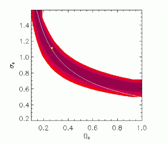
Figure 2: The $\Omega_{0}$-$\sigma_{8}$ constraint derived from combined cosmic shear surveys. The three grey areas define the 1, 2 and 3-$\sigma$ limits. The cross indicates the position of the best fit at $\Omega_{0}=0.26$ and $\sigma_{8}=1.1$. The solid line shows the local cluster abundance best fit ([11]). The latter and the cosmic shear constraints have similar shape and match very well.

5 Conclusions

Although cosmic shear surveys started less than two years ago, they went incredibly fast to provide consistent measurements on small scales. The study discussed in this proceeding goes even further. It both shows the important immediate potential of cosmic shear for cosmology and the fact that FORS1 in service mode is one of the best instrument for this project. It enables to get a homogeneous data set on a very large sample of uncorrelated fields.
On Figure 3, we have simulated the amount of data one would need in order to increase the signal-to-noise ratio by a factor of 3. It turns out that with 300 FORS1 fields obtained in service mode (that is, 250 more fields than what we got, or 160 hours of ANTU/FORS1 in service mode) the separation between most popular model would be striking. If the VMOS instrument (Le Fèvre et al 2000, [14]) provides similar image quality, one can imagine even more impressive results up to angular scales of 15 arc-minutes. The join use of both CFHT and VLT data would therefore be spectacular. In particular, the skewness of the convergence, which is insensitive to $\sigma_{8}$, will appear as a very narrow vertical constraint on Figure 2 therefore breaking the $\Omega_{0}$-$\sigma_{8}$ degeneracy.

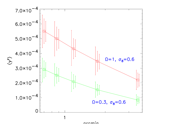
Figure 3: Illustration of the signal-to-noise of the variance of the shear for 100, 150 and 300 VLT/FORS1 fields. One can see that for 300 hundred fields, the two models will be disentangled with a 3$\sigma$ confidence level.

References

- [1] Bernardeau, F., van Waerbeke, L., Mellier, Y. 1997, A&A 322, 1.
- [2] Jain, B., Seljak, U. 1997, ApJ 484, 560.
- [3] van WaerbeKe, L., Bernardeau, F., Mellier, Y. 1999, A&A 342, 15.
- [4] Maoli, R., Mellier, Y., Van Waerbeke, L. et al 2000, A&A in press. Astro-ph/0011251.
- [5] van Waerbeke, L., Mellier, Y., Erben, T. et al 2000, A&A 358, 30.
- [6] Wittman, D.M., Tyson, A.J.,, Kirkman, D. et al 2000, Nature 405, 143.
- [7] Bacon, D., Réfrégier, A., Ellis, R.S. 2000, MNRAS 318, 625.
- [8] Kaiser, N., Wilson, G., Luppino, G. 2000, Astro-ph/0003338.
- [9] Peacock, J. A., Dodds, S. J. 1996, MNRAS 280, 19.
- [10] Szapudi, I., Colombi, S., 1996, ApJ, 470, 131.
- [11] Pierpaoli, E., Scott, D., White, M., 2000. Preprint astro-ph/0010039.
- [12] White, S.D.M., Efstathiou, G., Frenk, C.S., 1993, MNRAS 262, 1023.
- [13] Cohen, J. G., Hogg, D. W., Blandford, R. D., Cowie, L. L., Hu, E., Songaila, A., Shopbell, P., Richberg, K., 2000, ApJ 538, 29.
- [14] Le Fèvre, O., et al. 2000. Proceedings of the ESO conference “Deep Fields”. Arnouts S. et al. eds.