Spitzer View of Young Massive Stars in the LMC H II Complex N 44

Abstract

The H II complex N 44 in the Large Magellanic Cloud (LMC) provides an excellent site to perform a detailed study of star formation in a mild starburst, as it hosts three regions of star formation at different evolutionary stages and it is not as complicated and confusing as the 30 Doradus giant H II region. We have obtained Spitzer Space Telescope observations and complementary ground-based 4m $uBVIJK$ observations of N 44 to identify candidate massive young stellar objects (YSOs). We further classify the YSOs into Types I, II, and III, according to their spectral energy distributions (SEDs). In our sample of 60 YSO candidates, $\sim 65$% of them are resolved into multiple components or extended sources in high-resolution ground-based images. We have modeled the SEDs of 36 YSOs that appear single or dominant within a group. We find good fits for Types I and I/II YSOs, but Types II and II/III YSOs show deviations between their observed SEDs and models that do not include PAH emission. We have also found that some Type III YSOs have central holes in their disk components. YSO counterparts are found in four ultracompact H II regions and their stellar masses determined from SED model fits agree well with those estimated from the ionization requirements of the H II regions. The distribution of YSOs is compared with those of the underlying stellar population and interstellar gas conditions to illustrate a correlation between the current formation of O-type stars and previous formation of massive stars. Evidence of triggered star formation is also presented.

1 Introduction

Star formation frequently takes place in high concentrations of massive stars at intense levels, a phenomenon referred to as “starbursts.” The massive stars in a starburst can inject energies into the interstellar medium (ISM) to photoionize the ambient medium and to dynamically sweep up the medium into expanding shells. The expanding shells can trigger subsequent star formation either by compressing ambient dense clouds or by collect-and-collapse within the shell (Elmegreen, 1998). Starbursts can easily spread over areas 10²-10³ pc across, and play a vital role in determining the large-scale structures of their host galaxies.

While starbursts are the most prominent features in a galaxy, their detailed properties cannot be easily studied: in distant galaxies the stellar content is not resolved and in the Milky Way the distances and association among stars in a starburst are uncertain. The Large and Small Magellanic Clouds (LMC & SMC; MCs) are the only galaxies in which stars are at common, known distances and can be individually resolved down to $\sim$1 $M_{\odot}$ at optical wavelengths (Gouliermis et al., 2006; Nota et al., 2006). Recent Spitzer Space Telescope observations in the mid-infrared (mid-IR) enabled the detection of individual young stellar objects (YSOs) in the MCs, revealing the on-going star formation (Chu et al., 2005; Jones et al., 2005; Caulet et al., 2008). It is now possible to use the resolved stellar population to map out star formation as a function of space and time in the MCs. As the ISM of the MCs has been surveyed in great detail, it is further possible to determine the relationship between star formation and the physical properties of the ISM. Consequently, studies of starbursts in the MCs allow us to investigate fundamental issues about star formation, such as whether and how the stellar energy feedback from massive stars triggers the formation of next-generation stars, whether the initial mass function (IMF) depends on the interstellar conditions for star formation, and whether massive stars are formed only under specific conditions (Zinnecker & Yorke, 2007).

We have chosen the H II complex LH$\alpha$ 120-N 44 (N 44; Henize, 1956) in the LMC to carry out a comprehensive study of star formation in a mild starburst situation, as it is one of the top ranking H II complexes in the LMC but is not as complicated and confusing as the giant H II region 30 Doradus. N 44 contains three OB associations, LH47, 48, and 49 (Lucke & Hodge, 1970), that are in different evolutionary stages and interstellar structures: LH47 in the central superbubble, LH48 in one contiguous H II region at the northeast rim of the superbubble, and LH49 in a group of H II regions to the southeast exterior of the superbubble (Figures. 1a,b). Along the western rim of the superbubble exist a number of dense H II regions where star formation may have been triggered by the expansion of the superbubble (Oey & Massey, 1995). Surveys of CO in the N 44 complex (Fig. 1d; Fukui et al., 2001) show a high concentration of molecular gas at the western rim of the central superbubble, another high concentration at the H II regions around LH49, and a weaker concentration to the north of the superbubble where a couple of small H II regions are visible but no OB associations are identified.

The effects of stellar energy feedback are evident in N 44. The H$\alpha$ image (Fig. 1a) shows the reach of stellar UV radiation. The X-ray image (Fig. 1c) reveals 10⁶ K gas heated by fast stellar winds and supernova explosions. While the expansion of the central superbubble may have triggered the intense star formation along its western rim, the hot gas outflow from the superbubble may be responsible for the onset of star formation at the northeastern extension of the south molecular peak.

To study the current star formation in N 44, we have obtained Spitzer mid-IR and complementary ground-based optical and near-IR observations. These observations have been analyzed and the results are reported in this paper. Section 2 describes the observations and data reduction. Section 3 reports the initial identification of YSO candidates and Section 4 describes a further pruning of the YSO candidate list. In Section 5 we classify the YSOs, and in Section 6 we determine their physical properties by modeling their spectral shapes. In Section 7 we discuss the massive star formation properties. A summary is given in Section 8.

2 Observations and Data Reduction

We have obtained Spitzer mid-IR observations to diagnose YSOs. To extend the spectral energy distribution (SED) and to improve the angular resolution, we have further obtained ground-based optical and near-IR imaging observations of N 44. We have also retrieved available images in the Hubble Space Telescope (HST) archive to examine the optical counterparts and environments of the YSOs.

2.1 Spitzer IRAC and MIPS Observations

Our Spitzer observations of N 44 were made with the InfraRed Array Camera (IRAC; Fazio et al., 2004) on 2005 March 27 and the Multiband Imaging Photometer for Spitzer (MIPS; Rieke et al., 2004) on 2005 April 7. The IRAC observations were obtained in the 3.6, 4.5, 5.8, and 8.0 $\mu$m bands using the mapping mode to cover a $\sim 30^{\prime}\times 30^{\prime}$ area in each band. The pixel size was 1$\farcs$2 pixel^-1, and the common area covered by all four bands is $\sim 30^{\prime}\times 23^{\prime}$. At each pointing, exposures were made with a five-point cyclic dithering pattern in the 30 s high dynamic range mode. The total integration time at each pointing is $\sim$ 150 s. The mosaicked maps were processed with the Spitzer Science Center (SSC) pipeline (ver. S11.4.0) and provided to us as part of the Post Basic Calibrated Data (PBCD) products.

The MIPS observations were made in the 24, 70, and 160 $\mu$m bands using the scan map mode at the medium scan rate. The mapping consists of sixteen $0\fdg 5$ scan legs with a cross-scan step of 148^′′ to cover a region of $20^{\prime}\times 30^{\prime}$ in all three MIPS bands. The MIPS DAT version 3.00 (Gordon et al., 2005) was used for the basic processing and final mosaicking of the individual images. In addition, the 24 $\mu$m image has been corrected for a readout offset and divided by a scan-mirror-independent flat field, and the 70 and 160 $\mu$m images have been corrected for a pixel-dependent background using a low-order polynomial fit to the source-free regions. The final mosaicked maps have pixel scales of 1$\farcs$25, 9$\farcs$85, and 16$\farcs$0 pixel^-1, and exposure times of roughly 160, 80, and 16 s at 24, 70, and 160 $\mu$m, respectively.

The common area covered by all IRAC and MIPS bands is $20^{\prime}\times 23^{\prime}$. To achieve a more complete view of the molecular cloud to the north of N 44 superbubble, we have used the Spitzer survey of the LMC (SAGE, Meixner et al., 2006) to extend our IRAC 3.6 and 5.8 $\mu$m data in the declination direction. The final IRAC and MIPS field we have analyzed is $20^{\prime}\times 25^{\prime}$.

To carry out aperture photometry for point sources in the IRAC images we use the IRAF package apphot. First, the sources were identified with the automated source finding routine daofind, using parameters optimized to find the majority of point-like sources while minimizing the inclusion of peaks of extended dust emission. In regions containing multiple sources superposed on extended emission, daofind does not always identify the same sources at the same locations in the four IRAC bands. Therefore, we identified sources in each of the four IRAC bands and merged the four source lists into a master source list using 1$\farcs$2 (= 1 pixel) as the criterion for coincidence. The resulting master list is then used for photometric measurements in all four bands. The photometric measurements were made with a source aperture of 3$\farcs$6 (3-pixels) radius and an annular background aperture at radii of 3$\farcs$6–8$\farcs$4 (3–7 pixels). Finally, an aperture correction was applied, and the fluxes were converted into magnitudes using the correction factors and zero-magnitude fluxes provided in the IRAC Data Handbook and listed in Table 1.

The photometric measurements from long- and short-exposure IRAC observations were averaged with weights proportional to the inverse square of their errors. For sources that were saturated in the long exposures, their measurements from the short exposures were adopted. The results were used to produce a photometric catalog of 17,002 IRAC sources in the $20^{\prime}\times 25^{\prime}$ field of N 44. This catalog is presented as an ASCII table and an example is shown in Table 2.

MIPS images have lower angular resolution. Source identification using daofind is feasible only for the 24 $\mu$m images. In the 70 and 160 $\mu$m images, point sources cannot be easily resolved from one another or from a bright diffuse background; therefore, the few apparent point sources were identified by visual inspection. The photometric measurements were made with parameters appropriate for the point spread functions (PSFs), as recommended in the MIPS Data Handbook and given in Table 1. Note that the aperture corrections adopted for 70 and 160 $\mu$m measurements are those for sources of temperatures 15 and 10 K, respectively. For sources of higher temperatures, such as 1000–3000 K, the adopted aperture corrections will result in fluxes 8% too high in 70 $\mu$m and 2% too high in 160 $\mu$m because the source emission peaks at shorter wavelengths; however, these errors do not significantly affect the analysis and conclusions of our study of YSOs. In the 160 $\mu$m image, only one point source can be clearly identified; therefore, the 160 $\mu$m photometry will be discussed in the text but not included in the photometric catalog. The catalogs of the MIPS 24 and 70 $\mu$m bands are merged with the IRAC catalog and included in Table 2.

The Spitzer images of N 44 in the 3.6, 8.0, and 24 $\mu$m bands are shown in Figure 2. The 3.6 $\mu$m image is dominated by stellar emission, the 8.0 $\mu$m image shows the polycyclic aromatic hydrocarbon (PAH) emission, while the 24 $\mu$m image is dominated by dust continuum emission (Li & Draine, 2001, 2002; Draine & Li, 2007). To better illustrate the relative distribution of emission in the different bands, we have produced a color composite with 3.6, 8.0, and 24 $\mu$m images mapped in blue, green, and red, respectively. In this color composite, shown in Fig. 2d, dust emission appears red and diffuse, stars appear as blue point sources, red supergiants appear yellow, and dust-shrouded YSOs and AGB stars appear red.

2.2 CTIO 4 m ISPI and MOSAIC Observations

We obtained near-IR images in the $J$ and $K_{s}$ bands with the Infrared Side Port Imager (ISPI) on the Blanco 4 m telescope at Cerro Tololo Inter-American Observatory (CTIO) on 2005 November 14–15. The images were obtained with the $2{\rm K}\times 2$K HgCdTe HAWAII-2 array, which had a pixel scale of 0$\farcs$3 pixel^-1 and a field-of-view of $10\farcm 25\times 10\farcm 25$. Six fields were observed to map N 44. Each field was observed with ten 30 s exposures in the $J$ band and twenty 30 s exposures in the $K_{s}$ band (each of the latter was coadded from two 15 s frames to avoid background saturation). The observations were dithered to aid in the removal of transients and chip defects. Owing to the diffuse emission in N 44, we obtained sky frames at $\sim 20^{\prime}$ south of N 44 to aid in sky subtractions. The sky observations were made before and after each set of ten on-source exposures. All images were processed using the IRAF package cirred for dark and sky subtraction and flat-fielding. The astrometry of individual processed images was solved with the routine imwcs in the package wcstools. The astrometrically calibrated images are then coadded to produce a total exposure map for each filter. The flux calibration was carried out using 2MASS photometry of isolated sources.

We obtained the SDSS $u$ and Johnson-Cousins $BVI$ broadband images of N 44 with the MOSAIC II CCD Imager on the CTIO Blanco 4 m telescope on 2006 February 2. The MOSAIC Imager consists of eight $2{\rm K}\times 4$K SITe CCDs. The CCDs have a pixel scale of 0$\farcs$27 pixel^-1, yielding a total field-of-view of $36^{\prime}\times 36^{\prime}$. The entire N 44 was imaged in a single field. All $uBVI$ images have been processed with the standard reduction procedure: bias and dark were subtracted, flat-fielding was applied, and multiple frames in each filter were combined to remove cosmic rays and improve the S/N. The astrometry for the processed images were performed by referencing to stars in the USNO B1.0 catalog. The flux calibration was carried out using photometric measurements of isolated sources in Chen (2007) and Zaritsky et al. (2004).

2.3 Archival HST Images

We have searched the HST archive for Wide Field Planetary Camera 2 (WFPC2) images in the field of N 44. The available observations are listed in Table 3, in which the coordinates, program ID, PI, filter, and exposure time are given. Most of the observations contain multiple exposures for the same pointing and filter, and these images are combined using the IRAF routine crrej to remove cosmic rays and produce a total exposure map. The astrometry was refined for each resultant image by referencing to stars in the USNO B1.0 catalog.

Seven fields have observations, but not all are useful; for example, the wide $U$ band (F300W) images have very low S/N. The most useful images are those taken with the H$\alpha$ (F656N) or Strömgren $y$ (F547M) filter. The former shows ionized gas and the latter shows stars at high resolution.

2.4 Other Useful Archival Datasets

To construct SEDs for the sources in our Spitzer photometric catalog of N 44, we have expanded the catalog by adding $UBV$ photometric measurements obtained from CCD images taken with the CTIO 0.9 m telescope (Chen, 2007). In regions not covered by these 0.9 m $UBV$ observations, we use the $UBVI$ photometry from the Magellanic Cloud Photometric Survey (MCPS, Zaritsky et al., 2004). We have also added near-IR data from the Point Source Catalog of the Two Micron All Sky Survey (2MASS, Skrutskie et al., 2006).

When merging the datasets, we allow a 1^′′ error margin for matching Spitzer sources with optical or near-IR sources. The final catalog lists each source’s right ascension, declination, and magnitudes in the order of increasing wavelengths, i.e., $U$, $B$, $V$, $I$, $J$, $H$, $K_{s}$, 3.6, 4.5, 5.8, 8.0, 24, and 70 $\mu$m. The entire catalog is presented as an ASCII table and an example is shown in Table 2. These magnitudes can be converted to flux densities using the corresponding zero-magnitude flux listed in Tables 1 and 4 and then used to construct SEDs for individual sources.

Finally, we have used H$\alpha$ images of N 44 from the Magellanic Cloud Emission Line Survey (MCELS, Smith & The MCELS Team, 1999) to examine the large-scale distribution of dense ionized gas and to compare with images at other wavelengths. As the angular resolution of this survey is $\sim 2^{\prime\prime}$, we have used additional H$\alpha$ images taken with the CTIO 0.9 m telescope by M. A. Guerrero (Nazé et al., 2002). These images, with a pixel size of 0$\farcs$4 pixel^-1, are used to show the immediate environments of YSOs.

3 Initial Identification of Massive YSO Candidates

3.1 Expected Spectral Properties of YSOs

YSOs have SEDs that differ from stars because they are shrouded in dust, which absorbs the stellar radiation and irradiates at IR wavelengths; therefore, it is possible to identify YSOs from their IR excesses. It is, however, difficult to decipher the IR excess of massive YSOs because the distribution of their circumstellar dust is not well known. As their formation mechanism is still uncertain (e.g., Stahler et al., 2000; Zinnecker & Yorke, 2007), it is not even known whether massive YSOs ubiquitously possess accretion disks (e.g., Cesaroni et al., 2007).

We will use the commonly accepted physical structure and evolution of low-mass YSOs as a starting point to decipher the SEDs of higher-mass YSOs. Low-mass YSOs are believed to be initially surrounded by a small accretion disk and a large infalling envelope with bipolar cavities, and as they evolve, the envelope and disk dissipate. Different evolutionary stages result in different SEDs that have been used to classify low-mass YSOs, i.e., the Class I/II/III system (Lada, 1987). In this classification system, a Class I YSO has a compact accretion disk and a large infalling envelope with bipolar cavities; its SED is dominated by emission from the envelope and rises longward of 2 $\mu$m. A Class II YSO has dispersed most of its envelope and is surrounded by a flared disk; its SED, dominated by emissions from the central source and disk, is flat or falls longward of 2 $\mu$m. A Class III YSO has cleared most of the disk so its SED shows stellar photospheric emission with little or no excess in near-IR.

These geometries of dust disk and envelope applicable to low-mass YSOs have been adopted in radiative transfer models of high-mass YSOs by a number of investigators (e.g., Whitney et al., 2004a; Robitaille et al., 2006). In their models, at an early evolutionary stage, a YSO has a small disk and a large envelope with narrow bipolar conical cavities; its SED is dominated by the envelope emission and shows a generally rising trend from the shortest detectable wavelength to beyond 24 $\mu$m. At an intermediate evolutionary stage, the opening angle of the bipolar cavity increases and the star and disk may be exposed; the YSO’s SED thus shows double peaks: one below 1 $\mu$m (stellar emission) with its intensity dependent on the viewing angle, and the other rising longward of 1 $\mu$m but turning flat or falling shortward of 10–20 $\mu$m. At a late evolutionary stage when most of the envelope and disk have been dispersed, the SED shows a bright stellar emission with a modest mid-IR excess. These models provide useful links between circumstellar dust structures and SEDs; thus, we will use the general trends of the SEDs to identify YSO candidates in N 44.

3.2 Selection of Massive YSO Candidates

Owing to their excess IR emission, YSOs are positioned in redder parts of the color-color and color-magnitude diagrams (CMDs) than normal stars. However, background galaxies and asymptotic giant branch (AGB) stars can also be red sources, and these contaminants exist in non-negligible numbers. To separate YSOs from these contaminants, we have examined several color-color diagrams and CMDs with solely IRAC bands as well as combinations of IRAC with $JHK_{s}$ or MIPS bands (Gruendl & Chu, 2008). We find that for many sources the 2MASS catalog is too shallow to detect their counterparts in $JHK_{s}$, and the MIPS observations cannot resolve them from nearby sources or bright diffuse background. To include most of the sources, we decide to concentrate on diagnostic diagrams using only the IRAC bands. The IRAC [3.6]$-$[4.5] vs. [4.5]$-$[8.0] color-color diagram has been suggested by Simon et al. (2007) and the [8.0] vs. [4.5]$-$[8.0] CMD has been suggested by Harvey et al. (2006) to offer the best separation of YSOs from contaminants. We have adopted the latter approach for the initial selection of massive YSOs because galaxies and evolved stars have different distributions in brightness and can be effectively excluded using simple criteria.

Figure 3 displays the [8.0] vs. ([4.5]$-$[8.0]) CMD of all sources detected in N 44. The sources in the prominent vertical branch centered at $([4.5]-[8.0])\sim 0.0$ are mostly main-sequence, giant, and supergiant stars. The contaminating background galaxies are concentrated in the lower part of the CMD, and the AGB and evolved stars are distributed mostly in the upper part of the CMD. Below we discuss the criteria used to exclude these contaminating sources from the high-mass YSO candidates.

3.2.1 Excluding Normal and AGB Stars

Normal stars, i.e., main-sequence, giant, and supergiant stars, do not have excess IR emission and thus it is relatively easy to distinguish them from YSOs with a color criterion $([4.5]-[8.0])<0.5$ (Whitney et al., 2004b; Harvey et al., 2006). On the other hand, evolved stars, e.g., AGB and post-AGB (pAGB) stars, can have circumstellar dust and show excess IR emission and red colors. To examine the locations of such evolved stars in the CMD, we first use known objects in the field of N 44. Using the SIMBAD database, we have found 10 confirmed AGB stars at various evolutionary stages, such as carbon stars, M-type variables, IR carbon stars, and OH/IR stars. These 10 objects are marked by open squares in the [8.0] vs. [4.5]$-$[8.0] CMD (Fig. 3). These sources have a color range of 0.2 $<$ ([4.5]$-$[8.0]) $<$ 1.3 and a magnitude range of 6.4 $<$ [8.0] $<$ 11.4.

We have also used models for Galactic C- and O-rich AGB stars (Groenewegen, 2006) to illustrate their expected locations in the CMD (Fig. 3). To avoid crowding, we plot only models for a stellar luminosity of 3000 $L_{\odot}$ to illustrate the range of colors. For a luminosity range $1\times 10^{3}$ to $6\times 10^{4}L_{\odot}$ (Pottasch, 1993), the expected loci of AGB stars in the CMD can move vertically by 1.2 to $-3.3$ mag. As the chemistry of AGB atmospheres is dominated by nucleosynthesized material, these Galactic models are good approximations for LMC objects although the LMC metallicity is only $1/3$ solar.

We adopt the ([4.5]$-$[8.0]) $\geq 2.0$ criterion to exclude normal and AGB/pAGB stars. As shown in Fig. 3, this criterion does exclude all known AGB/pAGB stars and a great majority of AGB models. In our N 44 field, 60 luminous sources are found with 0.5 $<$ ([4.5]$-$[8.0]) $<$ 2.0 and [8.0] $\leq$ 12.0, and indeed almost all of them have SEDs consistent with those of AGB/pAGB stars, with the remaining few appearing to be normal stars contaminated by nebular background.

3.2.2 Avoiding Background Galaxies

Background galaxies are concentrated in the lower part of the CMD in Fig. 3, bounded by ([4.5]$-$[8.0]) $>0.5$ and [8.0] $\geq 14.0-$([4.5]$-$[8.0]), as suggested by Harvey et al. (2006) using the Spitzer Wide-Area Infrared Extragalactic Survey (SWIRE, Lonsdale et al., 2003). We compare the surface density of sources bounded by [8.0] $\geq 14.0-$([4.5]$-$[8.0]) and [8.0] $\leq$ 13.0 in the CMD of N 44 to that of the SWIRE Survey. For an area of $20^{\prime}\times 25^{\prime}$, 284 sources are detected in N 44 within this wedge of CMD. This surface density, 0.57 sources arcmin^-2, is much higher than that of SWIRE Survey, 0.06 sources arcmin^-2, although the SWIRE Survey had longer exposure times and thus higher sensitivities (Gruendl & Chu, 2008). This higher surface density of sources in N 44 is most likely attributed to a population of low-mass YSOs, as such YSOs are expected to occupy this part of CMD for the LMC’s distance modulus of $\sim$18.5 (Feast, 1999; Whitney et al., 2004b; Robitaille et al., 2006). Therefore, as we adopt the criterion [8.0] $<14.0-$([4.5]$-$[8.0]) to exclude background galaxies, we have also excluded YSOs with masses $\lesssim 4$ $M_{\odot}$.

3.2.3 Massive YSO Candidates

After applying the two criteria $([4.5]-[8.0])\geq 2.0$ and $[8.0]<14-([4.5]-[8.0])$ to exclude most of normal and AGB stars and background galaxies, we obtain a list of 99 YSO candidates. To search for additional candidates that are more embedded and hence not detected in the 4.5 $\mu$m band, we resort to the 24 $\mu$m sources. Only one 24 $\mu$m source does not have a corresponding 4.5 $\mu$m source. This source appears extended in the 8.0 $\mu$m image, indicating that it is likely a small interstellar dust feature. Therefore, no new objects are added to the list of 99 YSO candidates.

The 99 YSO candidates selected from the above CMD criteria still include a significant number of small dust features, obscured evolved stars, and bright background galaxies. These contaminants need to be examined closely to assess their nature and need to be excluded from the YSO list. In the next section we discuss how we use SEDs and multi-wavelength images to confirm and classify YSOs.

4 Further Pruning of YSO Candidates

To differentiate between YSOs and contaminants, we examine each YSO candidate’s morphology, environment, brightness, and SED to utilize as much information as possible in our consideration. We have prepared the following multi-wavelength images with identical field-of-view for each YSO candidate: MCELS H$\alpha$; MOSAIC $B$, $V$, and $I$; ISPI $J$ and $K_{s}$; IRAC 3.6, 4.5, 5.8, and 8.0 $\mu$m; and MIPS 24 and 70 $\mu$m observations. For some YSO candidates that have HST WFPC2 H$\alpha$ and Strömgren $y$ images available, these HST images replace the ground-based H$\alpha$ and $V$ images. For YSO candidates that are not covered by our ISPI observations, 2MASS images are used. In addition, we have constructed an SED for each source from optical to 70 $\mu$m using the extended photometric catalog described in §2.4. For each YSO candidate, we display and examine the multi-wavelength images, its SED, and its location in the [8.0] vs. ([4.5]$-$[8.0]) CMD simultaneously. The nature of each YSO candidate is assessed by three of us (Chen, Chu, and Gruendl) independently multiple times. We gain experience from each round of examination and use our new knowledge to aid in the next round of examination. For most sources our classifications converge, but a few sources have ambiguous properties and their classifications are thus uncertain.

4.1 Identification of Background Galaxies

Background galaxies can be identified from their morphologies if they are resolved. To diagnose unresolved background galaxies, we have to resort to SEDs. Galaxies co-located with YSO candidates in the [8.0] vs. ([4.5]$-$[8.0]) CMD are abundant in gas and dust, such as late-type galaxies or active galactic nuclei (AGN). The SEDs of late-type galaxies are characterized by two broad humps, one from stellar emission over optical and near-IR wavelength range and the other from dust emission over mid- to far-IR range. The observed SED of an AGN depends on the viewing angle with respect to its dust torus; it can be flat from optical to far-IR or obscured in optical, showing only mid- to far-IR emission (Franceschini et al., 2005; Hatziminaoglou et al., 2005; Rowan-Robinson et al., 2005). In the latter case, the SED can be falling or rising at 24 $\mu$m. We further use the interstellar environment as a secondary diagnostic for background galaxies, since galaxies are statistically less likely to occupy preferred positions in prominent dust filaments. Based on these considerations, two of our CMD-selected YSO candidates, sources 052042.0$-$674307.7 and 052106.8$-$675715.9, are reclassified as background galaxies.

4.2 Identification of Evolved Stars

The known AGB stars in N 44 have SEDs peaking between 1 and 8 $\mu$m, as shown in Figure 4. These SEDs are similar to those of Galactic AGB stars, corresponding to dust temperatures of $\sim 400-1,000$ K (Rowan-Robinson et al., 1986). These known AGB stars in N 44 are bluer than our selection criteria for YSOs; however, the more obscured AGBs may have lower dust temperatures, exhibit redder colors, and occupy the same regions as the YSO candidates in the CMD (e.g., Buchanan et al., 2006). We identify such obscured AGB or evolved stars based on their SEDs, whose shapes are similar to those shown in Fig. 4 but peaking at longer wavelengths. We have also used the interstellar environment as a secondary criterion to identify AGB and evolved stars, since evolved stars are not expected to be located at preferred positions in diffuse dust emission. From these considerations, two of our YSO candidates, sources 052221.0$-$680515.3 and 052351.1$-$675326.6, are reclassified as AGB/evolved stars.

4.3 Identification of Dust Clumps

Warm interstellar dust may show SEDs similar to those of circumstellar dust in YSOs. As the angular resolution of IRAC images is $\sim 2^{\prime\prime}$, corresponding to 0.5 pc for a LMC distance of 50 kpc, some small dust clumps may be identified as point sources and included in the YSO candidate list. Owing to our conservative compilation of master source list for IRAC photometry (§2.1), a star projected near a dust clump may also make its way into our YSO candidate list. To identify these two types of YSO imposters, we use the ISPI $JK_{s}$ images that have higher angular resolution. In the ISPI $K_{s}$ images, stars or YSOs appear unresolved, while dust clumps may appear as extended emission. The $J-K_{s}$ color further differentiates between stars and YSOs, as stars are brighter in $J$ and YSOs brighter in $K_{s}$. Aided by the ISPI images, we find that 23 of our 99 YSO candidates are interstellar dust clumps, and another 12 are stars projected near dust clumps.

4.4 Final Massive YSO Sample

The results of our examination of 99 YSO candidates are given in Table 5, which lists source name, ranking of the brightness at 8 $\mu$m, magnitudes in the $U$, $B$, $V$, $I$, $J$, $H$, $K_{s}$, 3.6, 4.5, 5.8, 8.0, 24, and 70 $\mu$m bands, source classification, and remarks. Note that some of the YSOs appear as single sources in IRAC images but are resolved into multiple sources in ISPI and MOSAIC images; for these sources, the photometric measurements in Table 5 were made for the dominant YSO sources and these entries are remarked in Column “Flag”.

After excluding background galaxies, evolved/AGB stars, and dust clump imposters, 60 YSO candidates remain. As these are most likely bona fide YSOs, we will simply call them YSOs in the rest of the paper.

4.5 Comparison with YSO Samples Identified by Others

YSOs in N 44 have been identified using other methodologies by, e.g., Gruendl & Chu (2008) and Whitney et al. (2008). Gruendl & Chu (2008) used the same Spitzer data of N 44 and similar selection criteria, but identified only 49 YSOs. This is understandable because their automated search for point sources was unable to find faint sources near a bright neighbor or over a bright background. Such faint sources can be found and measured more easily with human intervention, as we did in this paper for the small area of N 44 only.

The comparison with the YSO sample of Whitney et al. (2008) is not as straightforward because they used a very complex set of criteria. Within the area of N 44, they found only 19 YSO candidates, of which one was identified as a planetary nebula (PN). In Figure 5a, we mark the locations of these YSO candidates and our YSOs in the 8 $\mu$m image of N 44, and in Fig. 5b, we compare our sources with Whitney et al. (2008) YSO candidates in a [8.0] vs. ([4.5]$-$[8.0]) CMD. The differences can be summarized as the following:

1. Within the YSO wedge bounded by [4.5]$-$[8.0] $\geq$ 2.0 and [8.0] $\geq 14.0-$([4.5]$-$[8.0]), we find 60 YSOs, while Whitney et al. (2008) find only 13 YSO candidates, a subset of our sample. To investigate why the majority of the YSOs in N 44, including bright sources with [8.0] $<$ 7.0, are missed in Whitney et al., we further compare our sources with their original catalog, i.e., the SAGE point source catalog (kindly provided by Remy Indebetouw and Marta Sewilo). We find that the missed YSOs do not result from different selection criteria, but from defining point sources and applying signal-to-noise (S/N) thresholds when making final lists in these two studies. For a survey of the entire LMC, the SAGE catalog used stringent parameters for the automated search for point sources and Whitney et al. applied a high S/N threshold. The former discards any irregular point sources compared to IRAC PSFs. The latter tends to exclude sources near bright neighbors or over bright background, as shown in Fig. 5a, since varying backgrounds make photometry more difficult, and the SAGE pipeline increases the photometric uncertainties in such areas, reporting conservative S/N ratios.

2. Six YSO candidates of the Whitney et al. sample were rejected by our stringent color-magnitude criteria for YSO selection. The SEDs of these six sources are shown in Figure 5c. With the addition of optical fluxes in the SEDs, it can be more clearly seen that at least YSO candidate W546 is likely an evolved star with circumstellar dust and that W530 and W574 may be background galaxies.

We conclude that our sample of massive YSOs in N 44 is the most complete among the three compared.

5 Classification of Massive YSOs

As mentioned earlier, there is not yet a well-defined classification system for massive YSOs. In Robitaille et al.’s (2006) study of YSO models, they suggested a physical classification scheme for YSOs of all masses. This classification is analogous to the Class scheme for low-mass YSOs, but uses physical quantities, instead of the slope of the SED, to define the evolutionary stage of the models. The three stages are defined by the ratio of envelope accretion rate ($\dot{M}_{\rm env}$) to central stellar mass ($M_{\star}$) and the ratio of disk mass ($M_{disk}$) to $M_{\star}$: Stage I sources have $\dot{M}_{\rm env}/M_{\star}>10^{-6}$ yr^-1, Stage II sources have $\dot{M}_{\rm env}/M_{\star}<10^{-6}$ yr^-1 and $M_{\rm disk}/M_{\star}>10^{-6}$, and Stage III sources have $\dot{M}_{\rm env}/M_{\star}<10^{-6}$ yr^-1 and $M_{\rm disk}/M_{\star}<10^{-6}$. These physical quantities are not directly observable; they have to be inferred from model fits to the observed SEDs. This classification scheme, while physical, is model-dependent and the comparison with observations requires data taken with sufficient angular resolutions to separate among individual sources and from backgrounds, which is not always the case for LMC objects. Thus, it is not an appropriate description of observed properties of YSOs.

Here we suggest an empirical classification of the observed SEDs of massive YSOs, and use a “Type” nomenclature for distinction from the “Classes” for low-mass YSOs and the “Stages” for model YSOs. In our scheme:

• Type I has an SED rising steeply from near-IR to 24 $\mu$m and beyond, indicating that the radiation is predominantly from a circumstellar envelope. Examined in images, a Type I YSO is not visible at optical or even in the $J$ band, but emerges in the $K_{s}$ band and continuously brightens up all the way to 24 and 70 $\mu$m. Type I YSOs are usually in or behind dark clouds; an example is given in Figure 6a, where the YSO’s optical and IR images, SED, and location in the [8.0] vs. ([4.5]$-$[8.0]) CMD are shown.

• Type II shows an SED with a low peak at optical wavelengths and a high peak at 8–24 $\mu$m, corresponding respectively to the central source and the inner circumstellar material (e.g., a disk) and indicating that the envelope has dissipated. In images, a Type II YSO would appear faint at optical, brighten up from $J$ to 8 $\mu$m, and appear faint again at 24 $\mu$m. An example of a Type II YSO is given in Fig. 6b.

• Type III shows an SED with bright optical stellar emission and modest dust emission at near- and mid-IR, indicating that the young star is largely exposed but still surrounded by remnant circumstellar material. In direct images, a Type III YSO is bright at optical, but fades toward longer wavelengths. It may even be surrounded by an H II region; as described later in §7.3, one of the Type III YSOs has an HST H$\alpha$ image available and it shows a compact H II region. An example of a Type III YSO is given in Fig. 6c.

As our classification is based on mainly the SEDs and as the observed SED of a somewhat evolved YSO with bipolar cavities is dependent on its viewing angle, an unknown fraction of our Type I YSOs may have the same physical structure of the Type II YSOs but viewed outside the cavity. Moreover, not all YSOs can be classified unambiguously into these three types as some YSOs may be transitional between two evolutionary stages. A number of sources show SEDs resembling two adjacent types; for these we simply classify them as I/II or II/III.

Additional complications arise because of the limited angular resolution of Spitzer and complex surroundings of YSOs. First, IRAC’s $\sim 2^{\prime\prime}$ angular resolution translates into 0.5 pc in the LMC, which can hide a small group of YSOs. Indeed, 20 of the YSOs are resolved by our MOSAIC or ISPI images into multiple sources or even small clusters within the IRAC PSF, and another 19 YSOs appear more extended than the PSF of MOSAIC and ISPI. While the ISPI $JK_{s}$ images allow us to identify the dominant YSO among the multiple sources for accurate photometric measurements, the IRAC measurements correspond to the integrated light of all sources, causing uncertainty in the classification, especially when two or more YSOs are present within the IRAC PSF. Fig. 6d shows an example of a YSO resolved into multiple sources in MOSAIC and ISPI images. Second, YSOs are often found in dark clouds and dust columns. These interstellar features can be identified in the optical images as dark patches against dense stellar background or photoionized bright-rimmed dust pillars. The emission from these dust features can be blended with that of the YSOs, especially at the 24 $\mu$m band, causing large uncertainties in the YSO classification. Fig. 6e shows an example of a YSO at the tip of a dust column in N 44F.

Our classification of the 60 YSOs and remarks on their multiplicity and association with dark cloud and dust column are given in Table 5. Although for multiple systems the IRAC and MIPS fluxes are contaminated by other sources, these fluxes are most likely dominated by the most massive (and hence the brightest) YSO since the luminosity of a YSO is proportional to its mass cubed (Bernasconi & Maeder, 1996). Thus, for a YSO that appears single or is clearly the dominant source within the IRAC PSF, its SED can be modeled to assess its physical properties, as discussed in the next section.

6 Determining YSO Properties from Model Fits of SEDs

6.1 Modeling the SEDs

The observed SED of a YSO can be compared with model SEDs, and the best-fit models selected by the $\chi^{2}$ statistics can be used to infer the probable ranges of physical parameters for the YSO. This can be carried out with the fitting tool Online SED Model Fitter (Robitaille et al., 2007). The database of this fitting tool includes model SEDs pre-calculated for 20,000 YSO models each with 10 different viewing angles. A typical YSO model assumes a stellar core, a flared accretion disk, and a rotationally flattened infalling envelope with bipolar conical cavities. To fully describe this complex structure, each model is defined by 14 parameters (Robitaille et al., 2006). The stellar parameters include the star’s mass ($M_{\star}$), radius ($R_{\star}$), and temperature ($T_{\star}$); these are sets of parameters at different ages ($t_{\star}$) along the pre-main-sequence stellar evolutionary tracks modeled by Bernasconi & Maeder (1996) and Siess et al. (2000). For a given set of $M_{\star}$, $R_{\star}$, and $T_{\star}$, the stellar radiation determined from stellar atmosphere models of Kurucz (1993) or Brott & Hauschildt (2005) is adopted and fed to the radiative transfer code to produce the YSO’s model SED. The disk parameters include the disk’s accretion rate ($\dot{M}_{\rm disk}$), mass ($M_{\rm disk}$), inner radius ($R^{\rm min}_{\rm disk}$), outer radius ($R^{\rm max}_{\rm disk}$), scale height factor ($z_{\rm factor}$), and flaring angle ($\beta$). The envelope parameters include envelope accretion rate ($\dot{M}_{\rm env}$), envelope outer radius ($R^{\rm max}_{\rm env}$), cavity density ($\rho_{\rm cavity}$), cavity opening angle ($\theta_{\rm cavity}$), and the ambient density ($\rho_{\rm ambient}$) at which the density of the envelope reaches the lowest value as the density of the ambient ISM. Outside of the envelope is the foreground extinction ($A_{V}$). The 20,000 YSO models are generated to sample each of the disk and envelope parameters and the ambient density for a variety of pre-main-sequence stellar model (Robitaille et al., 2006).

We have used the above SED fitting tool to analyze 36 YSOs in our sample that appear single or are clearly the dominant source within the IRAC PSF. The input parameters of the SED model fitter include the fluxes of a YSO and uncertainties of the fluxes. The uncertainty of a flux has two origins: the measurement itself and the absolute flux calibration. The fluxes and their measurement errors are given in Table 5. The calibration errors are 5% in $U$, 3% in $B$, $V$, 10% in $I$, $J$, $K_{s}$, 3.6, 4.5, 5.8, 8.0, and 24 $\mu$m, and 20% in 70 $\mu$m (Chen 2007; Gruendl & Chu 2008; IRAC Data Handbook; MIPS Data Handbook). The total uncertainty of a flux is thus the quadratic sum of the measurement error and the calibration error. The resulting best-fit and acceptable SED models are shown in Figure 7, in which the YSOs are arranged in the order of Types I, I/II, II, II/III, and III (from our empirical classification in §5), and within each type in order of increasing [8.0] magnitude. In each panel, data points are plotted in filled circles and upper limits are plotted in filled triangles; error bars are plotted but they are usually smaller than the plot symbols. The best-fit model, with minimum $\chi^{2}$, is shown in solid black line, and the radiation from the stellar core reddened by the best-fit $A_{V}$ is shown in dashed black line. For most YSOs, their SEDs can be fitted similarly well by a range of models, and these “acceptable” models are plotted in grey lines (see Robitaille et al. 2007 for definitions of $\chi^{2}$ and acceptable fits).

The results of the SED model fits are given in Table 7, where the YSOs are listed in the same order as in Fig. 7. The source name, [8.0] magnitude, and type from our empirical classification are listed to the left of the table, and physical parameters of the best-fit models are listed to the right. Among the 14 parameters of each model, we have only listed the stellar parameters ($M_{\star}$, $T_{\star}$, $R_{\star}$, $t_{\star}$), accretion rates ($\dot{M}_{\rm env}$, $\dot{M}_{\rm disk}$), disk mass ($M_{\rm disk}$), and foreground extinction ($A_{V}$). We have also listed the viewing angle ($i$, the angle between the sightline and the polar axis), and the total luminosity ($L_{\rm tot}$). In addition to the parameters of the best-fit model, we have also used the acceptable models to show a possible range of stellar mass ($M_{\star}$ Range), and used $\dot{M}_{\rm env}/M_{\star}$ and $M_{\rm disk}/M_{\star}$ from the acceptable models to estimate a possible range of its evolutionary stage, the Stage Range, as defined by Robitaille et al. (2006). The possible ranges of stellar mass and evolutionary stage are also given in Table 7.

The SED fits of the 36 YSOs, as displayed in Fig. 7, show different degrees of goodness-of-fit among our empirically defined YSO types. The seven Type I and I/II YSOs have model SEDs agree well with the observed SEDs, although the best and acceptable models span a large mass range. The 21 Type II and II/III YSOs show good agreement between model and observed SEDs, except at 4.5 $\mu$m, where the observed fluxes are systematically lower than the modeled. This discrepancy will be discussed below in §6.2.1. Among the eight Type III YSOs analyzed, only three of them show good agreement in the SED fits, while the other five exhibit significant discrepancies between model and observed SEDs. These discrepancies and possible causes will be discussed in §6.2.2.

6.2 Significant Discrepancies Between Model and Observed SEDs

6.2.1 PAH Emission in Massive YSOs

A great majority of our Type II and III YSOs show a brightness dip at 4.5 $\mu$m in their SEDs (Fig. 7). This dip is not an absorption feature as it appears. Instead, it is caused by PAH emission features at 3.3, 6.2, 7.7, and 8.6 $\mu$m in the other three IRAC bands (Li & Draine, 2001, 2002; Draine & Li, 2007). The emission mechanism of these features is ultraviolet (UV) excitation of PAHs followed by IR fluorescence (Allamandola et al., 1989); thus these emission features have been observed in regions with UV radiation and dust, such as disks around Herbig Ae/Be stars (e.g., Ressler & Barsony, 2003; van Boekel et al., 2004) and photodissociation regions (PDRs) surrounding H II regions (e.g., Hollenbach & Tielens, 1997). Our Type II and III YSOs have similar physical conditions, and the resultant PAH emission cause the apparent dip at 4.5 $\mu$m in the SEDs.

The PAH emission of the YSOs is unlikely to originate from a large-scale, diffuse interstellar structure, e.g., a superbubble rim, since the contamination from such interstellar emission is minimized by background subtraction in the photometric measurement. Furthermore, there is a correlation between PAH emission and our YSO types: PAH emission is not observed in Type I, appears in some of the Type I/II YSOs, and is almost ubiquitous in Type II and III YSOs. This correlation argues against the large-scale interstellar origin. Therefore, the PAH emission in our YSOs is most likely of a circumstellar origin, such as a disk or a compact H II region, or both. A Type I YSO is deeply embedded in a massive envelope, of which only the dust continuum is observable, and thus no PAH emission is expected. A Type II YSO may show prominent PAH emission from the disk, if viewed through its bipolar cavities. A Type III massive YSO will ionize its surrounding gas and show PAH emission from its PDRs. While the SEDs reveal signatures of PAH emission, the geometry of the emitting region (whether a disk or a PDR of an H II region) cannot be determined without more detailed spectral information.

The SEDs of massive YSOs show evidence of PAH emission, but the SED models of Robitaille et al. (2006) do not include PAHs or small grains. This fundamental difference causes the dust continuum determined from SED fitting to be biased by the three IRAC bands that contain PAH emission. Consequently, the observed 4.5 $\mu$m fluxes are below the model fits. Moreover, the error in the best-fit continuum level is propagated to the disk parameters, which are predominantly determined from the fluxes in the IRAC bands. Thus, SED model fits for YSOs with PAH emission may have large errors in the viewing angle or disk mass. These errors may be further propagated into the simultaneously fitted envelope and stellar parameters, but the effects are unlikely to be large because the stellar and envelope parameters are determined mainly by the SED at optical and mid-IR wavelengths, respectively.

6.2.2 Discrepancies in Type III YSOs

Among the eight Type III YSOs, five show significant discrepancies between the best-fit models and the observed SEDs: 052129.7$-$675106.9, 052315.1$-$680017.0, 052157.0$-$675700.1, 052159.6$-$675721.7, and 052340.6$-$680528.5 (Fig. 7). The brightest object, 052129.7$-$675106.9, is peculiar and will be discussed later in §7.2. The other four YSOs show deep V- or U-shape SEDs with the flex point in the IRAC bands, where the best-fit model fluxes are much higher than the observed fluxes, exhibiting the most prominent discrepancies.

To understand these discrepancies, we can divide the SED of a YSO into three segments, optical/near-IR ($UBVIJK_{s}$), near/mid-IR (IRAC bands), and mid/far-IR (MIPS bands and beyond), and look into the dominant origin of emission for each segment. At the shortest wavelengths, the optical/near-IR segment, the radiation is dominated by stellar photospheric emission; for example, Figure 8 shows the optical/near-IR segment of the SEDs of four Type III YSOs can be well fitted by stellar atmosphere models (Kurucz, 1993). At longer wavelengths, the stellar emission diminishes and dust emission rises. The near/mid-IR segment consists of emission from PAHs and warm dust, while the mid/far-IR segment consists of emission mostly from colder dust. Qualitatively, warm dust that emits at near/mid-IR wavelengths needs to be near the star in order to reach the required emitting temperatures; therefore, the near/mid-IR segment of a YSO’s SED is dominated by disk emission. Colder dust that emits at mid/far-IR wavelengths is farther away from the star, and thus the mid/far-IR segment of a YSO’s SED is dominated by envelope emission.

The aforementioned discrepancies between observations and best-fit models of SEDs of Type III YSOs in the IRAC bands suggest that the YSOs do not have as much disk emission as in the models. Below we analyze the SEDs quantitatively to understand their physical implications. The mid- to far-IR parts of the V- or U-shaped SEDs of these Type III YSOs (Fig. 7) suggest that the dust continuum peaks at $\geq$24 $\mu$m. The corresponding blackbody temperature of the dust is thus $\leq$120 K. The distance of such dust temperature to the central star can be estimated if the stellar spectral type and the implied stellar effective temperature are known. Among these four YSOs, 052157.0$-$675700.1, 052159.6$-$675721.7, and 052340.6$-$680528.5 have been spectroscopically classified as O8.5V$+$neb, O7.5V$+$neb, and B[e] stars, respectively (Oey & Massey, 1995), and 052315.1$-$680017.0 has $(U-B)=-0.79$, $(B-V)=0.09$, and $V=14.10$ (Table 5) that are consistent with the colors and magnitudes of a B0-O5 V star (Schmidt-Kaler, 1982) reddened by $A_{V}\sim 1.2$. For a dust temperature of 120 K and an albedo of 0.5, the closest distance of such dust to a B0 V star with a stellar effective temperature of 30,000 K is 860 AU; this distance is larger for stars with higher effective temperatures. This result implies a low dust content, or a hole, within the central $\sim$1000 AU.

While our assessment of the observed SEDs suggests $R^{\rm min}_{\rm disk}$ $>$ 860 AU, no models with $R^{\rm min}_{\rm disk}$ $>$ 100 AU are available in the database of pre-calculated SEDs for model fitting (Robitaille et al., 2007). To illustrate how $R^{\rm min}_{\rm disk}$ affects the SEDs, we have used the Whitney et al. (2003) radiative transfer code to calculate SEDs for a YSO model with stellar parameters appropriate for the observed spectral types but with customized disk parameters. The YSO model #3019532 is chosen because its $T_{\star}=$ 34718 K and $R_{\star}=$ 5.628 $R_{\odot}$ are representative of late-type O stars. In this Stage III YSO model, the envelope has dissipated completely. We have calculated two SEDs with disk radii of 50–1000 AU and 1000–2000 AU, respectively; these model SEDs are overplotted on the observed SED of 052157.0$-$675700.1 in Figure 9. The model SED with $R^{\rm min}_{\rm disk}$ = 50 AU show prominent excess emission in the near/mid-IR bands, while the model SED with $R^{\rm min}_{\rm disk}$ = 1000 AU adequately reproduce the V-shaped SED without excess near/mid-IR emission. This comparison suggests that dust has been cleared out to nearly 1000 AU. This clearing of dust is consistent with the expectation from YSOs at late evolutionary stages. We thus conclude that the large discrepancies between the best-fit models and the observed SEDs are caused by the absence of appropriate model SEDs in the database of the Online SED Model Fitter.

Similar V-shaped SEDs have been observed in Herbig Ae/Be stars RCW34 and TY Cra, and the SED modeling suggested an analogous evolutionary stage (Hillenbrand et al., 1992). Similar near-IR dips have also been observed in SEDs of the low-mass YSOs DM Tau and GM Aur; these dips have been interpreted as the clearing of dust from the inner regions of their disks (Rice et al., 2003; Calvet et al., 2005).

6.3 Evolutionary Stage of YSOs

6.3.1 Type vs. Stage

We use our analysis of 36 YSOs to compare our empirical classification, Type, with the theoretical classification, Stage (Robitaille et al., 2006). For each YSO, the $\dot{M}_{\rm env}/M_{\star}$ and $M_{disk}/M_{\star}$ ratios from the best-fit and acceptable models are used to determine its Stages, and the possible range of Stage is listed in Table 7 under the column “Stage Range”. At first glance, there does not seem to be any systematic correspondence between Types and Stages.

The lack of overwhelming correspondence may be attributed to three reasons. First, the definitions of Stages are somewhat arbitrary, and it is not even known whether the Stages can be universally applied to YSOs of all masses. Furthermore, a Stage II YSO viewed along directions near the disk plane will mimic a Stage I YSO in the SED, causing ambiguity. Second, the 24 $\mu$m fluxes are vital in constraining the model fits, but they are the most uncertain measurements, especially for the faint YSOs. For example, the uncertain 24 $\mu$m fluxes of Type I YSOs 052216.9$-$680403.6 and 052211.9$-$675818.1 cause their model fits to be ill constrained (see Fig. 7). Third, the limited angular resolution of Spitzer may cause inclusion of extraneous dust emission from unresolved H II regions. This is particularly relevant to YSOs at late evolutionary stages. For example, the Type III YSO 052207.3$-$675819.9, as shown in §7.3, has a small H II region that is resolved only in HST WFPC2 images; without these WFPC2 images, circumstellar disk or envelope would have been invoked to explain the YSO’s far-IR emission.

Still, we expect the extreme Stage I and III YSOs to correspond to our Type I and III, respectively, since these extreme types are either deeply embedded in massive envelopes or have little circumstellar material so that their SEDs are less dependent on the viewing angles. Examined closely, it can be seen that Type I YSOs with good flux measurements at 24 $\mu$m are indeed well fitted by models at Stage I, and Type III YSOs without unresolved H II regions indeed correspond to Stage III, if they have good 24 $\mu$m flux measurements and the model fits do not have near/mid-IR excesses (see §6.2.2). In summary, we conclude that meaningful comparisons between Types and Stages can be made only if good mid/far-IR flux measurements and high angular resolution images are available.

6.3.2 Evolutionary Stages of YSOs in Ultra-compact H II Regions

Some young massive stars are known to be associated with small (diameter $\leq 10^{17}$ cm), dense ($\geq 10^{4}$ cm^-3) regions of ionized gas, called ultracompact H II regions (UCHIIs). Five UCHIIs have been identified in N 44: B0522$-$5800, B0523$-$6806(NE), B0523$-$6806(SE), B0523$-$6806(SW), and B0523$-$6806 (Indebetouw et al., 2004). All five UCHIIs are coincident with Spitzer sources within 1^′′. The Spitzer counterpart of B0523$-$6806(SE), 052324.8$-$680641.6, is faint and falls below the cutoff line of [8.0] $\geq 14.0-$([4.5]$-$[8.0]) in the [8.0] vs. [4.5]$-$[8.0] CMD, where background galaxies and YSOs with masses $\leq 4~{}M_{\odot}$ are located. As low-mass stars cannot produce UCHIIs, this source is most likely a background star-forming galaxy. We have examined the MOSAIC $I$, ISPI $JK_{s}$, and Spitzer IRAC and MIPS images of this source. The $I$ and $J$ images show a brighter source and a faint source separated by less than 1^′′. The faint source becomes the brighter of the two in the $K_{s}$ band, and is the dominant source in the Spitzer bands. This source is not in a giant molecular cloud or surrounded by bright diffuse PAH emission. These results support the identification of B0523$-$6806(SE), or 052324.8$-$680641.6, as a background star-forming galaxy.

The Spitzer counterparts of the other four UCHIIs are bright and have been identified as Type I-II YSOs (see Table 8). As these sources are among the top 10 most luminous YSOs in N 44 at 8.0 $\mu$m, they have good 24 $\mu$m flux measurements and consequently models of their SEDs are well constrained. The stellar masses determined from the best-fit models to their SEDs can be translated into spectral types, assuming the relationship for main sequence stars. These spectral types can be compared with those implied by the ionizing fluxes determined from radio continuum observations (Indebetouw et al., 2004). As seen in Table 8, excellent agreement exists between these two independently determined spectral types.

The development of a UCHII depends on not only the ionizing flux provided by the central star, but also the opacity of the circumstellar medium. For infalling rates higher than some critical value, $\dot{M}_{\rm crit}$, the circumstellar medium will have such high opacities that the ionized region will be too small and too optically thick to be detectable (Churchwell, 2002). For the respective spectral types of the central stars, the $\dot{M}_{\rm crit}$ of the four UCHIIs in N 44 are computed to be $\sim 1-4\times 10^{-5}M_{\odot}$ yr^-1 (Table 8). Compared to the $\dot{M}_{\rm env}$ determined from the best-fit models for these four YSOs (Table 8), it is seen that only the Type II YSO 052255.2$-$680409.5 has $\dot{M}_{\rm env}~{}<~{}\dot{M}_{\rm crit}$, and the other three YSOs have $\dot{M}_{\rm env}~{}\gg~{}\dot{M}_{\rm crit}$. We have further examined whether any acceptable models of the latter three YSOs yield smaller envelope accretion rates. We find that only 052343.6$-$680034.2 has a few models with $\dot{M}_{\rm env}\leq\dot{M}_{\rm crit}$, but these models have $T_{\star}=$ 38000–40000 K, higher that that for an O9 V star ($T_{\star}\sim$ 33000 K) estimated from the ionization requirement of the UCHII. All the other acceptable models have $\dot{M}_{\rm env}\gg\dot{M}_{\rm crit}$.

Our limited sample shows that the Type II YSO in UCHII has $\dot{M}_{\rm env}<\dot{M}_{\rm crit}$, and the Type I and I/II YSOs in UCHIIs have $\dot{M}_{\rm env}\gg\dot{M}_{\rm crit}$. As Types I and I/II YSOs are still dominated by envelopes, it is possible that most of the infalling envelope material is used in forming an accretion disk, instead of the stellar core, as modeled by Yorke & Sonnhalter (2002). Therefore, $\dot{M}_{\rm env}$ should not be interpreted as the accretion rate of mass onto the stellar core.

6.4 Masses of YSOs

In our sample of 60 YSOs in N 44, 24 do not have mass estimates from SED model fits as their IRAC fluxes are contaminated by neighboring stars; nevertheless, it can be judged from their lower brightnesses that they are probably on the low-mass end in the sample. The other 36 YSOs have reliable SEDs that can be modeled to determine their masses; their mass estimates from the best and acceptable fits are listed in Table 7. Although many of these YSOs have large uncertainties in their mass estimates, i.e., large $M_{\star}$ Range, 30 of them have $M_{\star}$ Range all greater than $8M_{\odot}$ and are thus most likely bona fide massive YSOs. The remaining six YSOs have $M_{\star}$ Range extending from intermediate- to high-mass; these may also be massive YSOs, particularly for the four with best-fit masses $\geq 8M_{\odot}$.

It has been suggested that the criterion [8.0] $\leq 8.0$ may be used to select massive YSOs in the LMC (Gruendl & Chu, 2008). We find that indeed the $M_{\star}$ Ranges of the brightest YSOs, with [8.0] $\leq 8.0$, are all $\geq 8M_{\odot}$. This criterion may be too conservative, as almost all (25 out of 27) YSOs with [8.0] $\leq 9.0$ still have masses $\geq 8M_{\odot}$

At the high-mass end, nine YSOs have $M_{\star}$ Ranges all $\geq 17M_{\odot}$; these are most likely O-type YSOs. Five YSOs that show $M_{\star}$ Range with an upper mass limit $\geq 17M_{\odot}$ and a lower mass limit $\ll 17M_{\odot}$; these may or may not be O-type stars. To improve the census of O-type YSOs, we have checked the optical spectral classifications of the Type III YSOs to search for O stars that are missed by our estimates of masses from SED model fits. We find that two Type III YSOs with optical spectral types of O7.5 V and O8.5 V (Oey & Massey, 1995) have masses determined from the SED model fits to correspond to B0–3 V spectral types (052157.0$-$675700.1 and 052159.6$-$675721.7). Therefore, there exist at least 11 O-type YSOs in N 44. These most massive YSOs will be discussed further in §7.1.

7 Massive Star Formation in N 44

It is difficult to study the relationship between interstellar conditions and the formation of massive stars because massive stars’ UV radiation fluxes and fast stellar winds quickly ionize and disperse the ambient ISM. Massive YSOs, on the other hand, have not significantly altered the physical conditions of their surrounding medium on a large scale, and thus can be used to probe massive star formation. The large number of massive YSOs found in N 44 provides an excellent opportunity to investigate issues such as relationship between star formation properties and interstellar conditions, progression of star formation, and evidence of triggered star formation.

7.1 Interstellar Environments and Star Formation Properties

We examine the star formation properties of the molecular clouds in N 44 as these clouds contain the bulk material to form stars. The NANTEN CO survey of the LMC (Fukui et al., 2001) shows three large concentrations of molecular material in N 44, i.e., the central, southern, and northern peaks (Figure 10). These three concentrations exhibit different numbers of massive stars formed in the last few Myr, as evidenced by their different amounts of ionized gas. The central molecular peak is associated with prominent H$\alpha$ emission from a supershell and bright H II regions along the shell rim. Star formation has been occurring at this site for an extended period of time, with the supershell encompassing 10-Myr old massive stars and the bright H II regions containing $\sim$5-Myr old massive stars (Oey & Massey, 1995). The southern molecular peak shows one bright H II region and several smaller, disjoint H II regions. The massive stars of these H II regions have not been studied spectroscopically, but the absence of shell structures produced by fast stellar winds and supernovae implies that massive stars are most likely also $\sim$5-Myr old or that star formation has started only in the last few Myr. The northern molecular peak has a couple small H II regions, indicating that only modest massive star formation has taken place.

Fig. 10 shows that almost all of the YSOs in N 44 are found in molecular clouds and about 75% of the YSOs are congregated toward the three molecular peaks. The YSOs of the three molecular peaks show different characteristics in their spatial distributions and interstellar environments. The central molecular peak has the highest concentration of YSOs, as 21 of them aggregate in the prominent H II regions along the southwest rim of the supershell. The southern molecular peak has loosely distributed YSOs, and most of these 11 YSOs are associated with the disjoint H II regions. The northern molecular peak has 12 YSOs that are also loosely distributed, but the majority of the YSOs are not associated with any ionized gas.

The YSOs of the three molecular peaks in N 44 also show differences in their mass distributions. In Fig. 10, we have marked the YSOs with circles in three sizes that represent O-type stars with $M_{\star}\geq$ 17 $M_{\odot}$, B-type stars with $M_{\star}\geq$ 8 $M_{\odot}$, and intermediate-mass stars with $M_{\star}<$ 8 $M_{\odot}$, respectively. It is striking that $\sim$80% of the O-type and B-type YSOs are in or adjacent to H II regions. The YSOs with intermediate masses or without mass estimates do not show such strong bias in spatial distribution, although this may be partly due to an observational bias, as these YSOs are fainter and it is more difficult to detect faint YSOs over the bright background dust emission in H II regions. The central molecular peak, having the most prominent H II regions, possesses the highest concentration of O- and B-type YSOs. The southern molecular peak has a respectable number of O- and B-type YSOs, while the northern molecular peak has no O-type YSOs at all.

The characteristics of the current star formation in the three molecular peaks of N 44 appear to be dependent on the massive star formation that occurred in the recent past. It is possible that the pattern of star formation is controlled by properties of the molecular clouds. The central, southern, and northern peaks correspond to the giant molecular clouds (GMCs) LMC$/$M5221$-$6802, LMC$/$M5239$-$6802, and LMC$/$M5221$-$6750 cataloged by Mizuno et al. (2001). Their FWHM line-widths ($\Delta V$) at the peak position are 7.2, 15.8, and 3.8 km s^-1, respectively. It is interesting to note that the $\Delta V$ of the southern molecular peak of N 44 is the highest and that of the northern molecular peak is nearly the lowest among all GMCs in the LMC. While the small $\Delta V$ of the northern molecular peak reflects the low level of stellar energy feedback in the last few Myr, the larger $\Delta V$ of the other two peaks do not seem to scale with star formation activity. Detailed mapping of these three molecular clouds is needed to search for fundamental differences among these three clouds that might be responsible for their different star formation characteristics.

7.2 HST Images: a Closer Look at the YSOs

To examine the immediate surroundings of the YSOs in N 44, we have searched the HST archive and found useful WFPC2 images of three fields that contain YSOs. These three fields encompass the H II regions N 44C, N 44F, and N 44H, respectively, and their locations in N 44 are shown in Fig. 1a. These H II regions and their associated YSOs and ionizing stars are individually discussed below.

N 44C is a bright H II region located at the southwest rim of the N 44 superbubble. The HST H$\alpha$ image of N 44C shows an overall shell morphology: the northern part is bright and centered on the ionizing O7 V star (Oey & Massey, 1995), while the southern part is faint and consists of multiple circular filaments superposed by radial filaments streaming to the southwest (Figure 11a). It is not clear whether these southern radial and circular filaments are physically associated with each other. N 44C abuts against a dark cloud to the north, which coincides with the core of the GMC M5221$-$6802 revealed by high-resolution ESO-SEST observations (Chin et al., 1997). The observed density variations suggest that N 44C is a blister H II region on the surface of a molecular cloud.

Seven YSOs are within the field-of-view of the HST H$\alpha$ image of N 44C. One is projected at the base of a bright-rimmed dust pillar in the northwest part of N 44C. Four are in the dark cloud 2–3 pc exterior to the northwest edge of N 44C; all four are superposed on diffuse 8 $\mu$m PAH emission (Fig. 11b), indicating that they may be associated with PDRs. One is located further northwest and projected in the N 44 supershell rim; it is also superposed on large-scale diffuse 8 $\mu$m PAH emission and may be associated with PDRs. The last one is located in the southwest outskirts of N 44C; it does not have prominent PDRs around it. It is remarkable that the majority of the YSOs associated with N 44C are in a molecular core and superposed on prominent PDRs. Apparently they were formed in an interstellar environment that has been affected by energy feedback from stars that were formed a few Myr earlier.

N 44F is a bright, ring-shaped H II region located at the northwest outskirts of the superbubble. The H II region is ionized by an O8III star (Will et al., 1997). Two prominent bright-rimmed dust pillars can be readily recognized in the WFPC2 H$\alpha$ image (Figure 12a). One of these dust pillars has a YSO, 052136.0$-$675443.4, emerging at its tip, reminiscent of those seen in the Eagle Nebula (M 16, Hester et al., 1996). The mass estimated from SED fits for this YSO is $\sim 6-11~{}M_{\odot}$, more massive than those with $\sim 3-4~{}M_{\odot}$ seen in the Eagle Nebula (Thompson et al., 2002).

N 44H is located to the southeast of the N 44 superbubble. This H II region contains the luminous blue variable (LBV) HD 269445 (Stahl et al., 1984; Humphreys & Davidson, 1994) and four blue stars whose photometric measurements suggest spectral types of early-B (Chen, 2007); thus, the LBV is most likely responsible for photoionizing the H II region. The YSO 052249.2$-$680129.0 is projected within N 44H toward its bright northwest rim, $\sim 60^{\prime\prime}$, or 15 pc, from the LBV. The WFPC2 H$\alpha$ image of this YSO shows a close pair of sources and another source at $\sim$3^′′ south (Figure 13a). The 8 $\mu$m image (Figure 13b) shows a bright source and a faint extension to the south that are coincident with the optical pair and southern source, respectively. It is possible that all three sources are YSOs.

7.3 Triggered Star Formation

We use the YSOs and their interstellar environment to investigate whether some of the current star formation in N 44 is triggered. Fig. 10 shows that on a large scale the central supershell of N 44 exhibits the most prominent association between stellar energy feedback and star formation. The alignment of massive YSOs in the southwest rim of the supershell suggests that the expansion of the supershell into the molecular cloud has triggered the star formation. This triggering mechanism may have been going on for $\sim$ 5 Myr and caused the formation of the massive stars in the bright H II regions along the shell rim.

Examined closely, the majority of massive YSOs are located at the edges of H II regions or in PDRs of dark clouds. These are suggestive examples of star formation triggered by external thermal pressure raised by photoionization or photodissociation. YSOs are also found in bright-rimmed dust pillars. Among them, the YSO in N 44F, as aforementioned in §7.2, is in a simple interstellar structure and its immediate surroundings can be examined with WFPC2 images (Fig. 12a), providing an opportunity to investigate whether the star formation is triggered. For this YSO to be formed from triggering instead of merely being exposed by the ionization front of the H II region, the formation time scale of the YSO should not be longer than the time for the ionization front to traverse from the tip to the bottom of the pillar. For the pillar’s projected length of $\sim$ 1.25 pc and a shell expansion velocity of 12 km s^-1 (Nazé et al., 2002), the traverse time is $\sim$ 0.1 Myr. This time scale is comparable to the formation time scale for a 10$M_{\odot}$ YSO, $\sim$ 0.1 Myr (Beech & Mitalas, 1994), making it a plausible case of triggered star formation. To further determine statistically the importance of triggering for star formation, a systematic survey of the immediate surroundings of YSOs with high-resolution images, such as HST images, is needed.

The supershell of N 44 shows a breakout at the south rim, and hot gas has been escaping and deflected to the east. The juxtaposition of this hot gas flow and the star forming regions associated with LH49 in the southern GMC is intriguing and may suggest triggered star formation. However, there is no direct physical evidence that the hot gas outflow compresses the molecular cloud to form stars. In fact, the thermal energy of the hot gas outflow, $\sim 1\times 10^{50}$ ergs (Magnier et al., 1996), is much smaller than the kinetic energy of the southern GMC, $\sim 3\times 10^{51}$ ergs estimated from a mass of 2.1$\times 10^{6}$ $M_{\odot}$ and a velocity dispersion of 12.6 km s^-1 (Mizuno et al., 2001). Furthermore, the star formation in the southern GMC is mostly concentrated in regions not in contact with the hot gas flow. We conclude that the breakout of N 44’s supershell is not responsible for triggering the star formation in the southern molecular concentration.

7.4 A Small H II Region around YSO 052207.3$-$675819.9

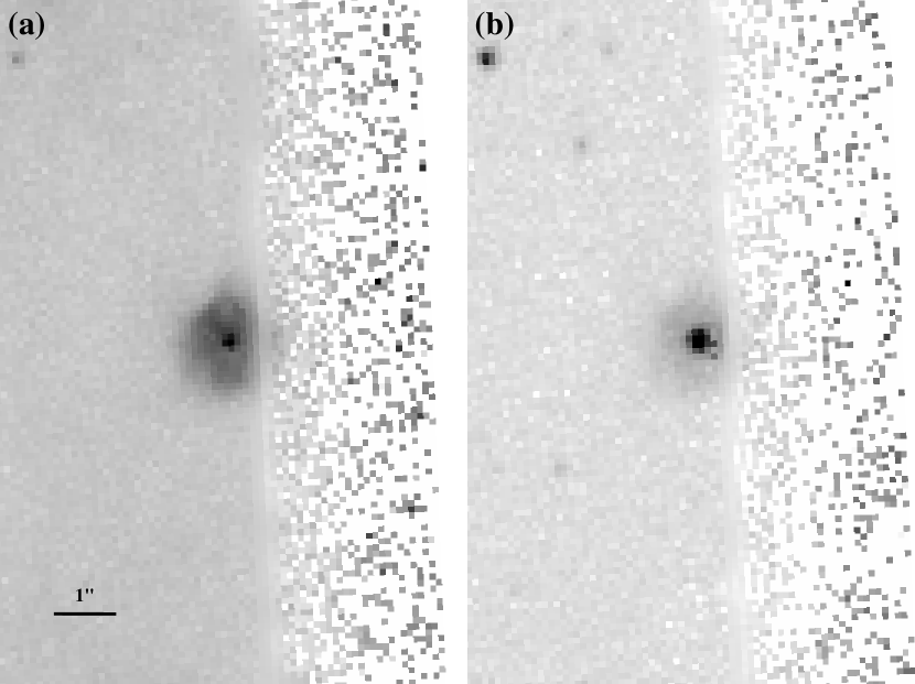
Figure 14: Close-up WFPC2 images of the small H II region associated with YSO 052207.3$-$675819.9 projected in the outskirt of N 44C. The H II region is shown in (a) H$\alpha$ (F656N) and (b) $y$ (F547M) images.

It is interesting to note that a small nebula is detected around YSO 052207.3$-$675819.9 projected in the dark cloud northwest of N 44C. A closeup of this nebula in Figure 14 shows that it is detected in the H$\alpha$ emission-line image but not in the $y$ continuum image, indicating that it is an H II region, instead of a reflection nebula. This small H II region has a size of 2$\farcs$2$\times$1$\farcs$5, or 0.53pc$\times 0.36$pc, and an average H$\alpha$ surface brightness of $1.9\times 10^{-14}$ ergs cm^-2 s^-1 arcsec^-2, corresponding to an emission measure of $9.4\times 10^{3}$ cm^-6 pc. Adopting an average diameter of 0.45 pc as the path length of H$\alpha$ emission, the rms electron density of the H II region is then $\sim 145$ cm^-3. This H II region has a size comparable to those of compact H II regions, i.e., $\lesssim 0.5$ pc, but its emission measure and rms electron density are much lower than the typical values for compact H II regions, $\gtrsim 10^{7}$ cm^-6 pc and $\gtrsim 5\times 10^{3}$ cm^-3 (Franco et al., 2000). The lower densities of this small H II region suggest that it has expanded and is more evolved than a compact H II region.

This small H II region provides an opportunity for us to use its ionization requirement to assess the spectral type of the ionizing star and compare its implied mass with that determined from the YSO SED fitting. The $UBV$ photometry of YSO 052207.3$-$675819.9, given in Table 5, suggests that its central star is a $\sim$ B2 V star reddened by $A_{V}\sim 1.3$. Applying this extinction correction to the observed H$\alpha$ flux, we obtained an H$\alpha$ luminosity of $L_{{\rm H}\alpha}$ = 3.7$\times$10³⁴ ergs s^-1, which requires an ionizing power of $Q({\rm H}^{0})=7.4\times 10^{11}~{}L_{{\rm H}\alpha}$ photons s^-1 = $2.7\times 10^{46}$ photons s^-1. This ionizing power can be provided by a main-sequence star of effective temperature of 26,200 K (Panagia, 1973), corresponding to a spectral type of B1 V (Schmidt-Kaler, 1982). The mass estimated from SED model fits for this YSO is 9–15 $M_{\odot}$, corresponding to spectral type B1-2 V. It is satisfactory that the three independent methods have produced consistent mass estimates.

This YSO in a small H II region illustrates a caveat in analyzing objects that are not fully resolved by Spitzer images. The SED model fits of YSO 052207.3$-$675819.9 infers that it is at evolutionary Stage II. The presence of a visible H II region and the visibility of the YSO in $UBV$ bands indicate that the star has little circumstellar dust and that the YSO is likely at Stage III. This discrepancy in evolutionary stage is most likely caused by the inclusion of dust emission from the H II region in the flux measurements, since it is not resolved in the ISPI and Spitzer images. It is thus important to use high-resolution images to examine the immediate surroundings of massive YSOs in order not to be mis-led by the SEDs.

7.5 The Source in N 44A: Young or Evolved?

The source 052129.7$-$675106.9 is coincident with a small compact H II region, identified as an H$\alpha$ knot and cataloged as N 44A by Henize (1956). Previously, this IR source was identified as IRAS 05216$-$6753 and classified as an H II region (Roche et al., 1987) or an obscured supergiant or AGB (Wood et al., 1992; Loup et al., 1997). Figure 15 shows that the central star of this small H II region is bright in optical wavelengths. Chen (2007) measured $V=14.17\pm 0.02$, ($B-V$) $=0.79\pm 0.03$ and ($U-B$) $=-0.64\pm 0.06$. These magnitudes and colors cannot be reproduced by any combination of normal spectral type and luminosity class. The observed ($U-B$) indicates a blue star, so the intrinsic color ($B-V$)₀ must be in the range of 0 to $-$0.3; therefore, E($B-V$) = 0.8–1.1, or $A_{v}$ = 2.5–3.4, and $M_{V}$ = $-$6.8 to $-$8, suggesting that this star is a blue supergiant of luminosity class I. It cannot be an AGB star.

We can make another independent estimate of the spectral type based on the H$\alpha$ luminosity of N 44A. Using the flux-calibrated MCELS images of N 44, we subtracted the red continuum from the H$\alpha$ image and measured a continuum-subtracted H$\alpha$ flux of 4.7$\times$10^-12 ergs s^-1 cm^-2 from N 44A. To achieve feasible ionizing power, the star has to be blue with ($B-V$)₀ $\sim$ $-$0.3, thus we adopt an extinction of $A_{v}\sim 3.4$ and find an H$\alpha$ luminosity of $1.4\times 10^{37}$ ergs s^-1. This H$\alpha$ luminosity requires the ionizing power of an O9 I star.

We thus suggest that the central star of N 44A is an O9 I star. The strong mid-IR excess of this star indicates the existence of abundant dust around the star. The anomalous combination of ($U-B$) and ($B-V$) colors may be caused by the inclusion of extra scattered light in the $U$ band. If the star is a young star, the dust and H II region would both be interstellar. If the star is an evolved star, the dust and H II region would both be ejected stellar material and show enhanced elemental abundances. The current data do not allow us to distinguish whether the central star of N 44A is a YSO or an evolved massive star, such as an LBV. High-resolution optical spectra of the H$\alpha$ and [N II] lines are needed to search for N-enriched ionized gas. If the ionized gas is enriched, the central star of N 44A is an evolved star. If the ionized gas is not enriched, the central star of N 44A must be young, otherwise its stellar wind would have blown away the small H II region.

8 Summary

We have observed the starburst region N 44 in the LMC with the Spitzer IRAC and MIPS at 3.6, 4.5, 5.8, 8.0, 24, 70, and 160 $\mu$m, CTIO Blanco 4 m telescope ISPI in $J$ and $K_{s}$ and MOSAIC in SDSS $u$ and Johnson-Cousins $BVI$ bands. Point sources were identified and their photometric measurements were made. To identify YSOs, we first constructed an [8.0] vs. [4.5]$-$[8.0] CMD and used the criteria [4.5]$-$[8.0] $\geq$ 2.0 to exclude normal and evolved stars and [8.0] $<$ 14.0$-$([4.5]$-$[8.0]) to exclude background galaxies. A total of $\sim$100 YSO candidates were identified. We then inspected the SED and close-up images of each YSO candidate in H$\alpha$, $BVIJK_{s}$, IRAC, and MIPS bands simultaneously to further identify and exclude evolved stars, galaxies, and dust clumps, resulting a final sample of 60 YSO candidates that are most likely bona fide YSOs of high or intermediate masses.

Following the classification of Classes I, II, and III for low-mass YSOs, we suggest the classification of Types I, II, and III for higher-mass YSOs, according to their SEDs. Type I YSOs are not detectable in optical to $J$ bands, and have SEDs rising beyond 24 $\mu$m. Type II YSOs become visible in optical to $J$ bands, and have SEDs peaking in the mid-MIR but falling beyond 24 $\mu$m. Type III YSOs are bright in optical, but still show excess IR emission.

To assess the physical properties of the YSOs, we use the Online SED Model Fitter (Robitaille et al., 2007) for 36 YSOs whose SEDs are reliably determined. We find the SEDs of Type I and Type I/II YSOs can be modeled well, but the SEDs of Type II and Type II/III YSOs show prominent discrepancies at 4.5 $\mu$m because the SED models of Robitaille et al. (2006) do not include the PAH emission. Some Type III YSOs show deep V- or U-shaped SEDs that require a low dust content within the central $\sim$1,000 AU, indicating a central hole in the disk. Using the SED model fits of YSOs and published spectroscopic observations of two Type III YSOs, we find at least 11 O-type YSOs in N 44.

We have examined the five UCHIIs in N 44 reported by Indebetouw et al. (2004). One is probably a mis-identified background galaxy, and the remaining four have Type I-II YSO counterparts. The stellar masses of these YSOs determined from their SED model fits agree well with the masses implied by the ionizing fluxes required by the UCHIIs. However, the SED model fits suggest envelope accretion rates much higher than the critical mass accretion rate for the formation of UCHIIs.

N 44 encompasses three molecular concentrations with different star formation histories. It is remarkable that the current formation of O-type stars is well correlated with the formation of such massive stars in the last few Myrs. The alignment of YSOs along the southwest rim of N 44’s supershell suggests that their formation may have been triggered by the expansion of the supershell. HST images show that some YSOs in N 44 are in bright-rimmed dust pillars and PDRs with PAH emission, indicating that the thermal pressure raised by photo-ionization or photo-dissociation may have triggered the star formation.

We caution that small H II regions may be associated with YSOs and thus their dust emission may contaminate the SEDs, causing uncertainties in the model fits. HST images are needed to resolve such small H II regions. Finally, we have analyzed the photometric measurements and ionizing power of the central star of N 44A, and we find the star to be O9 I star, instead of an AGB star as suggested previously.

Figure 1: MCELS H$\alpha$ and MOSAIC B-band images of N 44. (a) MCELS H$\alpha$ image of N 44, showing the nebular components A-M defined by Henize (1956) and the OB associations LH47/48/49 cataloged by Lucke & Hodge (1970). (b) MOSAIC B-band image of N 44, showing the OB associations LH47/48/49. (c) X-ray contours (Chu et al., 1993) overlaid on the MCELS H$\alpha$ image. (d) CO contours (Fukui et al., 2001) overlaid on the MCELS H$\alpha$ image.

Figure 2: IRAC and MIPS images of N 44. (a) 3.6 $\mu$m image showing stars and modest PAH emission, with OB associations LH47/48/49 labeled; (b) 8.0 $\mu$m image showing PAH and dust emissions, (c) 24 $\mu$m image showing dust emission, and (d) color composite of 3.6, 8.0, and 24 $\mu$m images. Dust shrouded objects, e.g., YSOs and AGB stars, appear red.

Figure 3: (a) [8.0] vs. [4.5]$-$[8.0] CMD of all sources detected in N 44. Known AGB stars are marked with additional open cyan squares and expected loci from AGB stellar models (Groenewegen, 2006) with filled yellow squares. The criterion to exclude normal and AGB stars is shown in short-dashed lines and that to exclude background galaxies in long-dashed lines. (b) 99 YSO candidates are found in the upper right wedge that has the minimum contamination from stars and background galaxies. These candidates have been through detail examination using multi-wavelength images and SEDs. Candidates that are most likely YSOs are marked with additional red open circles and non-YSOs with green crosses.

Figure 4: Selected SEDs of known AGB stars in N 44. (a) Carbon star LMC-BM 24-8 (Blanco & McCarthy, 1990), (b) M-type variable GRV 0523$-$6752 (Reid et al., 1988), (c) IR carbon star MSX LMC 511 (Egan et al., 2001), and (d) OH/IR star MSX LMC 516 (Egan et al., 2001).

Figure 5: (a) YSO candidates in N 44 from two studies plotted over an 8 $\mu$m image. 60 YSO candidates from this study are marked in red open circles or question mark, while 19 YSO candidates from Whitney et al. (2008) are marked in green open boxes and labeled with numbers 1–19. (b) YSO candidates in N 44 from this study and Whitney et al. (2008, abbreviated as W08 in the figure) marked on a [8.0] vs. ([4.5]-[8.0]) CMD. The latter are labeled with the same numbers as in (a). (c) SEDs of 6 YSO candidates from Whitney et al. (2008) but not included in the YSO list from this study. Two numbers are listed for each YSO candidate: the ones outside parentheses are serial numbers as labeled in (a) and (b), and the ones inside parenthesis are from Whitney et al. (2008).

Figure 6: Example YSOs (open circle) in N 44 shown in multi-wavelength images, CMD, and SED to demonstrate our classification scheme. (a) Single-source Type I YSO, (b) single-source Type II YSO, (c) single-source Type III YSO, (d) YSO in a multiple system, and (e) YSO at the peak of a dust pillar.

Fig. 6 — Continued.

Fig. 6 — Continued.

Fig. 6 — Continued.

Fig. 6 — Continued.

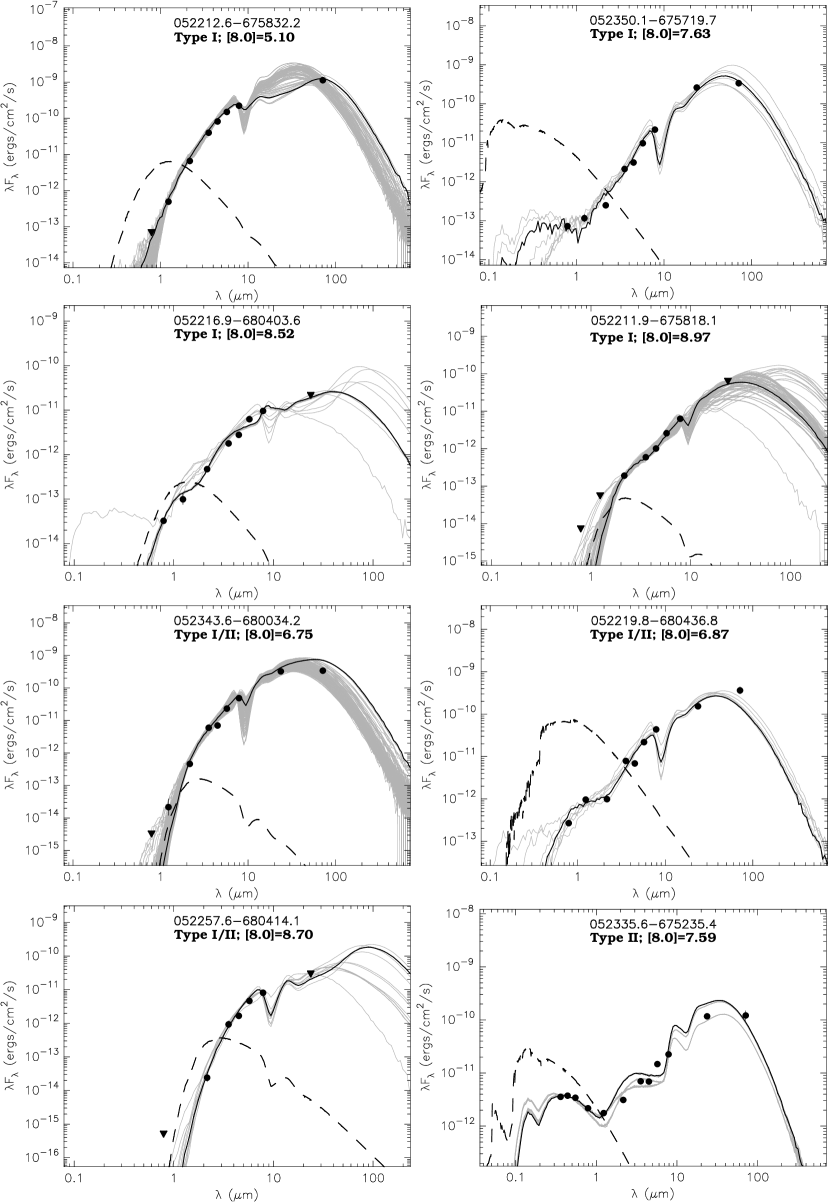
Figure 7: SEDs of 36 YSOs analyzed in this study. Filled circles are the flux values converted from magnitudes listed in Table 5. The source name, type from our empirical classification, and [8.0] mag are labeled at the top of the plot. Triangles are upper limits. Error bars are shown if larger than the data points. The solid black line shows the best-fit model, and the dashed black line illustrates the radiation from the central star reddened by the best-fit $A_{V}$. The gray lines show all acceptable models.

.

Fig. 7 — Continued.

Fig. 7 — Continued.

Fig. 7 — Continued.

Fig. 7 — Continued.

Figure 8: SEDs of 4 Type III YSOs fitted with stellar atmosphere models (Kurucz, 1993). Symbols are the same as Fig. 7.

.

Figure 9: Model SEDs of Type III YSO 052157.0$-$675700.1 with inner disk radii set as (a) 50 AU and (b) 1000 AU. Symbols are the same as Fig. 7.

.

Figure 10: Distribution of YSOs with respect to stellar and interstellar environments of N 44. The H$\alpha$ image of N 44 is shown in grey scale, overlaid with CO contours (blue lines). YSOs with different mass estimates are marked with different symbols: O-type, i.e., $M_{\star}$ Range always $\geq$ 17 $M_{\odot}$, as large red open circles; early-B type, i.e., $M_{\star}$ Range always $\geq$ 8 $M_{\odot}$, as medium red open circles; and B-type, i.e., $M_{\star}$ Range extending from intermediate to high-mass, as small red open circles. YSOs without mass estimates are shown as red pluses. The YSO candidate in N 44A has a yet-to-be-determined nature (see §7.5) and is shown as the green open triangle.

Figure 11: YSOs in the H II region N 44C. (a) and (b) show WFPC2 H$\alpha$ and IRAC 8 $\mu$m images of N 44C, overlaid with positions of YSOs (open circle) and ionizing star (open box).

Figure 12: YSOs in the H II region N 44F. (a) and (b) show WFPC2 H$\alpha$ and IRAC 8 $\mu$m images of N 44C, overlaid with positions of YSO (open circle) and ionizing star (open box).

Figure 13: YSOs in the H II region N 44H. (a) and (b) show WFPC2 H$\alpha$ and IRAC 8 $\mu$m images of N 44C, overlaid with the position of YSO (open circle).

Figure 15: YSO 052129.7$-$675106.9 (open circle) in N 44A shown in multi-wavelength images, CMD, and SED. This bright IR source, known as IRAS 05216$-$6753, was previously identified as obscured supergiant or AGB star (Wood et al., 1992; Loup et al., 1997) but the presence of compact H II region and the $UBV$ photometry suggest otherwise (see text).

Table 1: Parameters for IRAC and MIPS Photometric Measurements

	Aperture	Background	Aperture	Zero-Mag.
	Radius	Annulus	Correction	Flux
Band	(′′)	(′′)	Factor	(Jy)
IRAC 3.6 $\mu$m	3.6	3.6-8.4	1.124	277.5
4.5 $\mu$m	3.6	3.6-8.4	1.127	179.5
5.8 $\mu$m	3.6	3.6-8.4	1.143	116.6
8.0 $\mu$m	3.6	3.6-8.4	1.234	63.1
MIPS  24 $\mu$m	6	20-32	1.699	7.14
70 $\mu$m	16	39-65	2.087	0.775
160 $\mu$m	40	75-125	1.884	0.159

Table 2: Multi-wavelength Photometry of IRAC Sources in N 44

Name	R.A.	Decl.	$U$	$B$	$V$	$I$	$J$	$H$	$K_{s}$	[3.6]	[4.5]	[5.8]	[8.0]	[24]	[70]	Flag
052030.6-680316.7	80.12759	-68.05464	$\cdots$  $\cdots$	19.68 0.03	17.86 0.04	15.95 0.04	14.63 0.04	13.82 0.05	13.52 0.05	13.18 0.09	13.39 0.15	13.24 0.03	12.83 0.06	$\cdots$  $\cdots$	$\cdots$  $\cdots$	10
052030.7-674817.8	80.12783	-67.80495	$\cdots$  $\cdots$	$\cdots$  $\cdots$	$\cdots$  $\cdots$	$\cdots$  $\cdots$	$\cdots$  $\cdots$	$\cdots$  $\cdots$	$\cdots$  $\cdots$	$\cdots$  $\cdots$	$\cdots$  $\cdots$	$\cdots$  $\cdots$	14.46 0.21	$\cdots$  $\cdots$	$\cdots$  $\cdots$	10
052030.7-680353.3	80.12783	-68.06480	$\cdots$  $\cdots$	21.44 0.12	20.61 0.12	19.30 0.07	$\cdots$  $\cdots$	$\cdots$  $\cdots$	$\cdots$  $\cdots$	17.08 0.07	$\cdots$  $\cdots$	16.41 0.47	$\cdots$  $\cdots$	$\cdots$  $\cdots$	$\cdots$  $\cdots$	10
052030.7-674946.3	80.12787	-67.82953	$\cdots$  $\cdots$	20.57 0.05	19.69 0.04	$\cdots$  $\cdots$	$\cdots$  $\cdots$	$\cdots$  $\cdots$	$\cdots$  $\cdots$	16.83 0.06	16.78 0.09	$\cdots$  $\cdots$	$\cdots$  $\cdots$	$\cdots$  $\cdots$	$\cdots$  $\cdots$	0
052030.7-674436.7	80.12789	-67.74352	21.49 0.45	20.57 0.06	19.46 0.05	18.44 0.06	$\cdots$  $\cdots$	$\cdots$  $\cdots$	$\cdots$  $\cdots$	$\cdots$  $\cdots$	17.20 0.10	$\cdots$  $\cdots$	$\cdots$  $\cdots$	$\cdots$  $\cdots$	$\cdots$  $\cdots$	10
052030.7-675920.8	80.12793	-67.98911	19.46 0.05	18.31 0.01	17.05 0.02	$\cdots$  $\cdots$	14.89 0.04	14.20 0.07	14.10 0.07	13.90 0.17	13.94 0.01	13.81 0.04	13.50 0.08	$\cdots$  $\cdots$	$\cdots$  $\cdots$	0

Note. — Table 2 is presented in its entirety in the electronic edition of the Astrophysical Journal. A portion of is shown here for guidance regarding its form and content. Column 1: source name. Columns 2-3: right ascension and declination in degrees. Columns 4-16: photometric measurements of 13 bands from $U$ to 70 $\mu$m in magnitudes. Column 17: data used for $UBVI$ photometry: 0 - $UBV$ from Chen (2007), 10 - $UBVI$ from MCPS.

Table 3: Archival HST WFPC2 Observations of Fields in N 44

R.A.	Decl.			Exp. Time
(J2000)	(J2000)	Program ID/PI	Filter	(s)
05 21 45.3	-68 06 13.5	7553/MacKenty	F300W	$1\times 2900$
05 21 49.8	-67 54 59.1	6698/Chu	F656N	$2\times 500$
			F673N	$2\times 500$
05 21 58.4	-68 06 36.2	7553/MacKenty	F300W	$1\times 2900$
05 22 07.9	-67 59 13.0	6623/Garnett	F502N	$3\times 700$
			F547M	$2\times 80$
			F656N	$3\times 700$
			F675W	$2\times 80$
05 22 35.7	-67 58 12.8	6698/Chu	F656N	$2\times 500$
			F673N	$2\times 500$
05 22 54.9	-68 01 41.9	6540/Schulte-Ladbeck	F656N	$2\times 5$, $2\times 30$, $2\times 500$
05 23 40.2	-67 59 46.8	6253/MacKenty	F300W	$1\times 160$, $1\times 260$

Table 4: Effective Wavelength and Zero-Magnitude Flux of $UBVIJHK_{s}$ Bands

	$U$	$B$	$V$	$I$	$J$	$H$	$K_{s}$
Effective
Wavelength ($\mu$m)	0.367	0.436	0.545	0.797	1.235	1.662	2.159
0th mag
$F_{\nu}$ (Jy)	1780	4000	3600	2420	1594	1024	666.8

Note. — Adopted from Bessell & Murdin (2000) for $UBVI$, Cohen et al. (2003) for $JHK_{s}$.

Table 5: Multi-wavelength Photometry of YSO Candidates Selected from CMD Criteria

Name	No	$U$	$B$	$V$	$I$	$J$	$H$	$K_{s}$
(1)	(2)	(3)	(4)	(5)	(6)	(7)	(8)	(9)
		[3.6]	[4.5]	[5.8]	[8.0]	[24]	[70]	Flag	Class.	Remarks
		(10)	(11)	(12)	(13)	(14)	(15)	(16)	(17)	(18)
052042.0-674307.7	96	… …	… …	… …	… …	16.06 0.11	15.04 0.11	14.71 0.12
		13.85 0.01	13.81 0.01	13.61 0.04	11.64 0.02	9.30 0.25	… …	0	G
052046.6-675255.1	15	… …	… …	… …	19.23 0.01	17.78 0.12	… …	15.95 0.06
		12.45 0.01	12.46 0.08	9.53 0.02	7.81 0.01	3.88 0.01	-0.79 0.10	11	T2
052106.8-675715.9	99	19.76 0.17	20.29 0.06	18.85 0.16	… …	16.61 0.18	15.44 0.16	15.18 0.20
		14.23 0.02	13.99 0.01	… …	11.79 0.03	… …	… …	0	G
052117.5-680204.6	41	… …	… …	… …	19.66 0.02	17.85 0.15	… …	15.98 0.07
		13.36 0.01	13.25 0.01	10.52 0.04	8.73 0.02	5.40 0.01	-0.26 99.9	11	G? YSC?
052120.7-674706.6	31	… …	… …	… …	… …	… …	… …	… …
		13.03 0.02	12.96 0.03	10.21 0.02	8.51 0.02	5.34 0.01	… …	0	D
052120.7-674725.5	74	17.39 0.07	18.50 0.06	17.81 0.08	17.25 0.08	… …	… …	… …
		13.65 0.09	13.18 0.07	11.30 0.12	9.54 0.13	… …	… …	0	S	on IR D
052120.9-674716.7	82	… …	… …	… …	… …	… …	… …	… …
		13.96 0.07	13.20 0.04	… …	10.40 0.21	… …	… …	0	D
052120.9-680217.6	98	… …	22.50 0.50	21.91 0.18	19.94 0.11	… …	… …	… …
		14.95 0.04	13.94 0.02	12.70 0.23	11.68 0.22	7.80 99.9	… …	0	ES?
052122.0-674729.0	5	… …	… …	… …	18.77 0.01	17.12 0.12	… …	14.88 0.04
		12.08 0.06	11.76 0.06	9.27 0.03	7.44 0.01	1.86 0.01	-2.17 0.06	11	YSO+RN?
052126.2-674742.1	71	17.62 0.03	18.03 0.02	17.91 0.02	19.43 0.01	17.76 0.15	… …	16.39 0.07
		13.54 0.03	13.38 0.02	… …	9.47 0.05	5.92 99.9	… …	11	T2, mul	in MC
052127.2-675915.1	92	15.37 0.01	15.43 0.01	14.86 0.01	… …	13.71 0.02	13.38 0.04	13.35 0.04
		13.08 0.09	13.38 0.01	12.50 0.07	11.24 0.09	… …	… …	0	blue S
052129.7-675106.9	1	14.32 0.01	14.96 0.01	14.17 0.01	14.07 0.01	13.00 0.03	12.02 0.03	10.46 0.02
		8.03 0.01	6.96 0.01	5.83 0.01	4.12 0.01	sat. …	-2.95 0.04	10	ES
052133.3-674420.8	97	16.36 0.07	17.11 0.02	16.85 0.12	17.93 0.01	16.52 0.06	… …	15.21 0.05
		… …	13.82 0.01	… …	11.65 0.05	7.98 0.01	… …	11	mul YSOs?
052135.5-675500.2	86	… …	18.49 0.02	17.29 0.01	… …	15.09 0.06	14.34 0.06	14.20 0.08
		14.04 0.26	13.94 0.10	12.75 0.15	10.89 0.13	… …	… …	0	S	in DR
052136.0-675443.4	65	17.16 0.05	17.75 0.02	17.28 0.04	17.31 0.01	16.93 0.06	… …	16.10 0.03
		13.65 0.27	13.01 0.20	11.48 0.19	9.32 0.07	… …	… …	11	T2/3	tip of DC
052136.3-674643.2	89	… …	… …	… …	21.49 0.12	20.48 0.67	… …	17.54 0.08
		15.30 0.14	13.65 0.05	12.49 0.09	11.06 0.16	5.36 0.01	… …	11	mul YSOs
052136.6-675449.4	75	… …	… …	… …	… …	… …	… …	… …
		13.85 0.10	13.87 0.17	11.44 0.15	9.54 0.06	4.04 0.01	… …	0	D
052138.0-674630.3	72	… …	… …	… …	19.30 0.24	17.95 0.11	… …	16.75 0.03
		13.72 0.24	13.91 0.07	11.20 0.09	9.52 0.04	4.80 0.01	… …	11	T2
052141.9-675324.1	63	20.40 0.25	20.42 0.10	19.68 0.13	19.62 0.02	18.13 0.17	… …	16.47 0.05
		13.90 0.05	13.81 0.04	11.00 0.07	9.26 0.04	5.32 0.02	… …	11	T2, mul?
052144.5-674541.5	45	… …	21.01 0.10	19.88 0.13	20.58 0.03	19.15 0.20	… …	15.41 0.04
		13.38 0.01	13.36 0.01	10.65 0.01	8.91 0.01	5.87 0.03	0.37 99.9	11	YSC?
052147.1-675656.7	17	14.05 0.01	14.91 0.01	15.30 0.01	14.86 0.02	14.94 0.03	… …	14.31 0.03
		12.07 0.04	11.89 0.06	9.63 0.02	7.84 0.01	2.54 0.01	… …	11	T3
052152.8-675449.5	91	13.98 0.01	14.94 0.01	14.97 0.01	… …	14.69 0.06	14.43 0.07	14.25 0.10
		13.68 0.18	13.39 0.19	12.62 0.08	11.18 0.11	… …	… …	0	S
052154.2-674737.1	90	… …	… …	… …	21.54 0.04	19.73 0.33	… …	16.58 0.06
		14.41 0.03	13.50 0.23	12.54 0.21	11.10 0.10	… …	… …	11	T2, mul?	in DC
052155.3-674730.2	61	… …	… …	… …	20.36 0.02	18.48 0.18	… …	16.14 0.01
		12.90 0.09	11.77 0.04	10.49 0.04	9.20 0.02	5.00 0.01	… …	11	T2, mul
052155.3-675634.9	46	18.54 0.07	19.47 0.03	19.01 0.04	18.49 0.01	17.47 0.12	… …	15.36 0.01
		12.90 0.10	12.77 0.13	10.61 0.06	8.89 0.04	4.90 99.9	… …	11	T2/3
052157.0-675700.1	77	13.43 0.01	14.36 0.01	14.42 0.01	14.32 0.01	14.66 0.03	… …	14.64 0.01
		14.29 0.12	13.50 0.27	11.90 0.15	9.96 0.10	3.52 99.9	… …	11	T3: O8.5V+N
052157.5-675618.5	59	… …	… …	… …	… …	… …	… …	… …
		13.60 0.10	13.40 0.09	10.95 0.10	9.16 0.07	4.27 0.05	… …	0	D
052157.9-675625.5	68	11.96 0.01	12.95 0.01	13.12 0.01	… …	13.32 0.03	13.28 0.04	13.16 0.04
		12.57 0.10	12.45 0.12	10.83 0.09	9.37 0.08	… …	… …	0	S: O7III((f))
052158.2-675554.2	44	17.62 0.03	18.42 0.02	18.32 0.02	17.82 0.02	17.18 0.11	… …	15.12 0.01
		12.34 0.07	11.79 0.07	10.27 0.05	8.81 0.04	5.12 99.9	… …	11	T2/3
052159.0-674437.2	76	19.57 0.15	19.55 0.07	18.81 0.10	18.55 0.01	17.57 0.14	… …	16.36 0.08
		14.13 0.02	13.79 0.01	11.43 0.01	9.71 0.01	6.68 0.04	… …	11	T2, mul?
052159.6-675721.7	79	12.82 0.01	13.78 0.01	14.03 0.01	14.78 0.02	14.35 0.03	… …	14.23 0.03
		13.43 0.10	12.86 0.10	… …	10.09 0.24	… …	… …	11	T3: O7.5V+N
052159.6-675715.6	78	… …	… …	… …	… …	… …	… …	… …
		14.32 0.36	13.90 0.30	11.89 0.27	10.05 0.26	… …	… …	0	D
052200.4-675745.0	25	… …	… …	… …	… …	… …	… …	… …
		13.01 0.13	13.49 0.33	10.23 0.11	8.37 0.11	… …	… …	0	D
052201.9-675732.5	56	… …	17.37 0.11	17.00 0.23	19.48 0.12	18.05 0.23	… …	16.17 0.10
		13.59 0.33	13.39 0.36	10.57 0.21	9.07 0.25	… …	… …	11	YSO, mul?	in DC
052202.0-675758.2	13	… …	… …	… …	22.52 0.39	21.06 99.9	… …	17.66 0.15
		12.69 0.12	11.50 0.08	9.36 0.05	7.77 0.03	… …	… …	11	T2	in DC
052202.2-675753.6	11	… …	… …	… …	18.89 0.02	17.16 0.11	… …	14.93 0.04
		12.36 0.11	11.95 0.12	9.40 0.04	7.67 0.03	1.75 0.02	… …	11	T2
052202.3-674657.5	33	… …	… …	… …	20.81 0.10	18.28 0.19	… …	15.96 0.04
		13.18 0.17	12.86 0.03	10.35 0.06	8.51 0.03	2.41 0.01	… …	11	YSO	in DC
052202.8-674701.9	14	19.31 0.14	20.14 0.13	18.74 0.14	18.53 0.01	17.11 99.9	… …	15.18 0.01
		12.12 0.06	11.75 0.07	9.54 0.03	7.77 0.02	2.01 99.9	-2.39 99.9	11	T2	at tip of DC
052203.1-674703.5	16	17.26 0.10	17.95 0.05	17.66 0.11	17.28 0.01	16.42 0.07	… …	15.41 0.03
		12.10 0.02	11.78 0.02	9.64 0.03	7.81 0.03	… …	… …	11	T2
052203.4-675746.9	24	… …	… …	… …	… …	… …	… …	16.58 0.09
		12.76 0.14	11.78 0.08	10.01 0.07	8.28 0.04	1.74 99.9	… …	11	T1/2?	in DC
052203.9-675743.7	52	… …	… …	… …	18.78 0.02	18.25 0.19	… …	16.19 0.07
		12.95 0.20	11.82 0.10	10.77 0.17	8.98 0.10	… …	… …	11	T2	in DC
052204.1-674709.7	73	17.74 0.06	18.39 0.05	18.48 0.06	18.14 0.12	… …	… …	… …
		13.92 0.04	13.94 0.04	11.24 0.04	9.52 0.05	… …	… …	0	S	on IR D
052204.8-675744.6	42	… …	… …	… …	19.40 0.03	17.88 0.14	… …	15.62 0.05
		13.29 0.27	13.00 0.31	10.87 0.33	8.76 0.20	… …	… …	11	T2/3	at edge of DC
052204.9-675720.6	62	… …	… …	… …	… …	… …	… …	… …
		13.45 0.12	13.42 0.12	11.16 0.23	9.22 0.20	… …	… …	0	D
052204.9-675801.6	36	20.70 0.23	19.87 0.05	19.00 0.03	… …	… …	… …	… …
		13.08 0.16	12.61 0.11	10.25 0.14	8.54 0.06	2.08 0.02	… …	0	D
052205.2-675741.6	38	… …	… …	… …	22.18 0.37	20.08 0.64	… …	16.25 0.08
		13.39 0.25	12.79 0.15	… …	8.61 0.23	… …	… …	11	mul YSOs	in DC
052205.3-675748.5	21	… …	… …	… …	… …	… …	… …	17.22 0.13
		13.12 0.26	12.97 0.35	9.88 0.06	8.13 0.04	2.06 99.9	… …	11	T2?	in DC
052206.4-675659.2	28	… …	… …	… …	19.34 0.36	17.74 0.15	… …	15.16 0.04
		12.28 0.07	11.64 0.06	9.98 0.04	8.41 0.02	4.37 99.9	… …	11	T2
052207.3-675819.9	19	17.73 0.01	18.35 0.01	18.16 0.01	17.51 0.01	16.71 0.09	… …	15.38 0.05
		12.30 0.07	11.87 0.07	9.71 0.03	8.01 0.02	2.79 99.9	… …	11	T3	in HII
052207.3-675826.8	26	… …	… …	… …	21.20 99.9	19.66 99.9	… …	15.21 0.04
		11.99 0.07	10.54 0.02	9.43 0.03	8.38 0.04	3.05 99.9	… …	11	T2	in DC
052207.7-675649.4	85	18.68 0.08	18.91 0.04	19.03 0.04	… …	… …	… …	… …
		14.19 0.07	13.94 0.10	12.50 0.07	10.69 0.07	… …	… …	0	S	in DR
052208.5-675821.3	30	… …	… …	… …	… …	… …	… …	… …
		12.93 0.04	12.46 0.04	10.16 0.06	8.45 0.03	2.90 0.04	… …	0	D
052208.6-675805.5	51	… …	… …	… …	19.35 0.05	17.83 0.15	… …	15.24 0.04
		12.32 0.08	11.68 0.08	10.42 0.10	9.01 0.09	4.44 0.25	… …	11	mul YSOs
052208.6-675921.9	70	18.00 0.02	18.75 0.01	18.68 0.02	18.57 0.01	17.61 0.14	… …	16.43 0.09
		13.79 0.04	13.83 0.03	11.10 0.08	9.38 0.05	5.92 0.14	… …	11	T2, mul?
052208.8-675325.2	60	18.61 0.06	18.98 0.03	18.68 0.04	18.05 0.01	17.37 0.11	… …	16.23 0.04
		13.35 0.11	13.13 0.15	10.79 0.04	9.19 0.02	5.63 0.02	… …	11	T2 + T3/S
052208.9-674703.4	93	17.39 0.08	16.74 0.02	15.82 0.04	14.81 0.04	14.11 0.03	13.61 0.04	13.52 0.04
		13.33 0.01	13.38 0.18	12.64 0.09	11.37 0.14	… …	… …	0	blue S
052211.9-675818.1	48	… …	… …	… …	22.79 0.27	19.55 0.31	… …	16.72 0.09
		14.01 0.13	12.69 0.17	10.92 0.10	8.97 0.05	2.04 99.9	… …	11	T1	in DC
052212.0-674713.9	80	21.47 0.53	21.01 0.11	20.55 0.13	20.05 0.02	18.00 0.15	… …	15.89 0.03
		13.63 0.17	12.74 0.10	11.40 0.09	10.10 0.05	6.43 0.01	… …	11	T2
052212.3-675813.4	49	… …	… …	… …	18.63 0.01	17.35 0.11	… …	15.37 0.04
		12.99 0.17	12.24 0.12	10.61 0.10	8.97 0.07	… …	… …	11	T2/3	in DC
052212.6-675832.2	2	… …	… …	… …	20.34 99.9	17.24 0.12	… …	12.87 0.01
		9.44 0.01	7.92 0.01	6.51 0.01	5.10 0.01	sat. …	-3.85 0.08	11	T1
052216.7-675837.7	55	… …	… …	… …	… …	… …	… …	… …
		13.92 0.14	13.57 0.15	10.85 0.10	9.07 0.09	… …	… …	0	D
052216.8-680428.3	66	… …	… …	… …	… …	… …	… …	… …
		13.91 0.06	13.92 0.08	11.12 0.04	9.32 0.05	4.96 0.04	… …	0	D peak
052216.9-680403.6	34	… …	… …	… …	21.22 0.08	18.98 0.27	… …	15.73 0.06
		12.81 0.09	11.59 0.04	9.96 0.03	8.52 0.03	4.01 0.01	… …	11	T1
052217.8-680432.9	69	… …	… …	… …	… …	… …	… …	… …
		13.80 0.06	13.68 0.08	11.07 0.06	9.36 0.06	… …	… …	0	D
052218.9-675813.8	64	… …	… …	… …	… …	… …	… …	… …
		… …	13.84 0.12	11.21 0.15	9.31 0.13	… …	… …	0	D
052219.8-680436.8	4	… …	18.24 0.08	18.16 0.13	18.93 0.14	16.51 0.09	… …	14.93 0.04
		11.20 0.04	10.61 0.03	8.60 0.02	6.87 0.01	1.93 0.01	-2.62 0.07	11	T1/2	in DC
052221.0-680515.3	94	… …	… …	… …	… …	… …	… …	… …
		15.35 0.02	13.85 0.28	12.81 0.26	11.38 0.11	8.32 0.21	… …	0	ES?
052227.7-675412.8	37	… …	… …	… …	21.85 0.22	18.85 0.24	… …	15.92 0.04
		13.05 0.13	12.95 0.15	10.32 0.06	8.55 0.03	4.20 0.04	… …	11	T2?	in DC
052229.1-675339.5	50	16.11 0.03	17.04 0.04	16.65 0.02	16.21 0.01	15.95 0.06	… …	15.12 0.02
		13.08 0.10	13.05 0.15	10.68 0.05	9.00 0.02	5.34 0.03	… …	11	T3, mul
052230.4-675443.9	18	16.11 0.01	16.75 0.01	16.40 0.01	… …	14.84 0.08	14.42 0.10	13.62 0.11
		11.93 0.06	11.38 0.06	… …	7.88 0.09	2.38 0.01	-2.69 0.09	0	S	in HII
052231.8-680319.2	27	18.75 0.10	19.65 0.06	19.59 0.06	19.44 0.03	17.73 0.14	… …	15.70 0.06
		12.75 0.10	12.33 0.09	10.11 0.05	8.40 0.03	3.85 0.01	… …	11	T2	in DC?
052232.7-680301.7	53	… …	… …	… …	19.45 0.01	17.26 0.11	… …	15.06 0.04
		13.06 0.10	12.69 0.09	10.90 0.07	9.02 0.03	4.42 0.01	… …	11	T2, mul	in DC
052241.4-675508.2	84	16.15 0.01	16.19 0.01	15.55 0.01	… …	14.12 0.03	13.62 0.04	13.57 0.05
		13.37 0.12	13.33 0.17	12.02 0.16	10.52 0.06	… …	… …	0	S
052242.0-675500.5	81	… …	… …	… …	20.86 0.03	18.51 0.22	… …	16.12 0.01
		14.04 0.04	13.21 0.02	11.66 0.13	10.24 0.10	5.50 0.02	… …	11	T2
052249.0-680111.1	67	… …	… …	… …	… …	… …	… …	… …
		13.93 0.16	13.76 0.11	11.20 0.16	9.36 0.09	… …	… …	0	D
052249.2-680129.0	23	17.66 0.02	18.41 0.02	17.98 0.02	15.84 0.03	15.88 0.02	… …	14.77 0.03
		12.51 0.07	12.34 0.09	9.97 0.01	8.26 0.02	4.27 0.01	… …	11	T2, mul
052251.0-680401.0	35	… …	… …	… …	… …	… …	… …	… …
		13.16 0.08	13.21 0.06	10.32 0.07	8.52 0.04	… …	… …	0	D
052251.7-680436.7	39	18.35 0.06	19.07 0.02	18.76 0.03	… …	… …	… …	… …
		12.98 0.11	12.80 0.11	10.41 0.09	8.63 0.06	… …	… …	0	S	near DC
052253.7-680434.8	20	… …	… …	… …	… …	… …	… …	… …
		12.85 0.14	12.57 0.16	9.82 0.06	8.12 0.04	2.01 0.02	… …	0	D
052254.6-680424.3	10	… …	… …	… …	… …	… …	… …	… …
		12.04 0.06	11.90 0.08	9.52 0.10	7.65 0.03	… …	… …	0	D
052254.9-680422.2	6	… …	… …	… …	… …	… …	… …	… …
		11.93 0.05	11.67 0.07	9.32 0.04	7.49 0.07	1.64 0.01	… …	0	D
052255.2-680409.5	8	17.16 0.06	18.31 0.04	18.00 0.04	17.18 0.01	15.63 0.05	… …	14.28 0.03
		12.08 0.07	11.70 0.07	9.37 0.03	7.63 0.02	2.35 0.01	… …	11	T2
052255.4-680431.6	22	… …	20.69 0.03	20.15 0.03	… …	… …	… …	… …
		13.15 0.12	13.05 0.14	… …	8.25 0.12	… …	… …	0	D
052256.8-680406.9	12	19.23 0.07	20.00 0.04	19.52 0.05	18.61 0.01	16.75 0.09	… …	14.99 0.04
		12.25 0.09	12.26 0.12	9.46 0.04	7.76 0.02	3.29 0.01	… …	11	T2
052257.6-680414.1	40	… …	… …	… …	… …	… …	… …	18.97 0.28
		13.52 0.24	12.14 0.09	10.28 0.06	8.70 0.04	3.65 99.9	… …	11	T1/2
052259.0-680346.3	83	… …	… …	… …	18.97 0.24	17.84 0.14	… …	15.61 0.05
		13.16 99.9	12.49 99.9	11.61 0.16	10.46 0.14	5.49 0.05	… …	11	T2
052308.7-680006.8	43	… …	… …	… …	20.50 0.03	18.69 0.18	… …	16.28 0.04
		13.53 0.17	12.94 0.15	10.61 0.07	8.78 0.04	3.51 0.01	… …	11	YSC	in DC
052309.4-680205.5	58	18.48 0.01	18.91 0.01	18.63 0.01	… …	… …	… …	… …
		13.69 0.04	13.78 0.04	10.88 0.05	9.15 0.05	6.04 0.02	… …	0	D peak
052311.4-680040.9	54	… …	… …	… …	… …	… …	… …	… …
		13.52 0.06	13.41 0.04	10.81 0.06	9.07 0.05	4.62 0.03	… …	0	D peak
052315.1-680017.0	57	13.40 0.01	14.19 0.01	14.10 0.01	13.86 0.01	13.81 0.04	… …	13.69 0.05
		13.02 0.17	12.62 0.17	11.20 0.12	9.10 0.06	2.32 0.01	… …	11	T3	in HII
052318.0-675938.6	32	… …	… …	… …	… …	16.34 0.14	15.94 0.20	14.70 99.9
		13.15 0.10	12.73 0.07	10.25 0.06	8.51 0.04	… …	… …	0	D
052318.0-675942.8	47	… …	… …	… …	… …	… …	… …	… …
		13.49 0.16	12.94 0.24	10.59 0.09	8.94 0.06	… …	… …	0	D peak
052331.5-680107.9	29	17.64 0.03	18.27 0.02	17.59 0.02	16.85 0.01	16.12 0.06	… …	15.41 0.05
		12.91 0.12	12.83 0.16	10.19 0.06	8.42 0.04	4.44 0.01	… …	11	T2
052335.6-675235.4	7	16.58 0.02	17.19 0.03	16.95 0.02	16.66 0.01	15.86 0.06	… …	13.69 0.02
		11.33 0.02	10.60 0.02	9.03 0.01	7.59 0.01	2.22 0.01	-1.43 0.08	11	T2
052340.6-680528.5	87	14.94 0.03	15.73 0.07	15.73 0.02	15.52 0.01	15.56 0.07	… …	15.20 0.18
		14.16 0.04	13.45 0.04	12.67 0.05	10.95 0.04	4.90 0.01	0.58 0.23	11	T3 or B[e] S
052343.6-680034.2	3	… …	… …	… …	23.65 99.9	20.63 0.62	… …	15.76 0.05
		11.50 0.04	10.59 0.03	8.54 0.01	6.75 0.01	1.12 0.01	-2.55 0.07	11	T1/2
052343.9-680056.1	88	… …	… …	… …	21.66 0.08	18.69 0.24	… …	16.97 0.11
		14.16 0.05	13.71 0.03	12.40 0.09	11.00 0.17	… …	… …	11	mul YSOs
052350.1-675719.7	9	… …	… …	… …	20.35 0.04	18.81 0.21	… …	16.43 0.07
		12.62 0.09	11.46 0.04	9.48 0.03	7.63 0.01	1.35 0.01	-2.54 0.06	11	T1
052351.1-675326.6	95	… …	… …	… …	… …	… …	… …	… …
		14.54 0.01	13.60 0.22	12.52 0.02	11.54 0.12	9.07 0.07	… …	0	ES?

Note. — Column 1: source name. Column 2: Ranking of the brightness at 8 $\mu$m. Columns 3-16: photometric measurements of 13 bands from $U$ to 70 $\mu$m in magnitudes. Measurements with uncertainties of $99.9$ are the upper brightness limits as they include fluxes from neighbors or backgrounds. Column 17: data used for $IJHK$ photometry: 0 – $I$ from MCPS and $JHK$ from 2MASS catalog, 10 – $I$ from 4m Mosaic data and $JHK$ from 2MASS catalog, 11 – $I$ from 4m Mosaic data and $JHK$ from 4m ISPI data. Column 18 and 19: classification and remarks: D – diffuse emission, DC – dark cloud, DR – dusty region, ES – evolved star, G – background galaxy, MC – molecular cloud, mul – multiple, N – nebula, RN – reflection nebula, S – star, T1/2/3 – Type I/II/III YSO, YSC – young star cluster.

Table 6: YSO Candidates in N 44 in Two Catalogs

	W08	Source Name	Offset		Classification
No.	No.	in This Study	$\Delta\alpha$	$\Delta\delta$	W08	This Study
1	530	052042.1-675255.0	$-$0.41	0.21	YSO	G cut
2	546	052116.2-674511.7	$-$0.09	$-$0.28	YSO	E cut
3	552	052129.7-675106.9	$-$0.07	0.27	PN	III? E?
4	557	052147.1-675656.7	$-$0.34	0.07	YSO_hp	III
5	563	052155.3-674730.2	$-$0.52	$-$0.13	YSO_hp	II
6	565	052159.0-674437.2	$-$0.12	0.12	YSO	II
7	566	052202.0-675758.2	$-$0.25	0.19	YSO	II
8	572	052207.3-675826.8	0.05	$-$0.03	YSO	II
9	574	052211.5-675401.9	$-$0.23	0.35	YSO	G cut
10	576	052212.0-674713.9	$-$0.44	0.01	YSO_hp	II
11	579	052212.6-675832.2	$-$0.10	$-$0.06	YSO	I
12	581	052216.9-680403.6	$-$0.28	$-$0.22	YSO_hp	I
13	598	052249.2-680129.0	$-$0.61	0.10	YSO	II
14	604	052259.0-680346.3	$-$0.37	0.23	YSO	II
15	606	052302.2-680400.1	$-$0.47	0.34	YSO	G cut
16	609	052308.7-680006.8	$-$0.67	0.23	YSO	YSC
17	613	052318.5-680045.5	$-$0.52	$-$0.19	YSO	E cut
18	616	052335.6-675235.4	$-$0.19	$-$0.27	YSO_hp	II
19	622	052351.3-680712.3	$-$0.81	0.10	YSO_hp	E cut

Table 7: Inferred Physical Parameters from SED Fits to YSOs

			M∗		Physical Parameters of the Best-Fit Model
	[8.0]		Range	Stage	M∗	T∗	R∗	Age	$\dot{M}_{\rm env}$	$\dot{M}_{\rm disk}$	$M_{\rm disk}$	$i$	$L_{\rm tot}$	AV
Source Name	(mag)	Type	($M_{\odot}$)	Range	($M_{\odot}$)	(K)	($R_{\odot}$)	(yr)	($M_{\odot}$/yr)	($M_{\odot}$/yr)	($M_{\odot}$)	($\arcdeg$)	($L_{\odot}$)	(mag)	Remark
052212.6-675832.2	5.10	I	20-50	I	26	16000	37.7	8E+03	7.6E$-$03	0.0E+00	0.0E+00	18	92000	6.1	DC, UCHII
052350.1-675719.7	7.63	I	17-25	I	21	33000	7.5	3E+04	1.2E$-$03	0.0E+00	0.0E+00	56	62000	1.1	DC
052216.9-680403.6	8.52	I	8-15	I,II	8	16000	8.8	2E+05	1.0E$-$05	1.8E$-$07	6.0E$-$02	41	4300	7.2
052211.9-675818.1	8.97	I	8-28	I,II	28	4200	300.0	1E+03	5.9E$-$04	0.0E+00	0.0E+00	56	26000	2.1	DC
052343.6-680034.2	6.75	I/II	17-37	I,II	20	18000	23.3	2E+04	5.9E$-$03	0.0E+00	0.0E+00	18	53000	27.5	DC, UCHII
052219.8-680436.8	6.87	I/II	17-24	I	21	8000	93.7	5E+03	3.9E$-$04	0.0E+00	0.0E+00	49	33000	1.9	DC, UCHII
052257.6-680414.1	8.70	I/II	10-16	I,II	16	8400	56.6	1E+04	6.5E$-$03	0.0E+00	0.0E+00	18	15000	29.7	CO peak
052335.6-675235.4	7.59	II	14-17	II,III	17	33000	5.3	9E+05	1.7E$-$08	6.7E$-$11	1.9E$-$06	18	30000	0.9
052255.2-680409.5	7.63	II	13-18	I,II	13	30000	4.6	3E+05	4.0E$-$06	7.8E$-$07	3.6E$-$01	81	15000	0.0	UCHII
052202.2-675753.6	7.67	II	17-36	I,II	18	6400	125.0	6E+03	1.4E$-$04	8.8E$-$06	9.4E$-$02	87	23000	0.2	DC?
052256.8-680406.9	7.76	II	11-12	I	12	29000	4.3	2E+05	1.7E$-$05	1.8E$-$08	2.3E$-$02	87	11000	0.7
052202.0-675758.2	7.77	II	9	II	9	24000	3.7	2E+06	0.0E+00	6.1E$-$07	6.8E$-$02	56	4100	9.9	DC
052202.8-674701.9	7.77	II	8-15	I,II,III	15	8900	47.3	1E+04	2.0E$-$04	3.0E$-$06	6.9E$-$02	49	13000	0.1	DC tip
052046.6-675255.1	7.81	II	17	II	17	33000	5.3	1E+06	0.0E+00	8.7E$-$07	1.5E$-$01	87	32000	0.0
052203.1-674703.5	7.81	II	8-14	I,III	8	16000	8.8	2E+05	1.0E$-$05	1.8E$-$07	6.0E$-$02	41	4300	0.4
052207.3-675826.8	8.38	II	7-25	I,II	11	4400	76.8	5E+03	1.8E$-$04	1.8E$-$04	4.0E$-$01	18	2700	7.8	DC
052231.8-680319.2	8.40	II	8-15	I,II	8	12000	13.9	1E+05	8.9E$-$05	5.2E$-$10	8.0E$-$04	18	3200	2.9	DC?
052206.4-675659.2	8.41	II	8-15	I,II	13	5900	78.2	1E+04	4.2E$-$03	4.0E$-$06	2.2E$-$01	18	6600	1.2
052331.5-680107.9	8.42	II	8	I	8	16000	8.8	2E+05	1.0E$-$05	1.8E$-$07	6.0E$-$02	69	4300	0.9
052203.9-675743.7	8.98	II	8-15	I,II	8	22000	3.4	8E+05	5.0E$-$07	5.5E$-$06	1.2E$-$01	31	2700	2.0	DC
052138.0-674630.3	9.52	II	9-10	I	9	7000	31.4	4E+04	4.5E$-$04	1.2E$-$05	2.4E$-$02	18	2200	3.5
052212.0-674713.9	10.10	II	2-9	I	9	5100	48.7	3E+04	1.3E$-$03	5.1E$-$07	8.7E$-$02	18	1400	1.9
052242.0-675500.5	10.24	II	5-10	I	9	6200	31.4	5E+04	6.3E$-$05	4.8E$-$07	6.1E$-$02	41	1300	3.6
052259.0-680346.3	10.46	II	4-11	I,II	6	18000	3.6	5E+05	1.0E$-$05	2.9E$-$08	1.7E$-$03	18	1200	1.9
052204.8-675744.6	8.76	II/III	8-33	I,II,III	9	6000	43.2	3E+04	6.1E$-$05	3.9E$-$09	2.4E$-$03	31	2200	0.7	DC edge
052158.2-675554.2	8.81	II/III	5-14	I,III	12	7100	51.8	2E+04	3.8E$-$03	1.7E$-$07	2.5E$-$03	18	6100	1.0
052155.3-675634.9	8.89	II/III	8-9	I,II	8	22000	3.4	4E+05	6.2E$-$05	8.2E$-$08	1.6E$-$02	63	2300	0.5
052212.3-675813.4	8.97	II/III	5-28	I,II,III	12	7100	51.8	2E+04	3.8E$-$03	1.7E$-$07	2.5E$-$03	18	6100	1.0	superposed on DC
052136.0-675443.4	9.32	II/III	6-11	II,III	6	13000	5.8	5E+05	2.3E$-$07	1.9E$-$09	3.2E$-$03	41	890	0.1	dust pillar tip
052129.7-675106.9	4.12	III	34	II	34	42000	7.8	5E+05	1.2E$-$06	1.1E$-$10	4.6E$-$04	41	160000	0.0	$\sim$O9I, this study
052147.1-675656.7	7.84	III	17	III	17	33000	5.3	1E+06	0.0E+00	8.7E$-$13	1.0E$-$06	81	32000	0.1
052207.3-675819.9	8.01	III	9-15	II	9	25000	3.7	3E+05	3.0E$-$06	1.8E$-$08	1.1E$-$03	41	4600	0.4
052315.1-680017.0	9.10	III	20-21	III	21	36000	5.9	1E+06	0.0E+00	4.7E$-$12	2.4E$-$06	75	50000	0.0	B0-O5V
052157.0-675700.1	9.96	III	9	I	9	9200	20.1	6E+04	9.6E$-$05	9.9E$-$06	5.5E$-$01	18	2800	0.0	O8.5V
052159.6-675721.7	10.09	III	16	III	16	32000	5.1	1E+06	0.0E+00	1.5E$-$11	4.7E$-$07	31	25000	0.0	O7.5V
052340.6-680528.5	10.95	III	12	III	12	28000	4.4	2E+06	0.0E+00	9.3E$-$14	7.4E$-$07	87	11000	0.0	B[e]

Table 8: Properties of YSOs with UCHIIs

			Stage	$M_{\star}$	Spec.	Spec.	$\dot{M}_{\rm env}$	$\dot{M}_{\rm crit}$
UCHII	YSO ID	Type	Range	($M_{\odot}$)	Type	Type	($M_{\odot}$/yr)	($M_{\odot}$/yr)
B0522$-$5800	052212.6$-$675832.2	I	I	26	O7-8 V	O7 V	7.6E$-$03	4.1E$-$05
B0523$-$6806(NE)	052343.6$-$680034.2	I/II	I,II	20	O8-9 V	O9 V	5.9E$-$03	1.8E$-$05
B0523$-$6806(SW)	052219.8$-$680436.8	I/II	I	21	O8-9 V	O8.5 V	3.9E$-$04	2.2E$-$05
B0523$-$6806	052255.2$-$680409.5	II	I,II	13	B1-2 V	B0 V	4.0E$-$06	1.0E$-$05

References

- Allamandola et al. (1989) Allamandola, L. J., Tielens, G. G. M., & Barker, J. R. 1989, ApJS, 71, 733
- Beech & Mitalas (1994) Beech, M., & Mitalas, R. 1994, ApJS, 95, 517
- Bernasconi & Maeder (1996) Bernasconi, P. A., & Maeder, A. 1996, A&A, 307, 829
- Bessell & Murdin (2000) Bessell, M., & Murdin, P. 2000, Encyclopedia of Astronomy and Astrophysics
- Blanco & McCarthy (1990) Blanco, V. M., & McCarthy, M. F. 1990, AJ, 100, 674
- Brott & Hauschildt (2005) Brott, I., & Hauschildt, P. H. 2005, in ESA Special Publication, Vol. 576, The Three-Dimensional Universe with Gaia, ed. C. Turon, K. S. O’Flaherty, & M. A. C. Perryman, 565
- Buchanan et al. (2006) Buchanan, C. L., et al. 2006, AJ, 132, 1890
- Calvet et al. (2005) Calvet, N., et al. 2005, ApJ, 630, L185
- Caulet et al. (2008) Caulet, A., Gruendl, R. A., & Chu, Y.-H. 2008, ApJ, 678, 200
- Cesaroni et al. (2007) Cesaroni, R., Galli, D., Lodato, G., Walmsley, C. M., & Zhang, Q. 2007, in Protostars and Planets V, ed. B. Reipurth, D. Jewitt, & K. Keil, 197
- Chen (2007) Chen, C.-H. R. 2007, PhD thesis
- Chin et al. (1997) Chin, Y.-N., Henkel, C., Whiteoak, J. B., Millar, T. J., Hunt, M. R., & Lemme, C. 1997, A&A, 317, 548
- Chu et al. (1993) Chu, Y.-H., Mac Low, M.-M., Garcia-Segura, G., Wakker, B., & Kennicutt, Jr., R. C. 1993, ApJ, 414, 213
- Chu et al. (2005) Chu, Y.-H., et al. 2005, ApJ, 634, L189
- Churchwell (2002) Churchwell, E. 2002, ARA&A, 40, 27
- Cohen et al. (2003) Cohen, M., Wheaton, W. A., & Megeath, S. T. 2003, AJ, 126, 1090
- Draine & Li (2007) Draine, B. T., & Li, A. 2007, ApJ, 657, 810
- Egan et al. (2001) Egan, M. P., Van Dyk, S. D., & Price, S. D. 2001, AJ, 122, 1844
- Elmegreen (1998) Elmegreen, B. G. 1998, in ASP Conf. Ser. 148: Origins, ed. C. E. Woodward, J. M. Shull, & H. A. Thronson, Jr., 150
- Fazio et al. (2004) Fazio, G. G., et al. 2004, ApJS, 154, 10
- Feast (1999) Feast, M. 1999, in IAU Symp. 190: New Views of the Magellanic Clouds, ed. Y.-H. Chu, N. Suntzeff, J. Hesser, & D. Bohlender, 542
- Franceschini et al. (2005) Franceschini, A., et al. 2005, AJ, 129, 2074
- Franco et al. (2000) Franco, J., Kurtz, S. E., García-Segura, G., & Hofner, P. 2000, Ap&SS, 272, 169
- Fukui et al. (2001) Fukui, Y., Mizuno, N., Yamaguchi, R., Mizuno, A., & Onishi, T. 2001, PASJ, 53, L41
- Gordon et al. (2005) Gordon, K. D., et al. 2005, PASP, 117, 503
- Gouliermis et al. (2006) Gouliermis, D., Brandner, W., & Henning, T. 2006, ApJ, 636, L133
- Groenewegen (2006) Groenewegen, M. A. T. 2006, A&A, 448, 181
- Gruendl & Chu (2008) Gruendl, R. A., & Chu, Y.-H. 2008, ApJS, submitted
- Harvey et al. (2006) Harvey, P. M., et al. 2006, ApJ, 644, 307
- Hatziminaoglou et al. (2005) Hatziminaoglou, E., et al. 2005, AJ, 129, 1198
- Henize (1956) Henize, K. G. 1956, ApJS, 2, 315
- Hester et al. (1996) Hester, J. J., et al. 1996, AJ, 111, 2349
- Hillenbrand et al. (1992) Hillenbrand, L. A., Strom, S. E., Vrba, F. J., & Keene, J. 1992, ApJ, 397, 613
- Hollenbach & Tielens (1997) Hollenbach, D. J., & Tielens, A. G. G. M. 1997, ARA&A, 35, 179
- Humphreys & Davidson (1994) Humphreys, R. M., & Davidson, K. 1994, PASP, 106, 1025
- Indebetouw et al. (2004) Indebetouw, R., Johnson, K. E., & Conti, P. 2004, AJ, 128, 2206
- Jones et al. (2005) Jones, T. J., Woodward, C. E., Boyer, M. L., Gehrz, R. D., & Polomski, E. 2005, ApJ, 620, 731
- Kurucz (1993) Kurucz, R. 1993, ATLAS9 Stellar Atmosphere Programs and 2 km/s grid. Kurucz CD-ROM No. 13. Cambridge, Mass.: Smithsonian Astrophysical Observatory, 1993., 13
- Lada (1987) Lada, C. J. 1987, in IAU Symp. 115: Star Forming Regions, ed. M. Peimbert & J. Jugaku, 1
- Li & Draine (2001) Li, A., & Draine, B. T. 2001, ApJ, 554, 778
- Li & Draine (2002) —. 2002, ApJ, 576, 762
- Lonsdale et al. (2003) Lonsdale, C. J., et al. 2003, PASP, 115, 897
- Loup et al. (1997) Loup, C., Zijlstra, A. A., Waters, L. B. F. M., & Groenewegen, M. A. T. 1997, A&AS, 125, 419
- Lucke & Hodge (1970) Lucke, P. B., & Hodge, P. W. 1970, AJ, 75, 171
- Magnier et al. (1996) Magnier, E. A., Chu, Y.-H., Points, S. D., Hwang, U., & Smith, R. C. 1996, ApJ, 464, 829
- Meixner et al. (2006) Meixner, M., et al. 2006, AJ, 132, 2268
- Mizuno et al. (2001) Mizuno, N., et al. 2001, PASJ, 53, 971
- Nazé et al. (2002) Nazé, Y., Chu, Y.-H., Guerrero, M. A., Oey, M. S., Gruendl, R. A., & Smith, R. C. 2002, AJ, 124, 3325
- Nota et al. (2006) Nota, A., et al. 2006, ApJ, 640, L29
- Oey & Massey (1995) Oey, M. S., & Massey, P. 1995, ApJ, 452, 210
- Panagia (1973) Panagia, N. 1973, AJ, 78, 929
- Pottasch (1993) Pottasch, S. R. 1993, in Infrared Astronomy, ed. A. Mampaso, M. Prieto, & F. Sanchez, 63
- Reid et al. (1988) Reid, N., Glass, I. S., & Catchpole, R. M. 1988, MNRAS, 232, 53
- Ressler & Barsony (2003) Ressler, M. E., & Barsony, M. 2003, ApJ, 584, 832
- Rice et al. (2003) Rice, W. K. M., Wood, K., Armitage, P. J., Whitney, B. A., & Bjorkman, J. E. 2003, MNRAS, 342, 79
- Rieke et al. (2004) Rieke, G. H., et al. 2004, ApJS, 154, 25
- Robitaille et al. (2007) Robitaille, T. P., Whitney, B. A., Indebetouw, R., & Wood, K. 2007, ApJS, 169, 328
- Robitaille et al. (2006) Robitaille, T. P., Whitney, B. A., Indebetouw, R., Wood, K., & Denzmore, P. 2006, ApJS, 167, 256
- Roche et al. (1987) Roche, P. F., Aitken, D. K., & Smith, C. H. 1987, MNRAS, 228, 269
- Rowan-Robinson et al. (1986) Rowan-Robinson, M., Lock, T. D., Walker, D. W., & Harris, S. 1986, MNRAS, 222, 273
- Rowan-Robinson et al. (2005) Rowan-Robinson, M., et al. 2005, AJ, 129, 1183
- Schmidt-Kaler (1982) Schmidt-Kaler, T. 1982, in Landolt-Börnstein New Series, Group 6, Volume 2b, Stars and Star Clusters, ed. K. Schaifers & H. H. Voigt (Berlin: Springer)
- Siess et al. (2000) Siess, L., Dufour, E., & Forestini, M. 2000, A&A, 358, 593
- Simon et al. (2007) Simon, J. D., et al. 2007, ApJ, 669, 327
- Skrutskie et al. (2006) Skrutskie, M. F., et al. 2006, AJ, 131, 1163
- Smith & The MCELS Team (1999) Smith, R. C., & The MCELS Team. 1999, in IAU Symp. 190: New Views of the Magellanic Clouds, ed. Y.-H. Chu, N. Suntzeff, J. Hesser, & D. Bohlender, 28
- Stahl et al. (1984) Stahl, O., Wolf, B., Leitherer, C., Zickgraf, F.-J., Krautter, J., & de Groot, M. 1984, A&A, 140, 459
- Stahler et al. (2000) Stahler, S. W., Palla, F., & Ho, P. T. P. 2000, Protostars and Planets IV, 327
- Thompson et al. (2002) Thompson, R. I., Smith, B. A., & Hester, J. J. 2002, ApJ, 570, 749
- van Boekel et al. (2004) van Boekel, R., Waters, L. B. F. M., Dominik, C., Dullemond, C. P., Tielens, A. G. G. M., & de Koter, A. 2004, A&A, 418, 177
- Whitney et al. (2004a) Whitney, B. A., Indebetouw, R., Bjorkman, J. E., & Wood, K. 2004a, ApJ, 617, 1177
- Whitney et al. (2003) Whitney, B. A., Wood, K., Bjorkman, J. E., & Cohen, M. 2003, ApJ, 598, 1079
- Whitney et al. (2004b) Whitney, B. A., et al. 2004b, ApJS, 154, 315
- Whitney et al. (2008) —. 2008, AJ, 136, 18
- Will et al. (1997) Will, J.-M., Bomans, D. J., & Dieball, A. 1997, A&AS, 123, 455
- Wood et al. (1992) Wood, P. R., Whiteoak, J. B., Hughes, S. M. G., Bessell, M. S., Gardner, F. F., & Hyland, A. R. 1992, ApJ, 397, 552
- Yorke & Sonnhalter (2002) Yorke, H. W., & Sonnhalter, C. 2002, ApJ, 569, 846
- Zaritsky et al. (2004) Zaritsky, D., Harris, J., Thompson, I. B., & Grebel, E. K. 2004, AJ, 128, 1606
- Zinnecker & Yorke (2007) Zinnecker, H., & Yorke, H. W. 2007, ARA&A, 45, 481