Dark energy constraints from cosmic shear power spectra: impact of intrinsic alignments on photometric redshift requirements
Abstract
Cosmic shear constrains cosmology by exploiting the apparent alignments of pairs of galaxies due to gravitational lensing by intervening mass clumps. However galaxies may become (intrinsically) aligned with each other, and with nearby mass clumps, during their formation. This effect needs to be disentangled from the cosmic shear signal to place constraints on cosmology. We use the linear intrinsic alignment model as a base and compare it to an alternative model and data. If intrinsic alignments are ignored then the dark energy equation of state is biased by per cent. We examine how the number of tomographic redshift bins affects uncertainties on cosmological parameters and find that when intrinsic alignments are included two or more times as many bins are required to obtain 80 per cent of the available information. We investigate how the degradation in the dark energy figure of merit depends on the photometric redshift scatter. Previous studies have shown that lensing does not place stringent requirements on the photometric redshift uncertainty, so long as the uncertainty is well known. However, if intrinsic alignments are included the requirements become a factor of three tighter. These results are quite insensitive to the fraction of catastrophic outliers, assuming that this fraction is well known. We show the effect of uncertainties in photometric redshift bias and scatter. Finally we quantify how priors on the intrinsic alignment model would improve dark energy constraints.
Subject headings:
large-scale structure of Universe – cosmological parameters – surveys1. Introduction
**footnotetext: E-mail: sarah.bridle@ucl.ac.ukThe tidal gravitational field of density inhomogeneities in the universe distorts the images of distant galaxies. This so-called ‘cosmic shear’ results in correlations in the observed ellipticities of the distant galaxies, a signal which depends upon the geometry of the universe and the matter power spectrum (Blandford et al., 1991; Miralda-Escude, 1991; Kaiser, 1992). The first detections of cosmic shear made in 2000 (Bacon et al., 2000; Kaiser et al., 2000; Van Waerbeke et al., 2000; Wittman et al., 2000) demonstrated its value as a cosmological tool. Future generations of multi-color imaging surveys will cover thousands of square degrees and have the potential to measure the dark matter power spectrum with unprecedented precision in three dimensions at low redshift which is not possible with the CMB. This is important because dark energy only starts to dominate at low redshift. Ultimately, cosmic shear data can improve constraints on the dark energy equation of state from the CMB by over an order of magnitude Hu (2002).
The great promise and exactitude of cosmic shear has necessitated the design of instruments expressly geared towards measurement of the tiny lensing-induced distortions. It has also motivated improvements in techniques to account for changes in galaxy shapes due to the atmosphere and telescope optics. Furthermore it has prompted careful consideration of any potential cosmological contaminants of the cosmic shear signal. Intrinsic alignments of galaxies are a potential contaminant and fall into two categories. The first is intrinsic-intrinsic galaxy alignments (II correlations), which may arise during the galaxy formation process since neighboring galaxies reside in a similar tidal field (e.g. Crittenden et al. (2001)). The second, related, effect is a cross-term between intrinsic ellipticity and cosmic shear (GI correlations, Hirata and Seljak (2004)), whereby the intrinsic shape of a galaxy is correlated with the surrounding density field, which in turn contributes to the lensing distortion of more distant galaxies. The net effect of this is an induced anti-correlation between galaxy ellipticities, leading to a suppression of the total measured signal.
Intrinsic galaxy alignment has been subject to numerous analytic, numerical and observational studies [e.g. Croft and Metzler (2000); Heavens et al. (2000a); Crittenden et al. (2001); Mackey et al. (2002); Jing (2002); Heymans et al. (2004a); Hirata et al. (2004); Bridle and Abdalla (2007)]. Brown et al. (2003) and Heymans et al. (2004a) detected an II signal in the SuperCOSMOS data. Mandelbaum et al. (2006) used in excess of a quarter of a million spectroscopic galaxies from SDSS to obtain constraints on intrinsic alignments, with no detection of an II signal. Since II correlations only operate when galaxies are physically close, this contaminant is relatively straightforward to deal with by down-weighting or removing those pairs if redshifts are well known (King and Schneider, 2002; Heymans and Heavens, 2003; Takada and White, 2004) or by fitting parameterized models relying on the different behavior of lensing and II in redshift space (King and Schneider, 2003).
The first observational detection of a large-scale density-galaxy ellipticity correlation was made by Mandelbaum et al. (2006), using the same SDSS sample noted above; their detection is robust and is present on scales up to 60 Mpc. They estimate that the amplitude of the GI correlation could cause existing deep surveys to underestimate the linear amplitude of fluctuations by as much as . The GI signal is dominated by the brightest galaxies, possibly due to these being BCGs (brightest cluster galaxies) aligned with the cluster ellipticity. Hirata et al. (2007) perform a more detailed characterization of this effect, including a higher redshift sample of LRGs (luminous red galaxies). They estimate that results on from future cosmic shear surveys may be biased by around 10 per cent. Using N-body simulations, Heymans et al. (2006a) estimate that in a survey with median depth , the GI signal can contribute up to 10% of the lensing signal on scales up to 20 arcmin.
As noted by Hirata and Seljak (2004), unlike II correlations, GI correlations are not localized in redshift, and hence their removal is more complex. Given that the GI term has been observationally detected we cannot ignore it. Hirata and Seljak (2004) suggested that the dependence of the GI signal on redshift could be used to distinguish it from cosmic shear. King (2005) showed that projecting the signal into a set of template functions would enable the lensing, II and GI signals to be isolated, again harnessing their different dependence on redshift.
In this paper we aim to remove the intrinsic alignment contamination of cosmic shear by simultaneously measuring cosmological and intrinsic alignment parameters from shear power spectra. The increased number of fitted parameters may degrade constraints on cosmological parameters. Here we focus on the requirements this places on photometric redshift quality.
The planned future imaging surveys will observe at least hundreds of millions of galaxies. It will not be possible to obtain spectroscopic redshifts for them all. Therefore it is planned to rely on ‘photometric redshifts’: estimates calculated from galaxy luminosities in several observing bands. The resulting redshift accuracy is critically dependent on the number of observing bands used. Equally important for measurement of cosmological parameters is the existence of a representative sample with spectroscopic redshifts which allows the redshift accuracy to be quantified. It is important to plan now for these future observations since decisions are being made about which observing bands to use. Furthermore it may be necessary to mount a dedicated observing campaign if more spectroscopic redshifts are needed than are currently planned.
In practice additional information may be included in the fit to help offset the degradation due to using many free parameters to encapsulate the intrinsic alignment model. This may come from measurements such as those by Mandelbaum et al. (2006) and Hirata et al. (2007). Any additional information on at least the functional form of the intrinsic alignment contributions from theory would also be a great help. This information could be included by applying priors to the intrinsic alignment power spectra in the simultaneous analysis. We investigate the size of prior required to improve constraints relative to the self-calibration regime.
In section 2 we introduce our fiducial intrinsic alignment model. Section 3 shows how dark energy constraints are affected by varying parameters within this model. In section 4 we show the requirements this places on photometric redshift quality. Finally in section 5 we consider the effect of priors on photometric redshift and intrinsic alignment parameters.
2. Intrinsic Alignment Model
In this paper we attempt to simultaneously measure the intrinsic alignment and cosmological model from cosmic shear power spectra. We therefore have to parameterize the sources of the intrinsic alignments in some sufficiently flexible yet physically reasonable way. We also need to define a fiducial model for intrinsic alignments to put into our simulation of the future observations.
We assume a catalogue of source galaxy positions and shears which is divided up into a number of bins in redshift, with a number per unit comoving distance for bin . For convenience this is normalized as . The lensing efficiency function for lensing a mass at redshift for source redshift bin may then be written as
| (1) |
where and are the comoving distances from the observer to the deflector and source respectively. We assume a flat universe throughout. is the matter density parameter, is the Hubble constant and is the speed of light.
As detailed in Hirata and Seljak (2004) the shear power spectra between redshift bins and come from the sum of three terms
| (2) |
where the first term is the usual gravitational lensing contribution, the second term arises from the intrinsic alignments of physically close galaxies and the final term arises from the intrinsic alignment of a galaxy with a mass which lenses a more distant galaxy.
In this paper we consider only E mode power spectra, since the lensing and intrinsic alignment contributions to the B mode power spectra are both very small (for the model considered).
These contributions can be written in terms of underlying power spectra as
| (3) | |||||
| (4) | |||||
| (5) |
where . The first power spectrum is simply the (non-linear) matter power spectrum at the deflector redshift. For simplicity in this paper we use the Peacock and Dodds (1996) method to modify a Ma (1996) power spectrum (containing baryon supression but no wiggles).
The remaining two power spectra are not well known. We use perturbations around the linear alignment model normalized approximately to data. We detail our assumptions and compare them to data below.
2.1. Fiducial intrinsic-intrinsic term (II)
The intrinsic-intrinsic term describes the extent to which nearby galaxies are aligned with each other, for example due to common tidal forces during their formation. For this paper we simplify the linear alignment model presented in Catelan et al. (2001) and developed in Hirata et al. (2004) to use only the first term of Hirata et al. (2004) Equation 16, written
| (6) |
where is a normalization constant, and is the linear theory matter power spectrum. where is the growth factor normalized to unity at the present day. is the mean matter density of the Universe as a function of redshift. We estimate the value of by matching to the power spectra in Figure 2 of Hirata et al. (2004) and estimate . Hirata et al. (2004) chose their by comparison with SuperCOSMOS Brown et al. (2003).
The term we ignore is roughly an order of magnitude smaller than the term we include. This can be seen in Hirata et al. (2004) by examining the B-mode II power spectrum which is of the same order as the term we ignore. Indeed from the figures it can be seen that the B-mode II power spectrum is typically an order of magnitude below the E-mode II power spectrum.
The linear alignment model might be a reasonable approximation on large scales, but clearly makes a number of simplifying assumptions on small scales. Inspired by the remark in Hirata et al. (2007) (Section 8) we attempt to make a more realistic model by inserting the full non-linear matter power spectrum into 6
| (7) |
We refer to this throughout as the non-linear linear alignment model. As noted in Hirata et al. (2007) this “model” has no grounding in theory. It might not even be closer to the truth: galaxies may become more or less aligned due to non-linear interactions. However we find this “model” matches slightly better to other models and data and therefore we use it as our default throughout.
The HRH* model for the intrinsic alignment correlation function was proposed by Heavens et al. (2000b) and improved by Heymans et al. (2004b). This model predicts the average intrinsic alignment on the sky between two galaxies, as a function of the three dimensional separation between the galaxies. Heymans et al. (2004b) and Mandelbaum et al. (2006) placed constraints on the amplitude of this model using COMBO-17 and SDSS data respectively.
These correlation functions may be projected along the line of sight to produce quantities, and , which are closely related to the II power spectrum in Eq. 5 by
| (8) |
where is the separation between pairs of galaxies in the plane of the sky, and throughout are Bessel functions of the first kind. Here is the correlation of galaxy shapes using the component of shear aligned along the line joining the two galaxies. There is another correlation function which comes from the shear components at 45 degrees to the line joining the two galaxies. In the above we have followed HRH* and assumed that these two correlation functions are the same () and thus simplified Hirata et al. (2004) Equation 10 to write Eq. 8.
The HRH* model prediction for is given by
| (9) |
where is the factor to convert measured ellipticity to shear, is the separation between galaxy pairs along the line of sight, and . The galaxy clustering correlation function is described by and , and and are free parameters of the HRH* model.
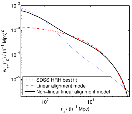
Mandelbaum et al. (2006) follow Heymans et al. (2004b) by fitting to data and using , Mpc, and Mpc. For their method . We calculate using these parameters and the best fit to SDSS L3-L6 of . We follow Section 4.3 of Mandelbaum et al. (2006) by using a range of integration of Mpc. The result is shown by the dotted line in Fig. 1. Our x axis range covers the range of data used for the fit.
We use the linear alignment model to predict by inverting Eq. 8:
| (10) |
We calculate this at a redshift of to match the mean redshift of the SDSS sample. This is shown in Fig. 1 by the dot-dashed line, which uses the linear theory matter power spectrum (Eq. 6 in Eq. 10). The solid line shows the result when the non-linear theory matter power spectrum is used (Eq. 7 in Eq. 10).
It can be seen that the linear alignment model predictions have a similar amplitude to the HRH* fit. This is not surprising since the amplitude of the linear alignment model was taken from Hirata et al. (2004) who made a fit to the Heymans et al. (2004b) data which is not far from the Mandelbaum et al. (2006) result. The linear alignment model is lower than the HRH* model on small scales and larger on scales Mpc. However the HRH* model was developed for small scale correlations therefore the discrepancy with the linear alignment model on large scales is not a concern (it was based on an approximation to the density correlation function that only applies on small scales). Both the linear alignment model and the HRH* model fit comfortably within the error bars of Mandelbaum et al. (2006). We note that the non-linear linear alignment model is closer to the HRH* model.
2.2. Fiducial shear-intrinsic term(GI)
As shown in Hirata et al. (2004), the linear alignment model predicts for the GI underlying power spectrum
| (11) |
where is the same number as in Eq. 6. We also define
| (12) |
where is the full non-linear matter power spectrum which may help to encapsulate non-linear effects on smaller scales. For example it was shown in Bridle and Abdalla (2007) that even if there were no tidal interactions between galaxies, there will still be a shear-intrinsic correlation on small scales if galaxies are aligned with their own dark matter halos.
We compare this to the SDSS results by Hirata et al. (2007), who measure the real space galaxy-shape correlation function projected along the line of sight which is defined by
| (13) |
where is the radial shear of one galaxy relative to another, averaged over all pairs of galaxies of a separation on the sky and along the line of sight (see Hirata et al. (2007) equation 10 for the estimator they use).
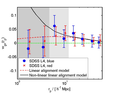
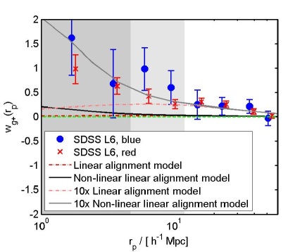
The Hirata et al. (2007) results for luminosity bins L4 and L6 are shown in Fig. 2. We show their results for L4 because it has the largest number of galaxies and therefore will be most typical of future cosmic shear surveys. We show results for L6 (which contains the most luminous galaxies) because there is a detection of the signal in this band and we would like to compare the shape of the linear alignment model prediction with the observations.
We can more easily predict theoretically the mass-shape correlation function which can be related to the corresponding power spectrum by
| (14) |
(Hirata et al., 2007, Equation 23). Hirata et al. (2007) convert from to by multiplying by the galaxy-mass bias of the sample which we take from their Table 5. We use the effective redshift values from this table and the same cosmological model as Hirata et al. (2007) to calculate and convert it to shown in Fig. 2.
The L4 data points fit very nicely over the fiducial linear alignment model predictions. Note that the dark (light) grey shaded regions block over the data points that Hirata et al. (2007) did not use for their most (least) conservative cuts when fitting models. It is not trivial that these data agree with the model. The amplitude in the linear alignment model was chosen to match observations of the II power spectrum. The agreement with the GI data is some support for the linear alignment model which links the two.
The L6 data points are much above our fiducial linear alignment model predictions. This is because we are aiming to use parameters correct for the majority of the population, whereas L6 is a very bright sample. We multiply the predictions by a factor of 10 to compare their shapes with the data. We see that there is a slightly better fit when using the non-linear matter power spectrum in the linear alignment model equation (Eq. 12). It was effectively this comparison which originally led Hirata et al. (2007) to suggest using the non-linear power spectrum.
On scales less than Mpc the L4 results appear to agree slightly better with the linear theory predictions than those from the non-linear matter power spectrum. However the error bars are large and these data points are not used in the model fitting by Hirata et al because the bias is non-linear on these scales. We expect the non-linear alignment model to be more difficult to disentangle from the cosmic shear signal because it has a similar shape, as a function of scale. We show in Fig. 7 the results for both models and find them to be quite similar in their photometric redshift requirements.
2.3. Implications for our fiducial survey
For the remainder of this paper we use as our fiducial cosmological model the best fit to WMAP3 (Spergel, 2006). This has a normalized Hubble constant , total matter density , baryon density , fluctuation amplitude normalization and primordial fluctuation spectral index . We use fiducial dark energy parameters and where the dark energy equation of state as a function of scale factor is given by (Chevallier and Polarski, 2001; Linder, 2003). We use a maximum angular power spectrum multipole throughout.
Throughout we use a fiducial survey similar to DUNE†††The Dark UNiverse Explorer (DUNE) http://www.dune-mission.net/ and LSST‡‡‡The Large Synoptic Sky Survey (LSST) http://www.lsst.org, the ‘shallow’ survey described in Amara and Refregier (2006). This covers 20,000 square degrees to a depth of with galaxies per square arcminute which can be used for shear measurements. As in Amara and Refregier (2006) we use the redshift distribution given by Smail et al. (1994) using and . By default we divide this survey up into twenty redshift bins, binned to have an equal number of source galaxies in each bin. As discussed below we use to parameterize the photometric redshift error, and by default use .
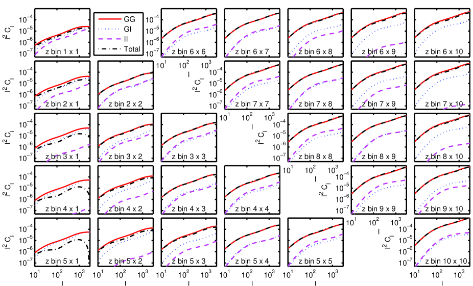
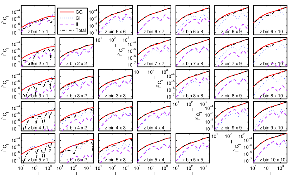
To show the size of the intrinsic alignment contributions we plot in Fig. 3 some of the power spectra for a survey divided into 10 source redshift bins. The GI and II contributions to the lensing power spectra are typically about an order of magnitude lower than the GG contribution. For illustration we show only the results for a high redshift subset of the bins. However, for the auto correlation of the lowest redshift bin the II signal is the largest contribution to the total power spectrum. When cross correlating the lowest redshift bin with the 2nd and 3rd lowest bins, the GI term can become larger than the GG term and the total power spectrum negative.
Despite the small size of the intrinsic alignment contribution, we must note that the effect on the power spectra of the cosmological parameters, including the dark energy equation of state, can be very small and therefore these contributions are very important. Huterer et al. (2006) give an approximate expression (equation 24 of their paper) for the dependence of the lensing power spectra on cosmological parameters which includes . Therefore an increase in the fluctuation normalization parameter by 1 per cent increases the power spectra by around 3 per cent. A change in of 1 per cent (e.g. to ) typically changes the lensing power spectrum by about per cent (decrease). With future surveys we are aiming to measure the dark energy equation of state to of order 1 per cent.
We simulate power spectra that include intrinsic alignment contributions but find the best fit cosmological parameters that would be obtained if intrinsic alignments were mistakenly ignored (GG). The purpose is to assess the importance of bothering to consider intrinsic alignments for future studies. We make the simplistic assumption that changes in the cosmic shear power spectra are linear in the cosmological parameters. If this assumption were correct then Fisher matrix uncertainties would also be correct, so it is a useful investigation to compare with predicted cosmological parameter uncertainties.
Given the numbers above, it is not surprising that if we fit to the lensing power spectra mistakenly ignoring the GI and II contributions we mis-estimate the fluctuation amplitude parameter by , in agreement with previous studies (see the upper section of Table 1 for details). From the numbers above we expect the effect on the dark energy equation of state to be about a factor of 10 larger. Indeed we find that the dark energy equation of state is mis-estimated by around 50 per cent for a non-tomographic (2D) analysis.
| (marginalised) | ||||
|---|---|---|---|---|
| GG+II | 1.7% | 0.28 | ||
| 2D | GG+GI | 0.78 | 6.8 | |
| GG+II+GI | 0.55 | 0.15 | ||
| GG+II | 3.2% | 2.1 | 5.8 | |
| 3D | GG+GI | 0.03 | 1.5 | |
| GG+II+GI | 0.3% | 2.5 | 4.3 |
This mis-estimate only applies if all cosmological parameters are known except the dark energy equation of state. In fact we find that if several cosmological parameters are fitted simultaneously the mis-estimate becomes even worse, as near-degeneracy directions are exploited in an attempt to match the shape of the GG+GI+II power spectra using the GG spectra alone. Therefore if our fiducial model is roughly correct it would be a disaster to ignore intrinsic alignments in studies aiming to measure the dark energy equation of state.
Table LABEL:tab:biases shows that the final overestimate of the dark energy equation of state is 15% for a 2D non-tomographic analysis, and over 400% for a 10 bin tomography analysis. Note that these numbers are only indicative, since they assume that the likelihood surface is Gaussian with a constant curvature, which will not be a good approximation so far from the fiducial model.
The simplest way we can hope to remove the II contribution is to use only cross-power spectra and to ignore the auto-correlations. Fig. 3 reminds us that more than just the auto-correlations may need to be removed if the photometric redshifts are not perfect and many redshift bins are used. For 10 photometric redshift bins and the II contribution is non-negligible even when cross correlating non-neighboring bins (e.g. ). Further, due to the photometric redshift errors the GI contribution is non-negligible even for auto-correlations.
2.4. Parameterizing intrinsic alignment uncertainties
On obtaining shear power spectra from new data we will attempt to estimate cosmological parameters. However, since the linear alignment model is approximate we cannot rely on it being correct. It seems unlikely that the galaxy formation process will one day be understood so well that we can use it to perfectly remove intrinsic alignments. We can hope to measure the contaminant from analyses such as those of Mandelbaum et al. (2006) and Hirata et al. (2007). However it will still be necessary to use a parameterized model to fit to the data points, and there will remain some uncertainty on the model parameters due to the error bars on the data points.
For this paper we parameterize perturbations around the linear alignment model and show the effect of fitting these free parameters simultaneously with the cosmological parameters. This follows the approach indicated in section 7 of the technical appendix of Albrecht et al. (2006). Our most basic perturbation is to assume some unknown amplitude and redshift dependence, which is different for each of II and GI:
| (15) |
where is or .
However this assumes that the scale dependence of the models is well known, whereas we have seen that there is still great uncertainty (e.g. compare the HRH model with the linear alignment model in Fig. 1). Further, the scale will likely deviate in a different way from the linear alignment model at different redshifts. In principle we have two unknown 2d functions and multiplying each of the power spectra for the II and GI terms:
| (16) |
To parameterize the using a finite number of parameters we use bins in and bins in redshift and linearly interpolate in the logs of , and . That is,
| (17) |
where
| (18) | |||||
| (19) |
and runs from to and runs from to . Because we are interpolating on the log of a multiplicative function setting all the values to zero makes the multiplicative function everywhere unity.
We use different free parameters for II than for GI. However we use the same number of bins , for both of II and GI. We set and to be at the edges of our integration ranges (, ) and fix for all i.e. the multiplicative function goes to unity at low and high . to are spaced linearly in the log in a smaller range in . We use and because this spans from near the start of the non-linear regime to a point which has less effect on our angular power spectra.
The basic effect on the angular power spectra is illustrated in Fig. 4. Here we have used no evolution in redshift (, ) and set to highlight the degree of flexibility and the values corresponding to the edges of the bins.
By default we use one bin in redshift () which means that we assume the same power law redshift evolution in each bin. By default we use bins in . We explore the effect of these defaults below. For numerical stability we apply a wide prior on each B value of 10. We see in Section 5 that this is sufficiently wide that it would give the same answer as a wider prior.
3. Dark Energy Constraints
We now consider the constraints on dark energy that can be placed after marginalising over other cosmological and intrinsic alignment parameters. We give our results in terms of the Figure of Merit (FoM) advocated by the Dark Energy Task Force report (Albrecht et al., 2006). This is the inverse of the area of the 95 per cent contour in the , plane. We marginalise with flat priors over , , , and assuming a flat Universe. Note that the WMAP3 cosmological parameters give a smaller FoM compared to most other sets of parameters, since they have lower values for , and . For acceptable values of these parameters the absolute value of the FoM can be a factor of two or more higher for the survey parameters we assume. However this roughly scales the FoM the same for all subsidiary parameter values we consider.
We use a Fisher matrix approach to quantify uncertainties. We use the equations in Takada and Jain (2004). We add the GI and II power spectra to the GG power spectra and insert this as the simulated total power spectra. When calculating the Fisher matrix we need the covariance matrix between all the power spectra. For the cosmic variance part we use the sum of all the power spectra. Because the GI term is negative this sum can in principle be zero. Therefore we checked the effect of using only the lensing (GG) term in the covariance matrix. This gives almost the same results, except the figures of merit are slightly bigger, particularly for the GG+II results due to the decreased error bars on ignoring the positive II contribution.
In principle the linear alignment model predictions depend on cosmology via the growth factor, matter density and matter power spectrum. In principle this dependence could be used to constrain all cosmological parameters if the intrinsic alignments alone could be observed. However, we do not believe sufficiently strongly in the linear alignment model to use it in this way. We therefore calculate the intrinsic alignment power spectra and once, for our fiducial cosmological model, only. When we make Fisher steps in cosmological parameters we continue to use these intrinsic alignment power spectra for the fiducial model. This makes it impossible to constrain parameters such as , and through their effect on the linear alignment model. This seems sensible to us, and in practice has little effect on our results. The intrinsic alignment angular power spectra then depend on cosmology only through the weightings in Eq.s 4 and 5.
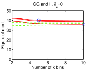
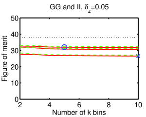
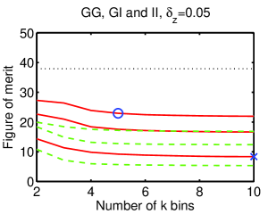
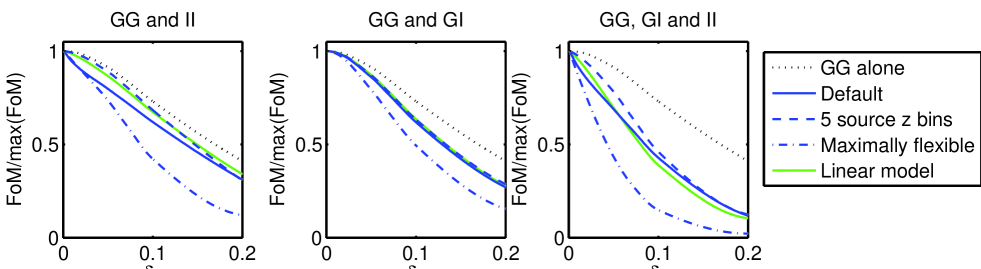
First we consider the effect on the FoM of unknown intrinsic alignment terms in the case of perfect photometric redshifts (). If no II or GI terms are included for our fiducial survey. The upper left panel of Fig. 5 shows that when the II term is included we can actually get an increase in FoM if sufficiently little freedom is given in the intrinsic alignment model! This is because the II angular power spectra (Eq. 5) do depend on cosmology even though we have fixed to be independent of cosmology. Because we have here assumed perfect photometric redshifts then the autocorrelation power spectra measure very well the II angular power spectra separately from the GG angular power spectra. Features in the II angular power spectra subtend different angular scales on the sky and thus constrain cosmology through the standard ruler effect. The size of this effect will depend on the fiducial model used for example, if it is a power law with wavenumber then it would not help to constrain cosmology. This constraint weakens as more free parameters are used in the II power spectra. Adding more bins in wavenumber (-axis of panel) and redshift (upper to lower lines) both degrade the constraints by a similar but small amount.
The lower left panel of Fig. 5 shows that in practice even if has few free parameters it will not help to constrain cosmology better than if intrinsic alignments were negligible. This is because with realistic photometric redshifts it is not possible to adequately disentangle the GG and II contributions to the shear power spectra. However the amount of degradation is still relatively small and flat with increasing number of bins in wavenumber.
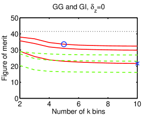
The upper and lower middle panels of Fig. 5 show the result of marginalising over an unknown GI power spectrum in the absence of any II contribution. The degradation is more severe than for the case with II alone. We attribute this to the greater similarity between GG and GI angular power spectra (e.g. Fig 3). Therefore it is more difficult to disentangle the two contributions. Again, the degradation is most sensitive to the number of redshift bins . For the most flexible model we consider the degradation is about a factor of two independent of the photometric redshift error.
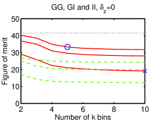
Including both II and GI terms at the same time degrades the dark energy constraints yet further. With zero photometric redshift errors the GG+II result is essentially the same as the GG alone result. We note that also the result for GG+GI+II is almost the same as that for GG+GI. Thus the II parameters are fitted adequately, presumably using the information from the autocorrelation power spectra. However when more realistic photometric redshifts are considered we see that the II term does cause a degradation.
It is not physical to allow complete freedom in the intrinsic alignment power spectra. There are various physical processes that cause the power spectra to vary with scale and redshift. For example, the processes that tidally align galaxies with neigboring mass clumps (Hirata and Seljak, 2004) may evolve differently to those which align galaxy light and mass, and thus cause GI correlations (Bridle and Abdalla, 2007). It is very unlikely that there are so many physical processes that the power spectra could, for example, oscillate in the redshift direction 5 times between redshift 3 and 0. Similarly it is hard to think of physical mechanisms to cause ten changes in power law slope in the k direction. Our most flexible model has 52 free parameters for the GI underlying power spectrum and the same again for the II power spectrum. Considering this large number of free parameters it is perhaps surprising that the cosmological parameter constraints are not weakened still further. We take as our default model for the remainder of the paper , , which means we have freedom in 5 bins in the wavenumber direction as illustrated in Fig. 4 and the same power law in the redshift direction for each wavenumber bin. We also show some results from our maximally free model with and .
We repeat all the calculations using the linear matter power spectrum in the linear alignment model (Eq. 6 and Eq. 11), shown by the dashed lines in Fig. 5. We see that most of our results are qualitatively similar, although the FoMs are generally lower. We attribute this to the difficulty of constraining the parameters of the intrinsic alignment model from a lower signal (the linear matter power spectrum is lower than the non-linear matter power spectrum on small scales).
4. Photometric Redshift Quality
Photometric redshifts exploit spectral features to use images taken with broad wavelength filters to estimate redshifts and hence make a three dimensional map of the universe. We follow Amara and Refregier (2006) in using two parameters to describe photometric redshift quality. The first quantifies nearby scatter about the true spectroscopic redshift , where is the width of the Gaussian contribution centered on the true redshift. The second allows a fraction of catastrophic outliers to exist at a distance from the central Gaussian distribution. Throughout we set for simplicity. See the appendix of Amara and Refregier (2006) and Abdalla et al. (2007) for more details.
4.1. Number of redshift bins
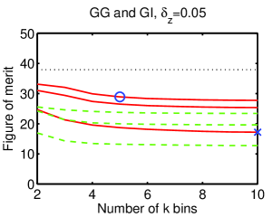
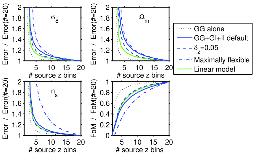
We first consider the effect of the number of redshift bins used for the source galaxies on cosmological parameter uncertainties. For this investigation we assume perfect photometric redshifts by default. It has been noted by several authors for the shear signal (GG) alone (e.g. Hu (1999); Simon et al. (2004); Ma et al. (2006); Amara and Refregier (2006); Jain et al. (2007)) that although a small amount of tomographic information greatly improves parameter constraints, continuing to subdivide into further redshift bins beyond does not significantly reduce uncertainties further. This can be seen by the dotted line in Fig. 6. Using about 3 redshift bins brings parameter constraints to within about 20 per cent of the best obtainable.
However on including intrinsic alignments we expect to need more information to constrain more parameters. The amount that the constraints on cosmological parameters are weakened will depend on the number of free parameters in our intrinsic alignment modeling. We start by considering 5 bins in wavenumber plus an overall amplitude and redshift power law (7 parameters for each of II and GI). This corresponds to the circles marked in Fig. 5.
The solid line in Fig. 6 shows that to reduce uncertainties to 20 per cent of the minimum we now need about 6, 7 or 5 redshift bins for , and respectively. We need 10 redshift bins to bring the FoM to 80 per cent of its maximum value. The maximum number of redshift bins we have used is 20, but if we were to use more then the numbers of redshift bins required would be larger. Thus about twice as many (or more) redshift bins are required to extract the best possible results from the data for the parameters , and twice as many bins are required, whereas three times as many are needed for the FoM.
For the above we have assumed perfect photometric redshifts. We now consider a photometric redshift error of . Therefore at the median survey redshift the photometric redshift uncertainty is so there is potential for effectively about 20 redshift bins between . The non-zero photometric redshift error has negligible effect on the lensing alone (GG) curve and so we do not plot it. This is in keeping with the fact that a small number of redshift bins are sufficient to extract most of the information. For the cases in which we have marginalized over intrinsic alignment parameters then the non-zero photometric redshift error simply causes the curves to converge to the best possible FoM at a smaller number of redshift bins. This is because the best possible FoM is limited by the photometric redshift quality, and in effect sets a maximum number of redshift bins, thus increasing the best obtainable parameter uncertainty. As an example we show the result for our default intrinsic alignment model by the dashed lines in Fig. 6.
We return to perfect photometric redshifts to check the effect of our choice of parametrization of the intrinsic alignments. We considered reducing the number of wavenumber bins from 5 to 2 (while keeping just one redshift bin). This made negligible difference compared to our default parametrization (solid line) so we do not show it in the Figure. We next switch to our maximally flexible intrinsic alignment model (, ). The dot-dashed lines in Fig. 6 show how much the required number of redshift bins is increased. We now need 8, 9, 10, 12 bins to reach 20 per cent of the best uncertainty for , , and the FoM respectively, a factor of 3 or 4 more than that required by lensing alone.
We repeated all the above results using a different fiducial model (, ) and found that these relative results changed very little, even though the parameter constraints are tighter for this model with a larger signal. We see that the results are similar if using the linear matter power spectrum in the linear alignment model (light solid line in Fig. 6). The photometric redshift requirements are less stringent but this is partly because the constraints are already more degraded (see Fig. 5).
4.2. Photometric redshift error
Although it is qualitatively helpful to think about the number of photometric redshift bins, in practice we will have a limited photometric redshift accuracy and will use as many redshift bins as computationally possible (or a fully three dimensional analysis Heavens et al. (2006)). We therefore repackage our results in terms of the photometric redshift accuracy parameter . We also investigate the relative importance of the inclusion of the II and GI terms, but focus in on the FoM for dark energy.
The photometric redshift uncertainties expected from future surveys depend critically on the number of observing filters. Using real data with approximately four optical observing bands a typical scatter is about to (Csabai et al., 2003; Collister and Lahav, 2004; Padmanabhan et al., 2005; Ilbert et al., 2006; Abdalla et al., 2007).
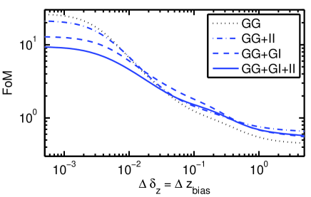
Considering the lensing terms alone, we find again the usual result that the constraints are not very sensitive to photometric redshift quality (dotted lines in Fig. 7).
Ignoring intrinsic-shear correlations for now, we see in the left hand panel of Fig. 7 that the II term always prefers better photometric redshifts, when the number of redshift bins is large i.e. the solid line does not flatten at low . This makes sense because the correlation length for intrinsic alignments ( Mpc) is small compared to the photometric redshift errors. For instance, at , a comoving distance of 10 Mpc corresponds to a , and a is 125 Mpc.
Some works propose to remove the II contamination by removing physically close pairs (King and Schneider, 2002; Heymans and Heavens, 2003; Takada and White, 2004), instead of marginalising over a model. It is clear that for this technique the quality of the photometric redshifts is paramount if a large number of pairs are not to be rejected.
To take only a 20 per cent reduction in the FoM (relative to the best possible) the lensing alone allow , whereas to remove the II term of intrinsic alignments requires twice the precision (). The left hand panel of Fig. 7 shows that this result is relatively independent of the model used for intrinsic alignments (solid and dot-dashed lines are similar at low ). A very flexible model does very badly for poor photometric redshift information. As expected, the number of redshift bins is most important at high photometric redshift accuracy (low ).
Considering just the GI term (and ignoring the II), the middle panel of Fig. 7 shows roughly similar results to the left hand panel (II but no GI). The curves are flatter at high photometric redshift accuracy (smaller ) which can be explained by the inclusion of the broad lensing kernel in the GI redshift dependence. The number of tomographic redshift bins is not crucial for removing the GI term from the GG (the solid, 20 bins, and dashed, 5 bins, lines are very similar). However the photometric redshift quality is still important. A twenty per cent reduction in relative FoM requires approximately 30 per cent smaller redshift uncertainties than if no intrinsic alignments are considered.
Including both the GI and II terms gives a bigger hit on parameter accuracy than only one term alone. This is not surprising since we have significantly increased the number of free parameters, without adding any more data. The results look qualitatively like those for GG+II alone, but place even more stringent constraints on photometric redshift quality. To obtain 80 per cent of the best possible FoM, the photometric redshift errors now need to be a factor of 3 to 4 better than if considering lensing alone, depending on the number of parameters considered in the intrinsic alignment analysis.
Slicing in the opposite direction, if the photometric redshift quality is about , the lensing constraints are degraded by only 10 per cent, relative to that for perfect photometric redshifts. Whereas additionally considering II, GI or GI+II terms degrades the FoM by 25, 20 and per cent, relative to that with perfect photometric redshifts.
For all the combinations, we find the results are not very sensitive to the number of wavenumber bins used in the II and GI parameterization (n=5 and n=20 bins give essentially the same curves, whether m=1 or m=5 redshift bins for the II and GI parametrization are used). The light solid line in Fig. 7 shows the result using the linear matter power spectrum in the linear alignment model. Again we see that the requirements are similar but slightly less stringent. We repeated the default calculations using an outlier fraction but find the results to be negligibly different, i.e. all the FoMs are degraded by the same factor on changing .
We repeated the calculations shown in Fig. 7 but varying instead of on the x-axis of the figure. However we found that there was little difference between the different lines. All dropped to 80 per cent of the maximum FoM at . When intrinsic alignments (GG+GI+II) were included needed to be 10 per cent smaller than when intrinsic alignments were assumed to be negligible (GG alone). When fewer redshift bins were used the requirements on were weaker (5 redshift bins instead of 20 allowed the required to increase by 30 per cent). This shows that it is useful to carry out an analysis with more than 5 redshift bins to make maximum use of the information available.
5. Effect of Priors

So far we have placed very wide priors on the parameters of the intrinsic alignment model, and assumed that the photometric redshift distributions are perfectly known. We now consider narrowing the priors on intrinsic alignment parameters and allowing uncertainty in the lensed galaxy redshift distributions. Throughout the below we place the lensed galaxies in 20 photometric redshift bins, assume default photometric redshift parameters , and default intrinsic alignment model with 5 bins in wavenumber, and the same power law in redshift for each wavenumber (, ).
5.1. Priors on Intrinsic Alignment Model
We now investigate the impact of tighter constraints on the intrinsic alignment modeling, that could come from observations like those of Mandelbaum et al. (2006); Hirata et al. (2007) or advances in theoretical predictions (e.g. Heymans et al., 2006b; van den Bosch et al., 2002). We have previously been using a very wide Gaussian prior on each bin coefficient of width for numerical stability. Fig. 8 shows how the FoM increases as this value is decreased. We can see that the wide prior we used for the earlier sections was sufficiently wide that the self-calibration regime was reached. We also see that if the priors on the IA model are sufficiently tight then the constraints on cosmology (GG+GI+II) are tighter than if intrinsic alignments were negligible (GG).
As in Fig 5, GG+GI gives a lower FoM than GG+II. In addition the transition to the self-calibration regime occurs at smaller for GG+GI than for GG+II. This means that more precise information is required to alleviate the cosmological parameter degradation, compared to GG+II. The exact transition to self-calibration will in general depend on the number of parameters being fitted, however for our default model with 7 parameters for each of II and GI, priors on the perturbing parameters need to be less than 10 per cent to help improve cosmological parameters constraints. We repeated the calculation keeping the overall amplitude and power law parameters fixed but the qualitative picture remains the same.
5.2. Priors on redshift distributions
In practice the redshift distributions of the lensed galaxies cannot be known perfectly because we only have imperfect photometric redshifts. So far we have dealt with the accuracy properties of each single photometric redshift estimate, in terms of a scatter parameter and a catastrophic outlier parameter. For cosmic shear it is generally much more important to have accurate knowledge of these parameters than for these parameters to be small. It is difficult to know the values of these parameters accurately since they depend on uncertain modeling of galaxy formation (Abdalla et al., 2007) and/or large test samples for which spectroscopic redshifts are known.
Here, we discuss our knowledge of these parameters by considering our uncertainty on them, and place Gaussian priors on their values. This follows previous work (Huterer et al., 2006; Ma et al., 2006; Jain et al., 2007; Amara and Refregier, 2006), which has also discussed the numbers of spectroscopic redshifts needed to obtain these priors. We revert back to wide priors on the intrinsic alignment parameters .
We divide the redshift range up into 30 photometric redshift prior bins such that an equal number of galaxies fall into each bin. We apply a shift of to all the spectroscopic redshifts in bin number . We assign the scatter for bin to be . We then allow these 30 parameters to vary in the Fisher matrix and apply priors of width and which are the same for every photometric redshift prior bin. We then create the joint probability distribution and make cuts in photometric redshift space, as before.
This is the same as in Ma et al. (2006) except we vary instead of and using binning with equal numbers of galaxies in each bin instead of even spacing in redshift. The broad results are similar but more accentuated when we switch to the Ma et al. (2006) method.
The results in Fig. 9 show that in terms of absolute FoM, tighter priors are required when intrinsic alignments are considered, if we are to obtain the same FoM as in their absence. For example, to obtain an FoM of 10 extremely tight priors are required if considering GG+GI+II, whereas a wider prior could be used if intrinsic alignments did not exist (GG). However, if we are considering the relative figure of merit then the results are reversed. To obtain 80 per cent of the best possible FoM, the presence of intrinsic alignments allows us to loosen our requirements on the priors, and thus allow smaller spectroscopic redshift training sets. Note that this is because the best possible FoM is lower when we take into account intrinsic alignments.
If we had particularly poor prior knowledge of photometric redshift properties, then the existence of intrinsic alignments actually helps to calibrate the uncertain parameters. This is particularly true for the intrinsic-intrinsic term. Note that this all assumes our default photometric redshift fiducial model in which and . Therefore if photometric redshifts were good, but we did not know it, then intrinsic alignments would help.
For our example with 30 photometric redshift parameter bins the FoM with intrinsic alignments included (GG+GI+II) is better than that if intrinsic alignments did not exist for . However, a considerable fraction of the FoM has been lost by this stage so we hope not to be in this regime. Following Ma et al. (2006) we would already have a prior tighter than this if we had a number spectroscopic redshifts in each photometric redshift parameter bin. It is likely we will already have more spectroscopic redshifts than this, but perhaps this feature might become useful for very deep surveys, for which spectroscopy will be harder to obtain, or as a cross-check.
6. Conclusions
We have compared our fiducial model to current observations and an alternative model and found it to be in good agreement. We use the linear alignment model as our base, and investigate inserting the non-linear matter power spectrum, as a way of taking into account small scale correlations (as suggested in Hirata et al. (2007)). We find that this matches better to the HRH* model for intrinsic-intrinsic (II) alignments, and matches better to the GI detections of Mandelbaum et al. (2006); Hirata et al. (2007).
We allow this model freedom as a function of scale and redshift since we will not know the intrinsic alignment contributions perfectly in time for future dark energy surveys, due to the dependence on baryonic physics. We choose as our baseline model one which has five free parameters as a function of scale, and the same power law function of redshift for each scale. We allow the option of adding more redshift variation, and more or less parameters as a function of wavenumber. We assume the II and GI perturbations about the linear alignment model are independent of each other.
We find that if little freedom is given to the intrinsic alignment modeling then the constraints on dark energy parameters can actually be very slightly improved, relative to those obtained if intrinsic alignments do not exist. Essentially the intrinsic alignments are providing another cosmological probe.
The shear-intrinsic correlations are more subtle since they contain the lensing efficiency function. It seems plausible that cross correlations between a given redshift bin and the various other redshift bins will allow simultaneous constraints on the GI term and cosmology. This is not so dissimilar to the lensing geometric test (Jain and Taylor, 2003; Hu and Jain, 2004; Bernstein and Jain, 2004), in which the mass of halos is jointly constrained with cosmology due to the dependence of the shear signal with redshift. However, on allowing realistic freedom in the intrinsic alignment modeling and using more realistic photometric redshift uncertainties the potential is lost, and dark energy constraints are degraded by about 50 per cent.
We show how the number of source galaxy redshift bins affects cosmological parameter constraints with and without intrinsic alignments. We find that on considering intrinsic alignments the number of redshift bins must be doubled or tripled to obtain the full information available.
We investigate in more detail the effect of photometric redshift quality on constraints. We consider how constraints are degraded with respect to the case in which perfect photometric redshifts are available. We confirm that intrinsic alignments put tighter constraints on photometric redshift quality than lensing alone. We find roughly equal contributions from each of the II and GI terms. The photometric redshift error required is approximately three times smaller that using lensing alone, to extract the same fraction of the available information. It would therefore be most unwise to plan future gravitational lensing experiments to capitalize on the result that lensing does not require precise redshift information. The color tomography method of Jain et al. (2007) could likely still be applied if enough observing bands were used.
A significant catastrophic outlier fraction would be bad news for methods for removing the intrinsic-intrinsic correlations by excluding pairs of galaxies from the analysis. Statistically it may be known that there is a ten per cent chance the true redshift is far from that measured. Deciding whether or not to remove the pair is then more unclear, and contamination will leak in. Modeling the intrinsic-intrinsic correlations means that statistical information on the redshift distribution is sufficient i.e. we can use the number as a function of redshift for each bin rather than a precise redshift of each galaxy. However we do need to use an intrinsic alignment model that can encapsulate the true intrinsic alignment contribution.
Mandelbaum et al. (2006) suggested excluding brightest cluster galaxies (BCGs; which often pass the cuts used to select luminous red galaxies, LRGs) from samples used to measure cosmic shear, in order to minimize the intrinsic terms. However, these galaxies do have smaller photometric redshift errors and hence would be useful to include in 3-D lensing studies, as well as in the constraint of cosmological parameters that we have considered here. Perhaps simultaneously fitting for the intrinsic terms as well as for the cosmic shear signal as a function of galaxy type (plus relative redshift and scale), rather than excluding BCGs would be possible. In this paper we have ignored the fact that the intrinsic alignment parameters depend on galaxy type.
Obtaining additional information on the intrinsic alignments from other sources would be extremely valuable, since the degradation of cosmological parameter constraints is large on using a very flexible model for intrinsic alignments. This could come from better numerical simulations or from observations of the galaxy-shear and galaxy-galaxy cross correlation functions such as those by Mandelbaum et al. (2006); Hirata et al. (2007) or as suggested by Hu and Jain (2004). We find that priors of around 10 per cent would be helpful.
Cosmic shear produces only E-mode (curl-free) distortions, except on sub-arcminute scales where source clustering induces a B-mode signal (Schneider et al., 2002). The presence of B-mode distortions would indicate that residual systematics are present, either from incomplete correction of galaxy ellipticities for distortions (associated with the atmosphere or telescope) or from intrinsic galaxy alignments. The magnitudes of the B-mode power spectra of II and GI are highly model dependent - thus, if one can be sure that the data have been accurately corrected for other systematics, this signal will place stringent constaints on which physical models of intrinsic alignment are supported by the data.
To summarise our findings:
-
•
When constraining the dark energy equation of state using a cosmic shear survey, it is essential to account for intrinsic-intrinsic galaxy alignments (II correlations) and the cross-term between intrinsic ellipticity and cosmic shear (GI correlations). Neglecting these correlations biases the dark energy equation of state by 50%.
-
•
We considered a range of flexibility in the intrinsic alignment modelling and found a wide variation in the impact on the degradation in the dark energy figure of merit. It will be necessary for future observational and theoretical studies to inform this choice when making future dark energy constraints.
-
•
In general when II and GI correlations are accounted for in cosmological parameter estimation, the number of tomographic redshift bins must be a factor of at least two more than if only lensing correlations are present, to obtain 80% of the available information.
-
•
Concerning the dark energy figure of merit, the presence of II and GI correlations places a more stringent requirement on the accuracy of photometric redshifts - a factor of - compared with the case where only cosmic shear is present.
Acknowledgements
We thank Gary Bernstein, Tom Kitching, Masahiro Takada, Filipe Abdalla, Chris Blake, Patrick Simon, Adam Amara, Alexandre Refregier, Antony Lewis, Bhuvnesh Jain and Ofer Lahav for helpful discussions. SLB and LJK acknowledge support from Royal Society University Research Fellowships.
References
- Blandford et al. (1991) R. D. Blandford, A. B. Saust, T. G. Brainerd, and J. V. Villumsen, MNRAS 251, 600 (1991).
- Miralda-Escude (1991) J. Miralda-Escude, ApJ 370, 1 (1991).
- Kaiser (1992) N. Kaiser, ApJ 388, 272 (1992).
- Bacon et al. (2000) D. J. Bacon, A. R. Refregier, and R. S. Ellis, MNRAS 318, 625 (2000), astro-ph/0003008.
- Kaiser et al. (2000) N. Kaiser, G. Wilson, and G. A. Luppino, ArXiv Astrophysics e-prints (2000), astro-ph/0003338.
- Van Waerbeke et al. (2000) L. Van Waerbeke, Y. Mellier, T. Erben, J. C. Cuillandre, F. Bernardeau, R. Maoli, E. Bertin, H. J. Mc Cracken, O. Le Fèvre, B. Fort, et al., A&A 358, 30 (2000), astro-ph/0002500.
- Wittman et al. (2000) D. M. Wittman, J. A. Tyson, D. Kirkman, I. Dell’Antonio, and G. Bernstein, Nature 405, 143 (2000), astro-ph/0003014.
- Hu (2002) W. Hu, Phys. Rev. D 65, 023003 (2002), astro-ph/0108090.
- Crittenden et al. (2001) R. G. Crittenden, P. Natarajan, U.-L. Pen, and T. Theuns, ApJ 559, 552 (2001), astro-ph/0009052.
- Hirata and Seljak (2004) C. M. Hirata and U. Seljak, Phys. Rev. D 70, 063526 (2004), astro-ph/0406275.
- Croft and Metzler (2000) R. A. C. Croft and C. A. Metzler, ApJ 545, 561 (2000), astro-ph/0005384.
- Heavens et al. (2000a) A. Heavens, A. Refregier, and C. Heymans, MNRAS 319, 649 (2000a), astro-ph/0005269.
- Mackey et al. (2002) J. Mackey, M. White, and M. Kamionkowski, MNRAS 332, 788 (2002), astro-ph/0106364.
- Jing (2002) Y. P. Jing, MNRAS 335, L89 (2002), astro-ph/0206098.
- Hirata et al. (2004) C. M. Hirata, R. Mandelbaum, U. Seljak, J. Guzik, N. Padmanabhan, C. Blake, J. Brinkmann, T. Budávari, A. Connolly, I. Csabai, et al., MNRAS 353, 529 (2004), astro-ph/0403255.
- Bridle and Abdalla (2007) S. Bridle and F. B. Abdalla, ApJ 655, L1 (2007), astro-ph/0608002.
- Brown et al. (2003) M. Brown, A. N. Taylor, N. C. Hambly, and S. Dye, MNRAS 333, 501 (2002).
- Heymans et al. (2004a) C. Heymans, M. Brown, A. Heavens, K. Meisenheimer, A. Taylor, and C. Wolf, MNRAS 347, 895 (2004a), astro-ph/0310174.
- King and Schneider (2002) L. King and P. Schneider, A&A 396, 411 (2002), astro-ph/0208256.
- Heymans and Heavens (2003) C. Heymans and A. Heavens, MNRAS 339, 711 (2003), astro-ph/0208220.
- Takada and White (2004) M. Takada and M. White, ApJ 601, L1 (2004), astro-ph/0311104.
- King and Schneider (2003) L. J. King and P. Schneider, A&A 398, 23 (2003), astro-ph/0209474.
- Hirata et al. (2007) C. M. Hirata, R. Mandelbaum, M. Ishak, U. Seljak, R. Nichol, K. A. Pimbblet, N. P. Ross, and D. Wake, ArXiv Astrophysics e-prints (2007), astro-ph/0701671.
- Heymans et al. (2006a) C. Heymans, M. White, A. Heavens, C. Vale, and L. van Waerbeke, MNRAS 371, 750 (2006a), astro-ph/0604001.
- King (2005) L. J. King, A&A 441, 47 (2005), astro-ph/0506441.
- Mandelbaum et al. (2006) R. Mandelbaum, C. M. Hirata, M. Ishak, U. Seljak, and J. Brinkmann, MNRAS 367, 611 (2006), astro-ph/0509026.
- Peacock and Dodds (1996) J. A. Peacock and S. J. Dodds, MNRAS 280, L19 (1996), astro-ph/9603031.
- Ma (1996) C.-P. Ma, Astrophys. J. 471, 13 (1996), astro-ph/9605198.
- Catelan et al. (2001) P. Catelan, M. Kamionkowski, and R. D. Blandford, MNRAS 320, L7 (2001), astro-ph/0005470.
- Heavens et al. (2000b) A. Heavens, A. Refregier, and C. Heymans, MNRAS 319, 649 (2000b), astro-ph/0005269.
- Heymans et al. (2004b) C. Heymans, M. Brown, A. Heavens, K. Meisenheimer, A. Taylor, and C. Wolf, MNRAS 347, 895 (2004b), astro-ph/0310174.
- Spergel (2006) D. N. e. a. Spergel, ArXiv Astrophysics e-prints (2006), astro-ph/0603449.
- Chevallier and Polarski (2001) M. Chevallier and D. Polarski, International Journal of Modern Physics D 10, 213 (2001), gr-qc/0009008.
- Linder (2003) E. V. Linder, Physical Review Letters 90, 091301 (2003), astro-ph/0208512.
- Amara and Refregier (2006) A. Amara and A. Refregier, ArXiv Astrophysics e-prints (2006), astro-ph/0610127.
- Smail et al. (1994) I. Smail, R. S. Ellis, and M. J. Fitchett, MNRAS 270, 245 (1994), astro-ph/9402048.
- Huterer et al. (2006) D. Huterer, M. Takada, G. Bernstein, and B. Jain, MNRAS 366, 101 (2006), astro-ph/0506030.
- Albrecht et al. (2006) A. Albrecht, G. Bernstein, R. Cahn, W. L. Freedman, J. Hewitt, W. Hu, J. Huth, M. Kamionkowski, E. W. Kolb, L. Knox, et al., ArXiv Astrophysics e-prints (2006), astro-ph/0609591.
- Takada and Jain (2004) M. Takada and B. Jain, MNRAS 348, 897 (2004), astro-ph/0310125.
- Abdalla et al. (2007) F. Abdalla, A. Amara, P. Capak, E. Cypriano, O. Lahav, and J. Rhodes, MNRASsubmitted (2007).
- Hu (1999) W. Hu, ApJ 522, L21 (1999), astro-ph/9904153.
- Simon et al. (2004) P. Simon, L. J. King, and P. Schneider, A&A 417, 873 (2004), astro-ph/0309032.
- Ma et al. (2006) Z. Ma, W. Hu, and D. Huterer, ApJ 636, 21 (2006), astro-ph/0506614.
- Jain et al. (2007) B. Jain, A. Connolly, and M. Takada, Journal of Cosmology and Astro-Particle Physics 3, 13 (2007), astro-ph/0609338.
- Heavens et al. (2006) A. F. Heavens, T. D. Kitching, and A. N. Taylor, Mon. Not. Roy. Astron. Soc. 373, 105 (2006), astro-ph/0606568.
- Csabai et al. (2003) I. Csabai et al. (SDSS), Astron. J. 125, 580 (2003), astro-ph/0211080.
- Collister and Lahav (2004) A. A. Collister and O. Lahav, Publ. Astron. Soc. Pac. 16, 345 (2004), astro-ph/0311058.
- Padmanabhan et al. (2005) N. Padmanabhan et al. (SDSS), Mon. Not. Roy. Astron. Soc. 359, 237 (2005), astro-ph/0407594.
- Ilbert et al. (2006) O. Ilbert et al., A&A 457, 841 (2006), astro-ph/0603217.
- Heymans et al. (2006b) C. Heymans, M. White, A. Heavens, C. Vale, and L. van Waerbeke, MNRAS 371, 750 (2006b), astro-ph/0604001.
- van den Bosch et al. (2002) F. C. van den Bosch, T. Abel, R. A. C. Croft, L. Hernquist, and S. D. M. White, Astrophys. J. 576, 21 (2002), astro-ph/0201095.
- Jain and Taylor (2003) B. Jain and A. Taylor, Physical Review Letters 91, 141302 (2003), astro-ph/0306046.
- Hu and Jain (2004) W. Hu and B. Jain, Phys. Rev. D 70, 043009 (2004), astro-ph/0312395.
- Bernstein and Jain (2004) G. Bernstein and B. Jain, ApJ 600, 17 (2004), astro-ph/0309332.
- Schneider et al. (2002) P. Schneider, L. van Waerbeke, and Y. Mellier, A&A 389, 729 (2002), arXiv:astro-ph/0112441.