Is Modified Gravity Required by Observations?
An Empirical Consistency Test of Dark Energy Models

Abstract

We apply the technique of parameter splitting to existing cosmological data sets, to check for a generic failure of dark energy models. Given a dark energy parameter, such as the energy density $\Omega_{\Lambda}$ or equation of state $w$, we split it into two meta–parameters with one controlling geometrical distances, and the other controlling the growth of structure. Observational data spanning Type Ia supernovae, the cosmic microwave background (CMB), galaxy clustering, and weak gravitational lensing statistics are fit without requiring the two meta–parameters to be equal. This technique checks for inconsistency between different data sets, as well as for internal inconsistency within any one data set (e.g., CMB or lensing statistics) that is sensitive to both geometry and growth. We find that the cosmological constant model is consistent with current data. Theories of modified gravity generally predict a relation between growth and geometry that is different from that of general relativity. Parameter splitting can be viewed as a crude way to parametrize the space of such theories. Our analysis of current data already appears to put sharp limits on these theories: assuming a flat universe, current data constrain the difference $\Delta\Omega_{\Lambda}=\Omega_{\Lambda}{\rm(geom)}-\Omega_{\Lambda}{\rm(grow)}$ to be $-0.0044^{+0.0058+0.0108}_{-0.0057-0.0119}$ ($68\%$ and $95\%$ C.L. respectively); allowing the equation of state $w$ to vary, the difference $\Delta w=w{\rm(geom)}-w{\rm(grow)}$ is constrained to be $0.37^{+0.37+1.09}_{-0.36-0.53}$. Interestingly, the region $w{\rm(grow)}>w{\rm(geom)}$, which should be generically favored by theories that slow structure formation relative to general relativity, is quite restricted by data already. We find $w{\rm(grow)}<-0.80$ at $2\sigma$. As an example, the best–fit flat Dvali–Gabadadze–Porrati (DGP) model approximated by our parametrization lies beyond the $3\sigma$ contour for constraints from all the data sets.

I Introduction

Observations of distant supernovae (SNe), galaxies, clusters of galaxies, and the cosmic microwave background (CMB) have shown that, surprisingly, the cosmic expansion is accelerating. This reveals that fundamentally new physics is missing from our understanding of the universe DETF .

The cosmic acceleration may arise either from “dark energy,” a mysterious yet presently dominant component of the total energy density, or from “modified gravity,” a modification of general relativity (GR) on large scales. The first case includes, for example, Einstein’s cosmological constant or quintessence, a dynamical scalar field Quint . The second case includes modifications of four–dimensional GR due to the presence of extra dimensions, scalar–tensor theories, and others DGP ; MG ; others .

Current efforts focus, within the dark energy paradigm, on improving the constraints on the dark energy density $\Omega_{\rm DE}$, its equation of state (EOS) $w\equiv P/\rho$ and its time evolution $dw/da$ (where $a$ is the scale factor), by using observational data that bear on geometrical distances and the growth of structure. As first emphasized by LSS and subsequently discussed by many others many , GR predicts a definite relation between geometrical distances and growth which is generically violated by modified theories of gravity. To the extent current data (that are sensitive to different combinations of geometry and growth) yield consistent dark energy constraints, one can interpret this as a confirmation of the dark energy + GR framework. The simplest dark energy model, the cosmological constant, has passed this kind of consistency test so far WMAP .

In this paper, we sharpen the consistency test. Our method goes by the name of “parameter splitting” as proposed by ZHS ; CK . Let us illustrate the technique using the cosmological constant ($\Lambda$)–cold dark matter (CDM) model. Instead of fitting the suite of observational data with a single cosmological constant density parameter $\Omega_{\Lambda}$ (in addition to, of course, other non–dark energy parameters), we fit them with two parameters $\Omega_{\Lambda}{\rm(geom)}$ and $\Omega_{\Lambda}{\rm(grow)}$: one determining the geometrical distances, and the other controlling the growth of structure. The conventional approach is to assume the two parameters are equal. Here, they are allowed to vary separately. We employ the Markov chain Monte Carlo (MCMC) technique MCMC to derive the marginalized constraints on both parameters. If the $\Lambda$CDM model is correct, these two parameters should agree within their uncertainties. This technique of splitting a conventional parameter into two “meta–parameters” can of course be applied to any other parameter. In this paper, we will consider the splitting of both $\Omega_{\Lambda}$ and $w$.

It is important to emphasize that parameter splitting checks for consistency not only between different data sets, but also for internal consistency within any single data set that is sensitive to both geometry and growth. In some sense, the conventional approach of obtaining constraints on, e.g., $\Omega_{\Lambda}$ separately from SNe, CMB, lensing and so on, and checking that they are consistent, is itself a simple form of parameter splitting, i.e., splitting $\Omega_{\Lambda}$ into $\Omega_{\Lambda}$(SNe), $\Omega_{\Lambda}$(CMB), $\Omega_{\Lambda}$(lensing), etc. The parameter splitting that we employ here represents a more stringent, and theoretically better motivated, consistency test. It is also useful to note that there is a wide variety of modified gravity theories. Our splitting of $\Omega_{\Lambda}$ and $w$ can be thought of as a crude way to parametrize the space of such theories. For instance, in the Dvali–Gabadadze–Porrati (DGP) theory DGP where gravity becomes weaker on large scales, structure growth is slowed and therefore one expects qualitatively $w{\rm(grow)}>w{\rm(geom)}$ LSS ; footnote1 .

We caution that should an inconsistency be discovered via parameter splitting, modified gravity is not the only possible interpretation. Systematic problems with the data, as well as complications in the dark energy model (such as a time varying $w$ or nontrivial dark energy clustering kunz ), are also possible. Additional parameters need to be introduced to check for the latter case. Parameter splitting can be applied to the new parameters as appropriate.

II Geometry

All geometrical distances in cosmology, such as the luminosity or angular diameter distance, are related to the radial comoving distance

$$\chi(z)=\int^{z}_{0}\frac{dz^{\prime}}{H(z^{\prime})},$$ (1)

setting the speed of light $c=1$. The Hubble parameter $H$ as a function of redshift $z$, i.e., the expansion history, can be parametrized as follows:

$$\frac{H^{2}(z)}{H^{2}_{0}}=\Omega_{m}(1+z)^{3}+\Omega_{r}(1+z)^{4}+\Omega_{\rm DE}(1+z)^{3(1+w)},$$ (2)

where $H_{0}=100h$ km s^-1Mpc^-1 is the Hubble constant today. Throughout this paper, we assume that the universe is spatially flat, the dark energy has a constant EOS parameter $w$ and all three species of neutrinos are massless. $\Omega_{r}$ is the radiation density today, in units of the critical density, including photons and massless neutrinos; $\Omega_{\rm DE}$ is the present dark energy density, denoted as $\Omega_{\Lambda}$ for the cosmological constant model ($w=-1$). Note that for a flat universe, the dimensionless matter density $\Omega_{m}$ can be replaced by $1-\Omega_{r}-\Omega_{\rm DE}$. We will use a superscript “(geom)” to denote the dark energy parameters appearing in the expressions of geometrical distances.

III Growth

Inhomogeneities grow under gravitational instability according to the prevailing structure formation paradigm. The dynamics within the GR framework is described by a set of Boltzmann–Einstein equations well documented in the literature dodelson . In this paper, we use the publicly available code CAMB LCL to evolve these equations. For the purpose of illustrating our method, and purely for this purpose, let us consider the special case of subhorizon matter fluctuations in the late universe. They evolve according to $\ddot{\delta}_{m}+2H\dot{\delta}_{m}=4\pi G\rho_{m}\delta_{m}$, where $\delta_{m}\equiv\delta\rho_{m}/\rho_{m}$ is the matter overdensity, $\rho_{m}$ is the average matter density, $G$ is the Newton constant and the dots denote proper time derivatives. We ignore the dark energy perturbations here for simplicity. The growth equation can be rewritten as

$$\frac{d^{2}\delta_{m}}{d\ln{a}^{2}}+\left[\frac{d\ln{H}}{d\ln{a}}+2\right]\frac{d\delta_{m}}{d\ln{a}}=\frac{3\Omega_{m}H_{0}^{2}}{2a^{3}H^{2}}\delta_{m},$$ (3)

where $a=1/(1+z)$ is the scale factor. Therefore, the expansion history [Eq. (2)] that determines geometrical distances also determines the growth of structure, in a way that is uniquely predicted by GR.

It is not surprising that, in order to match existing data, viable theories of modified gravity often predict an expansion history (and therefore geometrical distances) that is similar to the one in Eq. (2). Such theories, however, generally predict a relation between expansion history and growth that is different from the one in Eq. (3). Given the wide variety of these theories, and in the absence of a particularly compelling candidate ghosts , a crude way to test for such a possibility is to allow the dark energy parameters to take different values in the growth equation [Eq. (3)] from their values in the expression for distance [Eq. (1)], i.e., parameter splitting. We use a superscript “(grow)” to denote the dark energy parameters characterizing the evolution of inhomogeneities.

Note that one has some freedom in exactly how the parameter splitting is performed. For instance, in Eq. (3), the dark energy parameters show up in two places: the second term on the left hand side of the equation ($d\ln{H}/d\ln{a}$) and the term on the right hand side ($\Omega_{m}/H^{2}$). One could choose to assign all of them to the “growth” category which is what we do, or one could assign some to the “geometry” category and the others to the “growth” category. Ultimately, there are many possible consistency tests, and here we have chosen to perform one that is particularly simple to implement, i.e., assigning all dark energy parameters that enter the fluctuation equations to the “growth” category. It is worth noting that in a lot of modified gravity theories, the equivalent of the Poisson’s equation is often modified without modifying energy–momentum conservation. In that case, one could argue assigning the term on the right hand side of Eq. (3) alone to the “growth” category might make more sense. We hope to investigate this in the future.

The exact Boltzmann–Einstein equations for the evolution of structure, allowing for multiple components, photons, neutrinos and so on, are more complicated than Eq. (3). The same parameter–splitting scheme can nevertheless be applied to the exact equations, which is what we do. This means, for example, the shape of the transfer function, such as the radiation–matter equality peak of the power spectrum, is determined by the growth parameters – recall that the transfer function is completely determined by the dynamics of fluctuation growth. The conversion of a feature, such as the radiation–matter equality length scale to an observed angle, on the other hand, involves the geometry parameters.

IV The Parameter–Splitting Technique

To illustrate how the splitting of dark energy parameters into the “geometry” and “growth” categories is done in our analysis, we start with the weak lensing (WL) observables. There exists a natural division between the two categories for each term involved in the calculation ZHS .

WL surveys measure the aperture mass statistic on different angular scales $\theta$:

$$\langle M^{2}_{\rm ap}(\theta)\rangle=\frac{1}{2\pi}\int\ell d\ell~{}P_{\kappa}(\ell)W^{2}(\ell\theta),$$ (4)

where $W$ is a window function with no dependence on cosmology. $P_{\kappa}(\ell)$ is the convergence power spectrum at the angular wavenumber $\ell$, given by

$$P_{\kappa}(\ell) = \frac{9}{4}\Omega^{2}_{m}H_{0}^{4}\int^{\infty}_{0}dz~{}(1+z)^{2}\left[\frac{d\chi(z)}{dz}\right]\xi^{2}(z)~{}P_{\delta}\left[\frac{\ell}{\chi(z)},z\right],$$

$$\xi(z) = \int^{\infty}_{z}dz^{\prime}~{}n_{\rm gal}(z^{\prime})\left[\frac{\chi(z^{\prime})-\chi(z)}{\chi(z^{\prime})}\right].$$ (5)

Here $P_{\delta}[\ell/\chi,z]$ is the matter power spectrum at wavenumber $k=\ell/\chi$ and redshift $z$, $n_{\rm gal}$ is the normalized redshift distribution of the background galaxies, and we have used Limber’s approximation. We express everything in terms of the redshift $z$, which is an observable of the surveys.

Consider for instance the splitting of $\Omega_{\Lambda}$ for the flat $\Lambda$CDM model. The three–dimensional matter power spectrum $P_{\delta}$ and the mean matter density $\Omega_{m}$ ($=1-\Omega_{\Lambda}$, where the contribution of radiation is neglected at low redshifts) sitting outside the integral both describe the foreground inhomogeneities through which photons travel. Therefore they go into the “growth” category and are calculated using $\Omega_{\Lambda}^{\rm(grow)}$. All $\chi$’s within the integral fall naturally in the “geometry” category. This includes the $\chi$ in the wavenumber $\ell/\chi$, which reflects the conversion between the observed angle and the physical length scale. These geometrical distances are all calculated using $\Omega_{\Lambda}^{\rm(geom)}$. A similar split can be applied to $w$ in the context of the quintessence (Q)–CDM model.

With the WL example in mind, we next consider the CMB. The temperature anisotropy power spectrum is given by

$$C^{TT}_{\ell}=\frac{2}{\pi}\int k^{2}dk~{}P_{\Psi}(k)\left|\frac{\Theta_{\ell}(k,z=0)}{\Psi(k)}\right|^{2},$$ (6)

where $\Psi(k)$ is the primordial metric perturbation (in conformal Newtonian gauge), $P_{\Psi}(k)\propto k^{n_{s}-4}$ is the power spectrum of $\Psi$, and $\Theta_{\ell}$ is given by dodelson

$$\Theta_{\ell}(k,z=0)=\int_{0}^{\infty}dz^{\prime}~{}\tilde{S}_{T}(k,z^{\prime})j_{\ell}[k\chi(z^{\prime})].$$ (7)

where $j_{\ell}$ is the spherical Bessel function and $\tilde{S}_{T}$ denotes some source function. All the complicated dynamics is contained in $\tilde{S}_{T}$. Publicly available Boltzmann codes SM ; LCL can be used to compute $\tilde{S}_{T}$, and therefore $\Theta_{\ell}$, for any given primordial perturbation $\Psi$ ($\Theta_{\ell}/\Psi$ is independent of $\Psi$; see dodelson ).

We perform the geometry–growth split of Eq. (7) as follows footnote2 : $\tilde{S}_{T}$ falls under the “growth” category and the rest (namely $\chi(z^{\prime})$ in the argument of $j_{\ell}$) falls under the “geometry” category footnote3 . The rationale for this particular way of splitting is most transparent when considering the Sachs–Wolfe term SW , where $\tilde{S}_{T}(k,z)$ is well approximated by $\delta_{D}(z-z_{\ast})[\Theta_{0}+\Psi](k,z_{\ast})$. Here $\delta_{D}(z-z_{\ast})$ is the Dirac delta function with $z_{\ast}$ being the redshift of last scattering, and $\Theta_{0}(k,z_{\ast})$ and $\Psi(k,z_{\ast})$ are the temperature monopole and metric perturbations at last scattering. Therefore, the Sachs–Wolfe term is

$$\Theta^{\rm SW}_{\ell}(k,z=0)\simeq\left[\Theta_{0}+\Psi\right](k,z_{\ast})~{}j_{\ell}(k\chi_{\ast}),$$ (8)

and our geometry–growth split is equivalent to using the growth parameters to compute $[\Theta_{0}+\Psi](k,z_{\ast})$ and the geometry parameters to compute $\chi_{\ast}$, the distance to last scattering.

It is straightforward to generalize the above splitting scheme to similar expressions describing the polarization spectrum. In the case of SNe, parameter splitting is trivial since SNe constrain only the geometry parameters. The splitting for galaxy clustering is done as follows. As discussed earlier, the growth (as opposed to geometry) parameters determine the transfer function for the matter power spectrum. On the other hand, to measure the three–dimensional power spectrum of galaxies as a function of comoving spatial scale, one has to adopt a cosmological model in order to convert the observed redshifts and angular separations into comoving distances. This conversion is trivial for low–redshift surveys (involving only $H_{0}$) such as the Two–Degree Field Galaxy Redshift Survey (2dFGRS), but is nontrivial for moderate redshift samples, such as the luminous red galaxies (LRGs) in the Sloan Digital Sky Survey (SDSS). For the LRGs, we follow LRG and include a cosmology–dependent rescaling of the $k$–axes HH . This rescaling is included in the “geometry” category.

V Current Observations

Below we list the four data sets used in our analysis. Many of these, though not all, are included in the CosmoMC package CosmoMC .

V.1 Cosmic Microwave Background

We use (i) the recent Wilkinson Microwave Anisotropy Probe (WMAP) three–year data set WMAP , and (ii) small scale CMB observational data including Arcminute Cosmology Bolometer Array Receiver (ACBAR) ACBAR , Balloon Observations Of Millimetric Extragalactic Radiation and Geophysics (BOOMERanG) Boom and Cosmic Background Imager (CBI) CBI . We modify the Boltzmann code CAMB LCL by splitting the dark energy parameters as described above. We assume adiabatic initial fluctuations, and neglect B–mode polarization and tensor modes.

V.2 Supernovae

We use the SNe data set for the Supernova Legacy Survey (SNLS) analysis described in SNLS .

Figure 1: Joint constraints on $\Omega_{\Lambda}^{\rm(geom)}$ and $\Omega_{\Lambda}^{\rm(grow)}$ in a $\Lambda$CDM model (upper panel) and the normalized likelihood distribution of $\Delta\Omega_{\Lambda}\equiv\Omega_{\Lambda}^{\rm(geom)}-\Omega_{\Lambda}^{\rm(grow)}$ (lower panel). Here the equation of state parameters are fixed as $w^{\rm(geom)}=w^{\rm(grow)}=-1$. The contours and curves show the $68\%$ confidence limits from the marginalized distributions. The thick gray lines show $\Omega_{\Lambda}^{\rm(geom)}=\Omega_{\Lambda}^{\rm(grow)}$. The data sets used are described in the text. Different contours and curves represent constraints from different combinations of the data sets. The smallest contour and the most narrow curve (black solid line) represent constraints from all the data. No significant difference is found and deviations are constrained to $\Delta\Omega_{\Lambda}=-0.0044^{+0.0058+0.0108}_{-0.0057-0.0119}$ ($68\%$ and $95\%$ C.L.).

V.3 Galaxy Clustering

We use data sets from (i) the Two–Degree Field Galaxy Redshift Survey (2dFGRS) 2dF , which probes the galaxy distribution at redshift $z\sim 0.1$ and the power spectrum on scales of $0.022h$ Mpc${}^{-1}<k<0.18h$ Mpc^-1, and (ii) the luminous red galaxies in the Sloan Digital Sky Survey (SDSS) LRG , which are at an effective redshift of $z\sim 0.35$ and cover scales between $0.012h$ Mpc${}^{-1}<k<0.20h$ Mpc^-1. Redshift–space distortions, galaxy biasing and nonlinear clustering footnote4 are dealt with in ways described in 2dF ; LRG .

Figure 2: Variations of CMB temperature power spectra due to different changes of $\Omega_{\Lambda}^{\rm(geom)}$ and $\Omega_{\Lambda}^{\rm(grow)}$ (with all the other cosmological parameters fixed) as illustrated in the inset on the $\Omega_{\Lambda}^{\rm(geom)}$ vs. $\Omega_{\Lambda}^{\rm(grow)}$ plane. The black solid curve corresponds to the black square symbol, which is our best–fit $\Lambda$CDM model with $\Omega_{\Lambda}^{\rm(geom)}=\Omega_{\Lambda}^{\rm(grow)}=0.744$. The blue dashed curve corresponds to the blue circular symbol, which is obtained from the best–fit model by fixing $\Omega_{\Lambda}^{\rm(geom)}=\Omega_{\Lambda}^{\rm(grow)}$ and increasing both parameters by 0.03. The red dot–dashed curve corresponds to the red triangular symbol, which is obtained by fixing $\overline{\Omega}_{\Lambda}$ and increasing $\Omega_{\Lambda}^{\rm(grow)}$ by 0.03 while decreasing $\Omega_{\Lambda}^{\rm(geom)}$ by 0.03.

V.4 Weak Gravitational Lensing

Cosmic shear, due to weak lensing (WL) by large scale structures, has been detected by several groups CS . The data set used in our analysis is from the 75 deg² Cerro Tololo Inter–American Observatory (CTIO) lensing survey CTIO . It covers scales between 1 arcmin $<\theta<$ 1 deg. To utilize the WL measurements on small scales, we take into account nonlinear effects using (i) in the $\Lambda$CDM case, the nonlinear power spectrum based on the halo model NL1 ; or (ii) in the QCDM case, the mapping prescription in NL2 .

VI Estimating Likelihoods

We use the MCMC package CosmoMC CosmoMC to perform our likelihood analysis. CosmoMC uses CAMB LCL to calculate the temperature, polarization and matter power spectra. We modify both the CAMB and the MCMC portions to implement the parameter–splitting technique. In addition to the dark energy density and EOS parameters $(\Omega_{\Lambda}^{\rm(geom)},\Omega_{\Lambda}^{\rm(grow)},w^{\rm(geom)},w^{\rm(grow)})$, our cosmological parameter space includes the baryon density, the Hubble constant, the reionization optical depth, the scalar spectral index and amplitude of the primordial power spectrum: $(\Omega_{b}h^{2},h,\tau,n_{s},A_{s})$. When $w^{\rm(grow)}\neq-1$, sound speed of the dark energy is set as 1 in CAMB LCL . For simplicity, we assume a flat universe for both geometry and growth parameters. The Monte Carlo chains are generated by the Metropolis–Hastings algorithm MH . We adopt Gaussian priors of $\Omega_{b}h^{2}=0.022\pm 0.002$ from Big Bang nucleosynthesis (BBN) BBN and $H_{0}=72\pm 8$ km s^-1Mpc^-1 from the Hubble Space Telescope (HST) key project HST .

VII Results

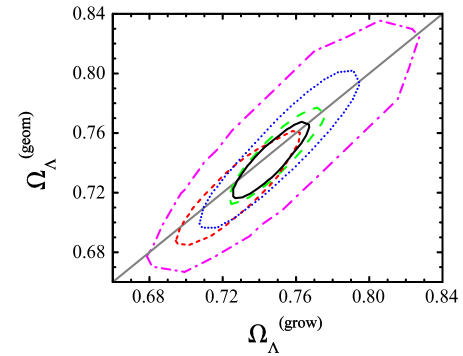
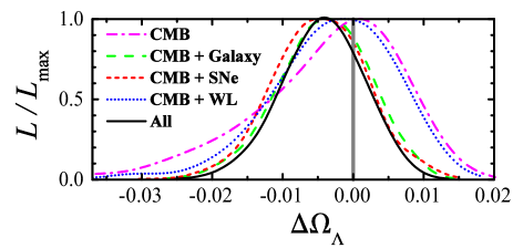
Applying our consistency test to the $\Lambda$CDM model, where the EOS parameters are fixed as $w^{\rm(geom)}=w^{\rm(grow)}=-1$, the upper panel in Fig. 1 shows the marginalized constraints on the $\Omega_{\Lambda}^{\rm(grow)}$ vs. $\Omega_{\Lambda}^{\rm(geom)}$ plane. The confidence contours follow roughly, but not exactly, the $\Omega_{\Lambda}^{\rm(geom)}=\Omega_{\Lambda}^{\rm(grow)}$ line. The interesting quantity in this case is the difference $\Delta\Omega_{\Lambda}\equiv\Omega_{\Lambda}^{\rm(geom)}-\Omega_{\Lambda}^{\rm(grow)}$, whose normalized probability distribution is shown in the lower panel of Fig. 1. When all data are utilized, we find the marginalized constraint $\Delta\Omega_{\Lambda}=-0.0044^{+0.0058+0.0108}_{-0.0057-0.0119}$ ($68\%$ and $95\%$ C.L. respectively). Figure 1 also shows that CMB anisotropies, when combined either with galaxy clustering or SNe, deliver most of the overall constraining power, i.e., having the narrowest likelihood distributions.

We also find the marginalized constraint on the average $\overline{\Omega}_{\Lambda}\equiv(\Omega_{\Lambda}^{\rm(geom)}+\Omega_{\Lambda}^{\rm(grow)})/2$ using all data sets: $\overline{\Omega}_{\Lambda}=0.744^{+0.016+0.030}_{-0.015-0.031}$. The constraint on the difference is almost three times better than the constraint on the average. The CMB contour in Fig. 1, even without the addition of other data, already exhibits this trend. Let us therefore focus on understanding this phenomenon in the context of CMB.

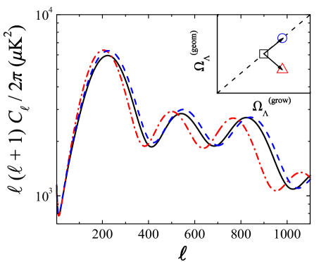
As illustrated in Fig. 2, increasing both $\Omega_{\Lambda}^{\rm(geom)}$ and $\Omega_{\Lambda}^{\rm(grow)}$ by the same amount (with all the other cosmological parameters fixed) produces only a small shift of the predicted $C_{\ell}$ (blue dashed curve). However, moving in the orthogonal direction, i.e., increasing $\Omega_{\Lambda}^{\rm(grow)}$ while decreasing $\Omega_{\Lambda}^{\rm(geom)}$, creates a much larger shift (red dot–dashed curve). It appears partial cancellations occur between the shift in the distance to last scattering (a geometrical quantity) and the shift in the sound horizon (which controls fluctuation growth) when one changes both $\Omega_{\Lambda}^{\rm(geom)}$ and $\Omega_{\Lambda}^{\rm(grow)}$ by the same small amount, creating a roughly degenerate direction along $\Omega_{\Lambda}^{\rm(geom)}=\Omega_{\Lambda}^{\rm(grow)}$. Conversely, the effects of the two different shifts roughly add when one changes $\Omega_{\Lambda}^{\rm(geom)}$ and $\Omega_{\Lambda}^{\rm(grow)}$ in opposite directions, making $\Delta\Omega_{\Lambda}$ highly constrained.

Figure 3: Joint constraints on $w^{\rm(geom)}$ and $w^{\rm(grow)}$ in a QCDM model (upper panel) and the normalized likelihood distribution of $\Delta w\equiv w^{\rm(geom)}-w^{\rm(grow)}$ (lower panel). Here the energy density parameters are fixed as $\Omega_{\rm DE}^{\rm(geom)}=\Omega_{\rm DE}^{\rm(grow)}$. The contours and curves show the $68\%$ confidence limits from the marginalized distributions. The thick gray lines show $w^{\rm(geom)}=w^{\rm(grow)}$. The data sets used are described in the text. Different contours and curves represent constraints from different combinations of the data sets (see legend in Fig. 1). The smallest contour and the most narrow curve (black solid line) represent constraints from all the data. No significant difference is found and deviations are constrained to $\Delta w=0.37^{+0.37+1.09}_{-0.36-0.53}$ ($68\%$ and $95\%$ C.L.). The star–shaped symbol corresponds to the effective $w^{\rm(geom)}$ and $w^{\rm(grow)}$, which approximately match the expansion history and the growth history, respectively, of a flat DGP model with our best–fit $\Omega_{m}$.

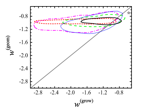
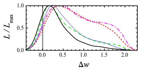
One could argue that in theories of modified gravity constructed to explain the late time cosmic acceleration, the growth of fluctuations should only deviate from GR at late times. A better approximation of such theories is perhaps to split the EOS parameter $w$. We therefore next apply our consistency test to the more general QCDM model. The EOS parameters, $w^{\rm(grow)}$ and $w^{\rm(geom)}$, are assumed constant, but are allowed to vary independently. In this test, we assume $\Omega_{\rm DE}^{\rm(geom)}=\Omega_{\rm DE}^{\rm(grow)}$. The upper panel in Fig. 3 shows the marginalized constraints in the $w^{\rm(grow)}$ vs. $w^{\rm(geom)}$ plane footnote5 . We again find that the difference $\Delta w\equiv w^{\rm(geom)}-w^{\rm(grow)}$ is consistent with zero; deviations are constrained by combining all data to $\Delta w=0.37^{+0.37+1.09}_{-0.36-0.53}$ (lower panel in Fig. 3). The average is constrained to be $\overline{w}\equiv(w^{\rm(geom)}+w^{\rm(grow)})/2=-1.13^{+0.18+0.28}_{-0.20-0.55}$.

Figure 3 shows a long tail towards large negative values of $w^{\rm(grow)}$, which can be understood as follows. Density perturbations can grow significantly only during the matter–dominated epoch, and as $w^{\rm(grow)}$ becomes more negative, this epoch is longer (i.e., dark energy domination occurs more recently). The extension of the likelihood contours in the large negative direction of $w^{\rm(grow)}$ reflects the fact that a very recent dark energy domination is actually acceptable as far as the growth of structure is concerned. This does not imply the data is consistent with the absence of dark energy, however. On the contrary, the data prefer a low $\Omega_{m}$ which for a flat universe implies the presence of $\Omega_{\rm DE}$. It is interesting to note that qualitatively, the DGP theory prefers $w^{\rm(grow)}>w^{\rm(geom)}$ LSS ; footnote1 , a region that is quite restricted by data already. In fact, we find that a DGP model with our best–fit $\Omega_{m}$, represented effectively by the star–shaped symbol in Fig. 3, lies beyond the $3\sigma$ contour for constraints from all the data sets; varying $\Omega_{m}$ in the DGP model within its $3\sigma$ limits has little effect on the position of the point. We also find the upper limits of $w^{\rm(grow)}<-0.97$ at $1\sigma$ and $w^{\rm(grow)}<-0.80$ at $2\sigma$ footnote6 .

VIII Discussions

Our study reveals no evidence of a discrepancy between the two split meta–parameters. The difference is consistent with zero at the 1$\sigma$ level for the $\Lambda$CDM model and 2$\sigma$ level for the QCDM model. We find tight constraints from the existing data sets, especially on the difference between $\Omega_{\Lambda}$ derived from growth and $\Omega_{\Lambda}$ derived from geometry (better than $1\%$). In other words, the cosmological constant model fits current data very well. Current data do not appear to demand modified gravity theories. Parameter splitting can be thought of as a crude way to parametrize the space of these theories. As such, our constraints can be viewed as putting restrictions on modified gravity theories, but the precise constraints on any particular theory must be worked out on a case by case basis. The kind of constraints we obtain here are likely to significantly improve in the future, as the cosmological data improve in quality and quantity. The power of future surveys is demonstrated by a calculation that a Large Synoptic Survey Telescope (LSST)–like survey could constrain $\Delta w$ to $0.04$, using shear tomography alone, an order of magnitude better than current constraint from all data sets ZHS ; JZ .