Measuring dark energy properties with 3D cosmic shear

Abstract

We present parameter estimation forecasts for present and future 3D cosmic shear surveys. We demonstrate in particular that, in conjunction with results from cosmic microwave background (CMB) experiments, the properties of dark energy can be estimated with very high precision with large-scale, fully 3D weak lensing surveys. In particular, a 5-band, 10,000 square degree ground-based survey of galaxies to a median redshift of $z_{m}=0.7$ could achieve $1$-$\sigma$ marginal statistical errors, in combination with the constraints expected from the CMB Planck Surveyor, of $\Delta w_{0}=0.108$ and $\Delta w_{a}=0.099$. We parameterize the redshift evolution of $w$ by $w(a)=w_{0}+w_{a}(1-a)$ where $a$ is the scale factor. Such a survey is achievable with a wide-field camera on a $4$ metre class telescope. The error on the value of $w$ at an intermediate pivot redshift of $z=0.368$ is constrained to $\Delta w(z=0.368)=0.0175$. We compare and combine the 3D weak lensing constraints with the cosmological and dark energy parameters measured from planned Baryon Acoustic Oscillation (BAO) and supernova Type Ia experiments, and find that 3D weak lensing significantly improves the marginalized errors on $w_{0}$ and $w_{a}$ in combination, and provides constraints on $w(z)$ at a unique redshift through the lensing effect. A combination of 3D weak lensing, CMB and BAO experiments could achieve $\Delta w_{0}=0.037$ and $\Delta w_{a}=0.099$. We also show how our results can be scaled to other telescopes and survey designs. Fully 3D weak shear analysis avoids the loss of information inherent in tomographic binning, and we also show that the sensitivity to systematic errors in photometric redshift is much less. In conjunction with the fact that the physics of lensing is very soundly based, the analysis here demonstrates that deep, wide-angle 3D weak lensing surveys are extremely promising for measuring dark energy properties.

1 Introduction

Our knowledge of cosmology has advanced considerably in recent years. Led by detailed measurements of the microwave background radiation and large-scale structure, many of the most important cosmological parameters are now known with good accuracy. This advance has come about principally through the all-sky maps of the microwave sky taken with the Wilkinson Microwave Anisotropy Probe (WMAP) (Bennett et al., 2003), supplemented by higher-resolution observations of the Arcminute Cosmology Bolometer Array Receiver (ACBAR) and Cosmic Background Imager (CBI) (Kuo et al., 2004; Pearson et al., 2003). When combined with large-scale structure information from the Anglo-Australian 2 degree field galaxy redshift survey (2dFGRS) (Colless et al., 2001; Percival et al., 2001), the Lyman-$\alpha$ forest (Croft et al., 2002; Gnedin and Hamilton, 2002), and measurements of galaxy bias (Verde et al., 2002), the data establish the concordance model of an accelerating Universe dominated by dark energy and dark matter (Spergel et al., 2003; Spergel et al., 2006). The acceleration of the Universe is also apparent in observations of distant supernovae (e.g. Riess et al., 2000). The determination of the density, baryon content and expansion rate of the Universe shifts the major unanswered questions in cosmology to the nature of the dark matter and dark energy. Dark energy in particular can be probed through its cosmological effects on the distance-redshift relation and the growth rate of structure.

The question of the precise nature of the dark energy is a far-reaching one. We use the simplest phenomenological model of dark energy by parameterizing the equation of state of the vacuum,

$$w\equiv p/(\rho c^{2}),$$ (1)

where $\rho$ is its energy-density and $p$ is the dark-energy/vacuum-pressure. $w=w(a)$ may vary with scale factor. If it is found with high precision that $w=-1$, then the dark energy cannot be distinguished with large-scale measurements from a modification to the gravity law along the lines suggested by Einstein with the cosmological constant. If, however, it can be established with a degree of certainty that $w$ differs from $-1$ at any redshift, then it cannot be associated with such a change to the gravity law, and is most naturally accounted for by a new field. This would be an extremely important discovery, and the time-evolution of the field would be a useful constraint on models. Some possibilities exist in the literature, such as those proposed by Ratra and Peebles (1988), but none is a clear favourite candidate.

Weak lensing is a very attractive proposition for studying dark energy, as it is sensitive to both of these effects, and, equally importantly, the physics of weak lensing is well understood. A key part of this is that it is sensitive to the distribution of matter in the Universe, regardless of its form. Furthermore, since weak lensing analysis can be done in a way which is either dependent on the distance-redshift relation alone (see e.g. Taylor et al., 2006; Jain & Taylor, 2003) or on both the distance-redshift relation and the growth factor (this paper), it can in principle distinguish between modified gravity models and dark energy models.

The main lesson of the field of microwave background astronomy is that with well-understood physics, robust results can be obtained with high precision. Weak lensing observations are, however, a technical challenge, as the imaging requirements are severe. Thus, it has only been in the last five years or so that the first measurements of cosmic shear have appeared (Bacon, Refregier and Ellis, 2000; Kaiser, Wilson and Luppino, 2000; van Waerbeke et al., 2000; Wittman et al., 2000). Weak lensing measurements to date have concentrated on obtaining the matter density parameter $\Omega_{m}$ and the amplitude of mass density fluctuations (Hoekstra, Yee and Gladders, 2002; Jarvis et al., 2003; Rhodes et al., 2004; Heymans et al., 2004; Hoekstra et al., 2006; Semboloni et al., 2006). More ambitiously, weak lensing observations have started to put constraints on the equation of state of dark energy (Jarvis et al., 2005; Semboloni at al., 2006). Theoretically, the prospects for determining dark energy properties (specifically its equation of state $w$) using weak lensing have been explored in a number of papers (e.g. Taylor et al., 2006; Hu and Tegmark, 1999; Huterer, 2002; Heavens, 2003; Refregier, 2003; Simon, King and Schneider, 2004; Takada and Jain, 2004; Song and Knox, 2004; Ishak et al., 2004; Ishak, 2005). The prospects for determining $w$ as a function of redshift $z$ are markedly improved when 3D information on the individual lensed sources is available. Source distances could come from spectroscopic redshifts, but given the depth and the sky area required, they are more likely to be estimated from photometric redshifts. With 3D information, the lensing pattern can be analyzed in shells at different distances (e.g. Hu, 1999; Hu and Jain, 2004; Ishak, 2005), or by analyzing the shear pattern as a fully three-dimensional field (Heavens, 2003). It is the latter possibility which we investigate in this paper. The statistical properties of the shear pattern are influenced by many cosmological parameters, including $w(z)$. In this paper we extend the analysis of Heavens (2003) to small-angle surveys as well as computing the expected marginal errors on $w$ (and its evolution), using a Fisher matrix approach. We investigate issues of depth vs area, and the number of photometric bands which should be used, to determine the dark energy properties as accurately as possible. The main focus of the paper is in computing the expected statistical errors, but we do consider the impact of some systematics (Ishak et al., 2004; Bernstein, 2005; Huterer et al., 2005).

The layout of the paper is as follows: in Section 2 we detail the transform method used and compute the covariance matrix of the transform coefficients; in Section 3 we outline how the expected statistical errors on parameters are calculated; in Section 4 we present the survey design and how we can scale to other surveys and in Section 5 we present an optimization of survey design and the parameter errors; in Section 6 we consider the synergy of 3D weak lensing with other dark energy probes and discuss future surveys and finally we give our conclusions in Section 7.

2 Method

2.1 Transformation of scalar and shear fields

The observable quantities we use are the estimates of the shear field at locations in three dimensions. The estimates of the complex shear come from the shape and orientation of galaxies, where the radial distance is obtained approximately by using photometric redshift estimates obtained from observations through several or many filters.

In a previous paper (Heavens, 2003) we introduced the idea of 3D weak lensing analysis in harmonic space as a statistical tool. In Castro, Heavens and Kitching (2005), we developed the subject formally and found the power spectrum of 3D weak lensing shear. In this paper we consider the flat-sky limit including the non-linear evolution of the power spectrum. We consider a transform of the 3D shear field in spin-weight spherical harmonics and spherical Bessel functions. This is a very natural expansion for the shear field, as the complex shear $\gamma$ is a spin-weight 2 object, as are the spin-weight 2 spherical harmonics: under a local rotation of the coordinate system by angle $\psi$, $\gamma$ changes to $\gamma e^{2i\psi}$. The spherical harmonic transform of a spin-weight $s$ field ${}_{s}f({\bf r})$ is defined here by

$${}_{s}f_{\ell m}(k)\equiv\sqrt{2\over\pi}\,\int\,d^{3}{\bf r}_{s}f({\bf r})\,kj_{\ell}(kr)\,_{s}Y_{\ell}^{m*}({\hat{\bf n}})$$ (2)

where $j_{\ell}(z)$ is a spherical Bessel function, ${}_{s}Y_{\ell}^{m}$ a spin-weight $s$ spherical harmonic, $k$ is a radial wavenumber, $\ell$ is a positive integer, $m=-\ell,\ldots\ell$ and ${\hat{\bf n}}$ represents the direction $\theta$, $\varphi$. For $s=0$ the spin-weight spherical harmonics are the usual spherical harmonics $Y_{\ell}^{m}$, and this is the appropriate spherical expansion of a scalar field. Note the presence here of a benign factor of $k$, to agree with the notation of Castro, Heavens and Kitching (2005). The motivation for using spherical coordinates is manyfold: firstly the selection function for a survey can often be separated into an angular (sky coverage) part and a radial component; secondly the errors in photometric redshifts introduce purely radial errors in the positions of the source galaxies; thirdly, in the Born approximation, the lensing effect is an integral effect along the (radial) line of sight. The motivation in flat space for using products of spherical Bessel functions and spherical harmonics is that, as eigenfunctions of the Laplacian operator, it is easy to relate the expansion coefficients of the gravitational potential to those of the density field. Similar considerations led Heavens and Taylor (1995)(see also Fisher et al., 1994; Tadros et al., 1999; Percival et al., 2004) to expand the large-scale structure of galaxies in spherical Bessel functions and spherical harmonics. Since cosmic shear depends on the gravitational potential, the use of this basis allows us to relate the expansion of the shear field to the expansion of the mass density field. The properties of the latter depend in a calculable way on cosmological parameters, so this opens up the possibility of using 3D weak shear to estimate these quantities.

For surveys with large opening angles on the sky, a full expansion in spherical Bessel functions and spherical harmonics is the natural choice. Such an expansion is generally applicable, but for small-angle surveys whose signal is dominated by high-$\ell$ modes, the spherical harmonics are cumbersome and their accurate computation can present problems. For such surveys, we can approximate the spherical harmonics as sums of exponentials, as detailed in Appendix A of Santos et al. (2003).

For this paper we use the flat-sky expansion, which for a scalar ($s=0$) field reads

$$f(k,{{\mbox{\boldmath{$\ell$}}}})\equiv\sqrt{2\over\pi}\,\int\,d^{3}{\bf r}f({\bf r})kj_{\ell}(kr)\exp(-i{\mbox{\boldmath{$\ell$}}}\cdot\mn@boldsymbol{\theta}),$$ (3)

where $\ell$ is a 2D angular wavenumber and $k$ a radial wavenumber. In the spherical Bessel function, $\ell=|{\mbox{\boldmath{$\ell$}}}|$; $\ell$ is necessarily an integer, but we assume that $\ell\gg 1$ so that enforcing integer $\ell$ is a minor approximation. Note that we are performing a full 3D expansion of the shear field and assume a flat Universe except where indicated. An alternative approach to include at least some 3D information is what is referred to as tomography, where the shear pattern of galaxies is analyzed in shells, based on their photometric redshifts (Hu, 1999; Hu, 2002; Jain and Taylor, 2003; Takada and White, 2004). It is however evident that the binning process loses at least some information, and it is not necessary.

The inverse transform in the flat-sky approximation is

$$f({\bf r})=\sqrt{{2\over\pi}}\int{d^{2}{\mbox{\boldmath{$\ell$}}}\over(2\pi)^{2}}dk\,kj_{\ell}(kr)\exp(i{\mbox{\boldmath{$\ell$}}}.\mn@boldsymbol{\theta})f(k,{\mbox{\boldmath{$\ell$}}}).$$ (4)

The coefficients of the expansion in the two systems are related by generalization of equation (A13) in Santos et al. (2003):

$$f(k,{\mbox{\boldmath{$\ell$}}})=\sqrt{{2\pi\over\ell}}\sum_{m}i^{-m}f_{\ell m}(k)\exp(im\phi_{{\mbox{\tiny\boldmath{$\ell$}}}})$$ (5)

where the small survey is centred at the pole of the coordinate system, and the 2D transverse wavevector is ${\mbox{\boldmath{$\ell$}}}=(\ell\cos\phi_{{\mbox{\tiny\boldmath{$\ell$}}}},\ell\sin\phi_{{\mbox{\tiny\boldmath{$\ell$}}}})$. The covariances of the flat-sky coefficients are related to the power spectrum of $f$ by

$$\langle f(k,{\mbox{\boldmath{$\ell$}}})f^{*}(k^{\prime},{\mbox{\boldmath{$\ell$}}}^{\prime})\rangle=(2\pi)^{2}\,P_{f}(k)\,\delta^{D}(k-k^{\prime})\delta^{D}({\mbox{\boldmath{$\ell$}}}-{\mbox{\boldmath{$\ell$}}}^{\prime})$$ (6)

where $\delta^{D}$ is the Dirac delta function.

Our plan is essentially to transform the components of the 3D shear field to produce a set of transform coefficients as a function of $(k,{\bf{\mbox{\boldmath{$\ell$}}}}$). These data will depend on cosmological parameters, and can be used in a likelihood analysis to constrain those parameters.

2.1.1 Transformation of shear fields

The weak lensing shear components we transform are $\gamma_{1}({\bf r})$ and $\gamma_{2}({\bf r})$, which are related to the lensing potential $\phi({\bf r})$ through (e.g. Bartelmann and Schneider, 2001)

$$\gamma_{1}={1\over 2}\left(\phi_{11}-\phi_{22}\right);\qquad\gamma_{2}=\phi_{12}$$ (7)

where $\phi_{ij}\equiv\partial^{2}\phi/\partial\theta_{i}\partial\theta_{j}$. $\phi$ itself is dependent on cosmological parameters through its relation to the mass density field (see section 2.4). We will return to this dependence later. For a large-area survey, it is a measure of the shears with respect to axes based on the spherical coordinate system, in which case the complex shear $\gamma\equiv\gamma_{1}+i\gamma_{2}$ is the second edth derivative of $\phi$:

$$\gamma({\bf r})={1\over 2}\,\eth\,\,\eth\,\phi({\bf r}).$$ (8)

(Castro, Heavens and Kitching, 2005). In the flat-sky limit, $\,\eth\,\rightarrow-(\partial_{x}+i\partial_{y})$, where the $\partial_{x,y}\equiv\partial/\partial\theta_{x,y}$. Expanding the lensing potential in terms of spherical Bessel functions and exponential functions, as in equation (3), we see that it is natural to expand the complex shear field in terms of $\,\eth\,\,\eth\,\exp(-i{\mbox{\boldmath{$\ell$}}}.\mn@boldsymbol{\theta})=\ell^{2}X_{\mbox{\boldmath{$\ell$}}}\exp(-i{\mbox{\boldmath{$\ell$}}}.\mn@boldsymbol{\theta})$, where

$$X_{\mbox{\boldmath{$\ell$}}}\equiv{({\mbox{\boldmath{$\ell$}}}_{y}^{2}-{\mbox{\boldmath{$\ell$}}}_{x}^{2})+2i{\mbox{\boldmath{$\ell$}}}_{x}{\mbox{\boldmath{$\ell$}}}_{y}\over{\mbox{\boldmath{$\ell$}}}^{2}}.$$ (9)

The ${\mbox{\boldmath{$\ell$}}}^{2}$ in the denominator is included for convenience, so the inverse transform kernel is just $\sqrt{2/\pi}k\,j_{\ell}(kr)X_{\mbox{\boldmath{$\ell$}}}^{*}\exp(i{\mbox{\boldmath{$\ell$}}}.\mn@boldsymbol{\theta}_{g})$.

2.1.2 Fiducial Cosmology

An immediate issue to address is which radial coordinate to use in the spherical Bessel function. The observed quantities are the estimated redshifts of the sources, and we need to do two things: one is to translate these into radial distances; the second is to account for the error in the estimation of the redshifts. For the former, we choose a fiducial set of cosmological parameters, to define a transformation $r^{0}(z_{p})$ from the photometric redshift estimate $z_{p}$ to a radial coordinate $r^{0}$. For this paper, we choose as the fiducial model the concordance model (Spergel et al., 2006) with $\Omega_{m}=0.27$, $\Omega_{b}=0.04$, $\Omega_{v}=0.73$, $\sigma_{8}=0.8$, $h=0.71$, $w_{0}=-1$ and $w_{a}=0$ where the variables are the matter, baryon, vacuum density parameters, Hubble constant in units of $100\,$ km s${}^{-1}\,$Mpc^-1 and the dark energy equation of state parameters respectively. The equation of state of dark energy is modelled in terms of scale factor $a$ by

$$w(a)=w+w_{a}(1-a)$$ (10)

(Chevallier and Polarski, 2001; Linder, 2003) where $a(z)=(1+z)^{-1}$ is the cosmic scale factor normalized to unity at the present epoch.

We also include the scalar spectral index $n_{s}=1$ and its running $\alpha_{n}=0$. For the CMB Fisher calculations, see Section 5.1, we also include the tensor to scalar ratio $r=0.01$ and the optical depth to the surface of last scattering $\tau=0.09$.

2.2 Transformation

The lensing potential is defined everywhere, but we sample it only at the locations of galaxies, so it is natural to make a transformation of this point process, summing over galaxies rather than integrating over space. Our estimate of the transform is thus defined as

$$\hat{\gamma}(k,{\mbox{\boldmath{$\ell$}}})=\sqrt{{2\over\pi}}\sum_{g}\,\gamma({\bf r})kj_{\ell}(kr_{g}^{0})\exp(-i{\mbox{\boldmath{$\ell$}}}.\mn@boldsymbol{\theta}_{g})W(r_{g}^{0})$$ (11)

where $W(r)$ is an arbitrary weight function, and $(r_{g}^{0},\mn@boldsymbol{\theta}_{g})$ are the coordinates of galaxy $g$.

Note the appearance of two distances in the transform, $r$ and $r^{0}$ (at each galaxy $g$): the main application of this study is to determine cosmological parameters, which affects the $r(z)$ relation. The shear field is the shear field at the actual coordinate ${\bf r}_{g}$ of the galaxy, and this depends on the true cosmological parameters, whereas the expansion (and weighting) is done with the fiducial model parameters. This distinction was neglected in Heavens (2003) and leads to an underestimate of the errors on the dark energy equation of state in that paper; the error estimates for the power spectrum in that paper are unaffected by this error.

Writing the number density of source galaxies $n({\bf r})$ as the sum of a set of delta functions, we see that

$$\hat{\gamma}(k,{\mbox{\boldmath{$\ell$}}})=\sqrt{{2\over\pi}}\int d^{3}{\bf r}\,n({\bf r})\gamma({\bf r})\,k\,j_{\ell}(kr^{0})\exp(-i{\mbox{\boldmath{$\ell$}}}\cdot\mn@boldsymbol{\theta})W^{0},$$ (12)

where $W^{0}=W(r^{0})$. Note that in the high-$\ell$ limit these are also the (minus) coefficients of the expansion of the convergence field $\kappa$ (Castro, Heavens and Kitching, 2005). This has an expectation value which is obtained by replacing $n({\bf r})$ by the mean density of the source galaxies, $\bar{n}(r)$. Here we assume that selection effects are uniform across the survey so there is no angular dependence. Thus the $\hat{\gamma}$ are estimators of

$$\gamma(k,{\mbox{\boldmath{$\ell$}}})\equiv\sqrt{{2\over\pi}}\int d^{3}{\bf r}\,\bar{n}(r)\gamma({\bf r})\,kj_{\ell}(kr^{0})\exp(-i{\mbox{\boldmath{$\ell$}}}.\mn@boldsymbol{\theta})W^{0}.$$ (13)

The estimates will differ because of the discrete nature of the galaxies, which leads to shot noise, the photometric redshift errors, and the source clustering. For deep surveys, and with a radial smoothing arising from the photometric redshifts, source clustering can be safely ignored. We include the effects of photometric errors, but ignore uncertainties in the photometric redshift distribution. In terms of the observable photometric redshift distribution of sources (all-sky), $\bar{n}(r)d^{3}{\bf r}=\bar{n}_{z}(z_{p})dz_{p}/4\pi$, we have

$$\gamma(k,{\mbox{\boldmath{$\ell$}}}) \equiv \sqrt{{1\over 8\pi^{3}}}\int dz_{p}\,d^{2}\mn@boldsymbol{\theta}\,\bar{n}_{z}(z_{p})\gamma({\bf r})\,kj_{\ell}(kr^{0})$$

$$\exp(-i{\mbox{\boldmath{$\ell$}}}\cdot\mn@boldsymbol{\theta})W^{0}.$$

2.3 Photometric redshift errors

Photometric redshifts lead to a smoothing of the distribution in the radial direction. If we denote by $p(z_{p}|z)$ the probability of the photometric redshift being $z_{p}$, given that the true redshift is $z$, the mean of the expansion coefficients will be

$$\gamma(k,{\mbox{\boldmath{$\ell$}}}) \equiv \sqrt{{1\over 8\pi^{3}}}\int dz\,dz_{p}d^{2}\mn@boldsymbol{\theta}\,p(z_{p}|z)\,\bar{n}_{z}(z_{p})$$

$$\gamma({\bf r})\,kj_{\ell}(kr^{0})\exp(-i{\mbox{\boldmath{$\ell$}}}\cdot\mn@boldsymbol{\theta})W^{0}.$$

Note that $p(z_{p}|z)$ is arbitrary; it will generally have a dispersion which depends on redshift, and can, if desired, include broad wings to account for a small percentage of catastrophic failures in the photometric redshift estimates. We assume a Gaussian, with a $z$-dependent dispersion:

$$p(z_{p}|z)={1\over\sqrt{2\pi}\sigma_{z}(z)}\exp\left[-(z_{p}-z+z_{\rm bias})^{2}\over 2\sigma_{z}^{2}(z)\right].$$ (16)

$z_{\rm bias}$ is a possible bias in the photometric redshift calibration, the effect of this on dark energy parameters is discussed in Section 5.5.1. Strictly the shear is estimated at the actual radial coordinate of the galaxy, which may differ from $r(z)$ because of peculiar velocities. We can safely ignore these, whose effect is small compared with current photometric redshift errors.

2.4 Relationship of $\gamma(k,{\mbox{\boldmath{$\ell$}}})$ to cosmological parameters

The lensing potential $\phi$ is related to the peculiar gravitational potential $\Phi$ by a radial line-of-sight integral (e.g. Bartelmann and Schneider, 2001):

$$\phi({\bf r})={2\over c^{2}}\int_{0}^{r}dr^{\prime}F_{K}(r,r^{\prime})\Phi({\bf r}^{\prime}).$$ (17)

where $F_{K}(r,r^{\prime})\equiv\left\{f_{K}(r-r^{\prime})/\left[f_{K}(r)f_{K}(r^{\prime})\right]\right\}$, and $f_{K}(r)d\psi$ is the dimensionless transverse comoving separation for points separated by an angle $d\psi$. The Robertson-Walker metric may be written $ds^{2}=c^{2}dt^{2}-R^{2}(t)\left[dr^{2}+f_{K}^{2}(r)d\psi^{2}\right]$, and $f_{K}(r)$ takes the values $\sin r,\ r,\ \sinh r$ for curvature values $k=1,0,-1$. For a flat Universe $F_{K}(r,r^{\prime})=(1/r^{\prime}-1/r)$.

The peculiar gravitational potential is related to the overdensity field $\delta({\bf r})\equiv\left[\rho({\bf r})-\bar{\rho}\right]/\bar{\rho}$ by the comoving Poisson’s equation

$$\nabla^{2}\Phi={3\Omega_{m}H_{0}^{2}\over 2a(t)}\delta,$$ (18)

where $\Omega_{m}$ is the present-day matter density parameter, $H_{0}$ is the present Hubble constant and $a(t)=R(t)/R_{0}=1/(1+z)$ is the scale factor.

Note that $\delta$ itself is not a homogeneous field, because it evolves with time, and hence with distance from the observer through the light travel time. We get around the subtleties of this by defining at each epoch a homogeneous field by referring all field measurements to that time. Thus we can, for example, define a power spectrum which is time-dependent, and hence $r$-dependent. This may seem a little strange, since we have transformed from ${\bf r}$ space. The transforms of the homogeneous fields will be denoted by $\delta(k,{\mbox{\boldmath{$\ell$}}};r)$ etc.

For high $\ell$, the transforms of $\Phi$ and $\delta$ (referred to epoch $t$ or equivalently $r$) are related simply by

$$\Phi(k,{\mbox{\boldmath{$\ell$}}};r)=-{3\Omega_{m}H_{0}^{2}\over 2k^{2}a(t)}\delta(k,{\mbox{\boldmath{$\ell$}}};r).$$ (19)

Inserting these definitions in the equation for $\gamma(k,{\mbox{\boldmath{$\ell$}}})$,we find the relationship between $\gamma(k,{\mbox{\boldmath{$\ell$}}})$ and the transform of $\delta$:

$$\gamma(k,{\mbox{\boldmath{$\ell$}}}) = -{3\Omega_{m}H_{0}^{2}\over 2\pi^{2}c^{2}}\int_{0}^{\infty}dzdz_{p}p(z_{p}|z)$$

$$\!\!\!\!\!\!\!\!\!\!\!\int{d^{2}\mn@boldsymbol{\theta}}\,kj_{\ell}(kr^{0})W^{0}\,\bar{n}_{z}(z_{p})\exp(-i{\mbox{\boldmath{$\ell$}}}.\mn@boldsymbol{\theta})$$

$$\!\!\!\!\!\!\!\!\!\!\!\int_{0}^{r}dr^{\prime}a^{-1}(r^{\prime})\,F_{K}(r,r^{\prime})$$

$$\!\!\!\!\!\!\!\!\!\!\!\int dk^{\prime}{d^{2}{\mbox{\boldmath{$\ell$}}}^{\prime}\over(2\pi)^{2}}\,k^{\prime}j_{\ell^{\prime}}(k^{\prime}r^{\prime})\delta(k^{\prime},{\mbox{\boldmath{$\ell$}}}^{\prime};r^{\prime})\frac{X_{{\mbox{\boldmath{$\ell$}}}^{\prime}}}{2}\exp(i{\mbox{\boldmath{$\ell$}}}^{\prime}.\mn@boldsymbol{\theta}).$$

Integration over $\mn@boldsymbol{\theta}$ gives $(2\pi)^{2}\delta^{D}({\mbox{\boldmath{$\ell$}}}-{\mbox{\boldmath{$\ell$}}}^{\prime})$, so

$$\gamma(k,{\mbox{\boldmath{$\ell$}}}) = -{3X_{\mbox{\boldmath{$\ell$}}}\Omega_{m}H_{0}^{2}\over 4\pi^{2}c^{2}}\int_{0}^{\infty}dzdz_{p}p(z_{p}|z)\bar{n}_{z}(z_{p})\,$$

$$\!\!\!\!\!\!\!\!\!\!\!\!\!\!\!\!\!\!\!\!\!\!\!j_{\ell}(kr^{0})W^{0}\int_{0}^{r}dr^{\prime}F_{K}(r,r^{\prime})(1+z^{\prime})$$

$$\!\!\!\!\!\!\!\!\!\!\!\!\!\!\!\!\!\!\!\!\!\!\!\int dk^{\prime}\,k^{\prime}j_{\ell}(k^{\prime}r^{\prime})\,\delta(k^{\prime},{\mbox{\boldmath{$\ell$}}};r^{\prime}).$$

This is a fundamental result of this paper. It establishes the connection between the (observable) 3D shear transform coefficients, and the underlying matter density fluctuations, whose properties are calculable from theory.

2.5 Covariance matrix of $\gamma(k,{\mbox{\boldmath{$\ell$}}})$

The signal part of the covariance matrix of the $\gamma(k,{\mbox{\boldmath{$\ell$}}})$ is obtained from equation (2.4). For the covariance of the overdensity field coefficients, it is algebraically convenient to use the geometric mean of the power spectra $P_{\delta}$, rather than the power spectrum evaluated at epochs corresponding to $r$ or $r^{\prime}$. Both of these could also be justified; note also that $P_{\delta}$ does not depend on $\ell$ (Castro, Heavens and Kitching, 2005).

$$\langle\delta(k,{\mbox{\boldmath{$\ell$}}};r)\delta^{*}(k^{\prime},{\mbox{\boldmath{$\ell$}}}^{\prime};r^{\prime})\rangle \simeq (2\pi)^{2}\sqrt{P_{\delta}(k;r)P_{\delta}(k^{\prime};r^{\prime})}$$

$$\delta^{D}(k-k^{\prime})\delta^{D}({\mbox{\boldmath{$\ell$}}}-{\mbox{\boldmath{$\ell$}}}^{\prime}).$$

The covariance matrix for the shear expansion coefficients is then

$$\langle\gamma(k,{\mbox{\boldmath{$\ell$}}})\gamma^{*}(k^{\prime},{\mbox{\boldmath{$\ell$}}}^{\prime})\rangle_{S}=Q_{\ell}\,(k,k^{\prime})\,\delta^{D}({\mbox{\boldmath{$\ell$}}}-{\mbox{\boldmath{$\ell$}}}^{\prime})$$ (23)

where $Q_{\ell}\,(k,k^{\prime})$ can be written as

$$Q_{\ell}(k,k^{\prime})={9\Omega_{m}^{2}H_{0}^{4}X_{{\mbox{\boldmath{$\ell$}}}}^{2}\over 4\pi^{2}c^{4}}\int{d\tilde{k}\over\tilde{k}^{2}}\,G_{\ell}(k,\tilde{k})G_{\ell}(k^{\prime},\tilde{k})$$ (24)

where

$$G_{\ell}(k,\tilde{k})\equiv\int dz\,dz_{p}\,\bar{n}_{z}(z_{p})W(z_{p})p(z_{p}|z)U_{\ell}(r,\tilde{k})j_{\ell}(kr^{0})$$ (25)

and

$$U_{\ell}(r,k)\equiv\int_{0}^{r}d\tilde{r}\,{F_{K}(r,\tilde{r})\over a(\tilde{r})}\sqrt{P_{\delta}(k;\tilde{r})}\,j_{\ell}(k\tilde{r}).$$ (26)

where $r=r(z)$ etc. Equation (23) is the second important result of the paper.

2.6 Shot noise

The shot noise can be calculated by making the usual assumption that the galaxies are a Poisson sampling of an underlying smooth field (see e.g. Peebles, 1980). In practice we consider estimators of the transforms of the individual components of the shear, $\gamma_{\alpha};\ \alpha=1,2$. In the normal way for a point process, these may be written as sums over small cells $c$, each of which contains $n_{c}=0$ or 1 galaxy:

$$\hat{\gamma}_{\alpha}(k,{\mbox{\boldmath{$\ell$}}})\equiv\sqrt{{2\over\pi}}\sum_{\rm cells\ c}n_{c}\gamma_{\alpha c}({\bf r}_{c})\,kj_{\ell}(kr^{0}_{c})\exp(-i{\mbox{\boldmath{$\ell$}}}\cdot\mn@boldsymbol{\theta}_{c})W^{0}.$$ (27)

The variance of this involves a double sum over cells, and the averaging over cells $c$ and $d$, $\langle n_{c}n_{d}\rangle$ contains shot noise terms when $c=d$, in which case $\langle n_{c}^{2}\rangle=\langle n_{c}\rangle$, and the shot noise reduces to a single sum, or an integral when we move back to a continuum description. Using the fact that the variance of the shear estimate for a single galaxy is completely dominated by the variance in the intrinsic ellipticity of the galaxy, $\sigma_{e}^{2}$, rather than by lensing,

$$\langle\gamma_{\alpha}\gamma_{\beta}^{*}\rangle={\sigma_{e}^{2}\over 2}\delta^{K}_{\alpha\beta}$$ (28)

where $\delta^{K}$ is a Kronecker delta function, and $\sigma_{e}\simeq 0.3$ (Brown et al., 2003), we find an expression for the shot noise as

$$\langle\hat{\gamma}_{\alpha}(k,{\mbox{\boldmath{$\ell$}}})\hat{\gamma}_{\beta}^{*}(k^{\prime},{\mbox{\boldmath{$\ell$}}}^{\prime})\rangle_{SN} = \sigma_{e}^{2}\int dz\,\bar{n}_{z}(z)kj_{\ell}(kr^{0})$$

$$k^{\prime}j_{\ell}(k^{\prime}r^{0})W^{2}(z)\,\delta^{K}_{\alpha\beta}\,\delta^{D}({\mbox{\boldmath{$\ell$}}}-{\mbox{\boldmath{$\ell$}}}^{\prime}).$$

3 Estimation of cosmological parameters

Cosmological parameters influence the shear transforms in a number of ways: the matter power spectrum $P_{\delta}(k;t)$ is dependent on $\Omega_{m}$, $h$ and the linear amplitude $\sigma_{8}$. The linear power spectrum is dependent on the growth rate, which also has some sensitivity to the vacuum energy equation of state parameter $w(z)$. $w$ also affects the $r(z)$ relation and hence the angular diameter distance $f_{K}[r(z)]$. These parameters ($\{\Theta_{\alpha}\}$) may be estimated from the data using likelihood methods. Assuming uniform priors for the parameters, the maximum a posteriori probability for the parameters is given by the maximum likelihood solution. We use a Gaussian likelihood

$$2\ln L({\bf g}|\{\theta_{\alpha}\})={\rm constant}-\det(C)-{\bf g}\cdot C^{-1}\cdot{\bf g}$$ (30)

where $C=S+N$ is the covariance matrix, given by signal and noise terms equations (23) and (2.6). Note that the average values of $\gamma(k,{\mbox{\boldmath{$\ell$}}})$ is zero, so the information on the parameters comes from the dependence of the signal part of the covariance matrix $C$. i.e. we adjust the parameters until the covariance of the model matches that of the data. This was the approach of Heavens and Taylor (1995); Ballinger, Heavens and Taylor (1995); Tadros et al. (1999); Percival et al. (2004) in analysis of large-scale galaxy data. For many surveys, many useful modes of the shear transform have contributions from wavenumbers where the power spectrum is quite nonlinear. The use of a Gaussian likelihood thus needs to be justified by comparison with simulated data; this will be explored in a later paper, and it is possible that a different likelihood function may be necessary in the non-linear régime.

3.1 Expected errors on cosmological parameters - the Fisher matrix

The expected errors on the parameters can be estimated with the Fisher information matrix (Jungman et al., 1996; Tegmark, Taylor and Heavens, 1997). This has the great advantage that different observational strategies can be analyzed and this can be very valuable for experimental design. The Fisher matrix gives the best errors to expect, and should be accurate if the likelihood surface near the peak is adequately approximated by a multivariate Gaussian.

The Fisher matrix is the expectation value of the second derivative of the $\ln L$ with respect to the parameters $\Theta_{\alpha}$:

$$F_{\alpha\beta}=-\left\langle{\partial^{2}\ln L\over\partial\Theta_{\alpha}\partial\Theta_{\beta}}\right\rangle$$ (31)

and the marginal error on parameter $\Theta_{\alpha}$ is $\sqrt{(F^{-1})_{\alpha\alpha}}$. If the means of the data are fixed, the Fisher matrix can be calculated from the covariance matrix and its derivatives (Tegmark, Taylor and Heavens, 1997) by

$$F_{\alpha\beta}={1\over 2}{\rm Trace}\left[C^{-1}C_{,\alpha}C^{-1}C_{,\beta}\right].$$ (32)

For a square patch of sky, the Fourier transform leads to uncorrelated modes, provided the modes are separated by $2\pi/L$ where $L$ is the side of the square in radians, and the Fisher matrix is simply the sum of the Fisher matrices of each $\ell$ mode:

$$F_{\alpha\beta}={1\over 2}\sum_{\mbox{\tiny\boldmath{$\ell$}}}{\rm Trace}\left[(C^{\mbox{\tiny\boldmath{$\ell$}}})^{-1}C^{\mbox{\tiny\boldmath{$\ell$}}}_{,\alpha}(C^{\mbox{\tiny\boldmath{$\ell$}}})^{-1}C^{\mbox{\tiny\boldmath{$\ell$}}}_{,\beta}\right],$$ (33)

where $C^{\mbox{\tiny\boldmath{$\ell$}}}$ is the covariance matrix for a given $\ell$ mode. We compute $C^{\mbox{\tiny\boldmath{$\ell$}}}$ numerically from the signal and noise parts equations (23) and (2.6), for given $\bar{n}_{z}(z)$, photometric redshift error distribution, cosmology and survey area, which governs the separation of uncorrelated $\ell$ modes.

4 Survey Design Formalism

In this Section we discuss the survey design factors. We start by detailing the assumptions of the survey design, and discuss some details of the Fisher matrix calculation. Possible future weak lensing surveys and their effectiveness are discussed in the Section 5.

4.1 Survey parameters

In assigning survey parameters we follow the formalism detailed in Taylor et al. (2006). We assume that the redshift distribution for a typical magnitude-limited survey is of the form

$$\bar{n}(z)\propto z^{2}\exp\left[-\left({z\over z_{0}}\right)^{1.5}\right]$$ (34)

where $z_{0}=z_{m}/1.412$, and $z_{m}$ is the median redshift of the survey (e.g. Baugh and Efstathiou, 1993).

Figure 1: The photometric errors as a function of redshift $z$ for a 5-band (upper solid) and a 17-band (lower solid) optical survey. The dashed line has $\sigma_{z}(z)=0.05(1+z)$ for comparison.

The number density of useable sources with photometric redshift and shape estimates is taken to scale as

$$n_{0}=30z_{m}^{3.4}\ \ {\rm per\ square\ arcminute}.$$ (35)

This was estimated from the COMBO-17 survey. We take a maximum redshift of $z_{\rm max}=1.5$ for ground based surveys. This is due to the difficulty of measuring galaxy shape, because of the decrease in a galaxy’s apparent size with increasing redshift, coupled with the seeing limit.

We assume that the photometric redshift errors are Gaussian, with a dispersion given by $\sigma(z)=\sigma_{0}(1+z)f(m,z)$, where $m$ is the apparent magnitude of the galaxy, the function $f(m,z)$ is given in Taylor et al. (2006). We integrate over a Schechter function to get the average error as a function of $z$. The error distribution is shown for a 5-band optical survey and a 17-band optical survey in Figure 1. The assumption of Gaussianity of $p(z_{p}|z)$ can easily be relaxed: outliers can, for example, be included, we investigate this in Section 5.5.2. We have extrapolated these formula to $z=1.5$, though this extrapolation may be optimistic as photometric redshift estimates can increases dramatically at $z\approx 1$ if IR data is not available.

The variables which can be varied are the area $A$ and depth of the survey ($z_{m}$), and the number of bands. These scale with the number of nights observing $T$, the telescope diameter $D$ and the field-of-view $F$ as (see Taylor et al., 2006)

$$T\propto z_{m}^{4}AD^{-2}F^{-1}.$$ (36)

We consider as our default survey a $4$ metre telescope with a $2$ square degree field-of-view which could observe an area of $10$,$000$ square degrees to $z_{m}=0.7$ with $5$-bands in $600$ nights of observing, this could be achievable with surveys such as darkCAM (Taylor, 2005; conference proceedings of Probing the Dark Universe with Subaru and Gemini) or the Dark Energy Survey (Wester, 2005).

We compute the nonlinear power spectrum using the fitting formulae of Smith et al. (2003), based on linear growth rates given by Linder and Jenkins (2003). In order to avoid the high-$k$ régime where the formulae may be unreliable, or where baryonic effects might alter the power spectrum ($k>10hMpc^{-1}$; White, 2004; Zhan & Knox, 2004), we do not analyse modes with $k>1.5\,Mpc^{-1}$. Note that the non-local nature of lensing does mix modes to some degree, but these modes are sufficiently far from the uncertain highly-nonlinear régime that this is not a concern (Castro, Heavens and Kitching, 2005). In any case the results are very insensitive to the radial $k$ limit, since the photometric redshift errors supress radial power at much lower $k$. We include angular modes as small as each survey will allow, and analyse up to $\ell_{\rm max}=5000$. We note that the intracluster medium might affect the power spectrum on the level of a few percent for $1000\mathrel{\raise 1.16pt\hbox{$<$}\kern-7.0pt\lower 3.06pt\hbox{{$\scriptstyle\sim$}}}\ell\mathrel{\raise 1.16pt\hbox{$<$}\kern-7.0pt\lower 3.06pt\hbox{{$\scriptstyle\sim$}}}3000$ (Zhan & Knox, 2004). These modes will still contain useful information, but a more detailed analysis might be nessacary when the method is applied. To help asses the extent of any modification to the expected accuracy, we also quote results for a more conservative limit of $\ell_{\rm max}=2000$, this increases the predicted marginalised errors by approximately $0.01$. The flat-sky approximation will break down for the low-$\ell$ modes, but there is little power there in any case (Figure 2).

Figure 2: The contributions to the Fisher matrix element $F_{ww}$ from different ranges of $\ell$ for a 10,000 square degree survey with $z_{m}=0.70$ and 5 bands. $w=w_{0}$ in this Figure for clarity.

We allow for a Universe with the following parameters: $\Omega_{m}$, $\Omega_{v}$, $h$, $\sigma_{8}$, $\Omega_{b}$, $w_{0}$, $w_{a}$, $n_{s}$ and $\alpha_{n}$. $\sigma_{8}$ represents the amplitude of the perturbations, $n_{s}$ the scalar spectral index and its running $\alpha_{n}$, and we parameterize $w(a)$ by equation (10). Note that our assumption of this form is not critical; theoretical models with arbitrary $w(a)$ can be analyzed. We choose this form to investigate the sensitivity of our results on $w_{0}$ and $w_{a}$ to time-dependence.

5 Parameter Forecasts and Optimization For a Wide-Field Lensing Survey

Having introduced the method and the survey design formalism this Section will investigating optimizing a weak lensing survey so that the marginal errors on the dark energy parameters can be minimized. We will explore the variation in the marginal error on $w_{0}$ with changes in the median depth, varying the area to preserve the total observation time, and the redshift error.

5.1 Combining with other dark energy experiments

There are a number of alternative ways to place constraints on the dark energy equation of state parameters. Prominent among these are the CMB, Baryon Acoustic Oscillations (BAO) in the galaxy power spectrum and the supernova Type Ia (SNIa) Hubble diagram. Each of these methods can place constraints on the dark energy equation of state although they all suffer from degeneracies between $w_{0}$ and $w_{a}$. In Section 6 we show how by combining the different methods the parameter degeneracies can be lifted allowing for improved accuracies on $w_{0}$ and $w_{a}$.

Using the Fisher matrix methods outlined in detail in Taylor et al. (2006) we calculate predicted Fisher matrices and parameter constraints for the following surveys. In all the Fisher matrix calculations we use an 11 parameter cosmological set ($\Omega_{m}$, $\Omega_{v}$, $h$, $\sigma_{8}$, $\Omega_{b}$, $w_{0}$, $w_{a}$, $n_{s}$, $\tau$, $\alpha_{n}$, $r=T/S$), with default values (0.27, 0.73, 0.71, 0.8, 0.04, -1.0,0.0, 1.0, 0.09, 0.0, 0.01). For a summary of the main assumptions that went into each of the Fisher matrix calculations see Table 1.

Lensing Survey
Area/sq degrees	$z_{m}$	$z_{\rm max}$	$N_{\rm Bands}$
$10$,$000$	$0.70$	$1.5$	5
Planck
Band/GHz	$\theta_{{\rm beam}}$	$\sigma_{T}$/$10^{-6}$	$\sigma_{P}$/$10^{-6}$
$44$	$23^{\prime}$	$2.4$	$3.4$
$70$	$14^{\prime}$	$3.6$	$5.1$
$143$	$8.0^{\prime}$	$2.0$	$3.7$
$217$	$5.5^{\prime}$	$4.3$	$8.9$
WFMOS
Area/sq degrees	$z_{\rm bin}$	$k_{\rm max}$/$hMpc^{-1}$	Bias
$2000$	$1.0$	$0.15$	$1.25$
$300$	$3.0$	$0.15$	$1.25$
SNAP
$z_{\rm max}$	$N_{\rm bin}$	$N_{SNIa}$	$\sigma_{m}$
$1.5$	$17$	$2000$	$0.15$

Table 1: The main default values parameterising the Lensing, CMB, BAO and SNIa experiments considered in this paper.

We consider a $4$-year WMAP experiment and a $14$-month Planck experiment (Lamarre et al., 2003) which will be contemporary with the type of wide field photometric surveys being considered for 3D weak lensing. We computed the CMB covariance matrices by using CMBFAST (Seljak and Zaldarriaga, 1996), the survey parameters were taken from Hu (2002). We include polarisation but do not marginalize over the calibration error. Also we do not consider the Integrated Sachs-Wolfe (ISW) effect directly via cross-correlating with galaxy surveys, although this will also provide an interesting dark energy constraint.

For a BAO experiment we consider the Wide Field Multi Object Spectrograph (WFMOS; Bassett et al., 2005) following the methodology outlined in Seo & Eisenstein (2002), Blake & Glazebrook (2003) and Wang (2006).

We use the method outlined in Ishak (2005) and Yèche et al. (2006) to calculate a SNAP (Aldering, 2005) SNIa Fisher matrix. The effective magnitude uncertainty takes into account luminosity evolution, gravitational lensing, dust and the effect of peculiar velocities.

5.2 Combining with the CMB alone

To help to lift degeneracies between cosmological parameters, and to retain realism in our predictions for a wide field photometric survey we consider a $14$-month Planck CMB experiment. This CMB experiment will place constraints on $w_{0}$ and $w_{a}$, mainly through the large scale ISW effect, although there is a strong degeneracy between the dark energy parameters. Combining with 3D weak lensing helps to lift this degeneracy.

For the default survey, we show in Figure 4 the Fisher matrix elements marginalized over all other parameters. The darkest areas show a 14-month Planck prior. The light gray ellipses show the two-parameter, $1$-$\sigma$ errors for the parameters plotted, and the white (central) ellipses show the combination. The marginal errors on $w_{0}$ and $w_{a}$ are $\Delta w_{0}=0.108$ and $\Delta w_{a}=0.395$ respectively, a factor of $5$ improvement over the $14$-month Planck constraints alone which could constrain $w_{0}$ and $w_{a}$ to $\Delta w_{0}=0.502$ and $\Delta w_{a}=1.86$.

Figure 3: The variation in the marginal error on $w_{0}$ as the median redshift of the survey varies for a $600$ night survey on a $4$ metre class telescope, including a 14-month Planck prior. Note we assume shapes are note measurable beyond $z_{\rm max}=1.5$. The solid line is for a $5$ band survey, the dashed line for a $9$ band survey and the dot-dashed line for a $17$ band survey.

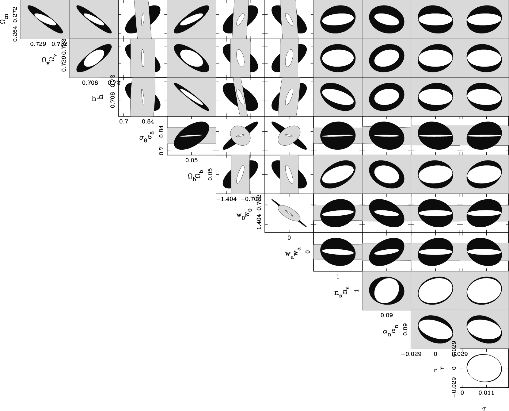
Figure 4: Expected marginal errors on cosmological parameters from Planck (dark), 3D weak lensing survey (light gray) and the combination (central, white). The survey covers $10,000$ square degrees to a median depth of $0.7$ in $5$ bands. Ellipses show the $1$-$\sigma$ errors for two parameters (68.3% confidence regions), marginalized over all other parameters.

3D weak lensing improves constraints on all the CMB cosmological parameters, in particular $\sigma_{8}$ whose constraint is improved by a factor of $14$. It is already well known that weak lensing can tightly constrain the ($\sigma_{8}$, $\Omega_{m}$) plane, using standard cosmic shear techniques (see Brown et al., 2003; Semboloni et al., 2006), 3D weak lensing constrains $\sigma_{8}$ in the same way by measuring the overall normalisation of the matter power spectrum. 3D weak lensing provides indirect (and slight) improvements on the constraints for the tensor to scalar ratio $r$ and the optical depth to last scattering $\tau$ through the intersection of the 3D weak lensing multi parameter ellipsoid with the CMB’s multi parameter constraint. Table 2 shows the $14$-month Planck constraints and the new combined constraints once 3D weak lensing is included. Note that results are presented for Universes which are not necessarily flat. In non-flat geometries the spherical Bessel functions $j_{\ell}(kr)$ should be replaced by ultra-spherical Bessel functions $\Phi^{\ell}_{\beta}(y)$. For the case considered here $\ell\gg 1$ and $k\gg$ (curvature scale)^-1 then $\Phi^{\ell}_{\beta}(y)\rightarrow j_{\ell}(kr)$ (Abbott and Schaefer, 1986; Zaladarriaga and Seljak, 2000). The expansion used is not ideal for non-flat Universes but should be an adequate approximation given current constraints on flatness.

Parameter	Planck only	Lensing only	Combined
$\Omega_{m}$	$0.0058$	$0.0500$	$0.0025$
$\Omega_{v}$	$0.0024$	$0.0795$	$0.0015$
h	$0.0088$	$0.0321$	$0.0051$
$\sigma_{8}$	$0.1002$	$0.0705$	$0.0073$
$\Omega_{b}$	$0.0011$	$0.3707$	$0.0007$
$w_{0}$	$0.5015$	$0.2843$	$0.1086$
$w_{a}$	$1.8618$	$1.1792$	$0.3947$
$n_{s}$	$0.0034$	$0.3852$	$0.0031$
$\alpha_{n}$	$0.0062$	$0.0576$	$0.0045$
$\tau$	$0.0079$		$0.0077$
$r$	$0.0208$		$0.0203$

Table 2: Improvements on CMB Planck one parameter 1-$\sigma$, constraints by adding 3D weak lensing from a 10,000 square degree lensing survey to a median depth of $z_{m}=0.7$.

5.3 Survey Optimization

For a given observing time, there will be an optimum depth of survey to minimize the statistical error on $w_{0}$ (or $w_{a}$). A very wide, shallow survey will yield poor cosmological constraints since the lensing signal is so small, whereas a very deep survey will also yield poor cosmological constraints because very little area can be covered, and the cosmic variance will be large. In addition, the distant galaxies will have shapes which are difficult to measure at high redshift. Here we explore the optimum median redshift using equation (36) keeping the time fixed, so that the area of the survey scales with median redshift as $A\propto z_{m}^{-4}$. The results are for $600$ nights on a 4m survey telescope with a 2 square degree field-of-view, where $z_{m}=0.70$ corresponds to $A=10,000$ square degrees. The results are shown in Figure 3.

The optimal median redshift for a $5$ band optical survey is $z_{m}=1.0$ with an area of $A=2400$ square degrees. The error is poor below $z_{m}\sim 1.0$ because the lensing signal becomes weaker, as the number of lensed background galaxies at high redshift decreases. For median redshifts above $z_{m}\sim 1.0$ the error is also poor as shot noise begins to dominate and the areal coverage becomes too small. We also investigate the effect of using $9$ and $17$ optical bands, keeping the median redshift and area fixed. We find that the marginal error does not substantially decrease. This is due to the combination of the lensing and CMB, the intersection of the ellipses in parameter space, remaining similar even though the lensing marginal errors on their own decrease with increasing bands. The extra bands might well be useful in the identification of outliers which we discuss in Section 5.5.2.

The optimal median redshift increases with the number of optical bands, a $17$ band optical survey has an optimal median redshift of $z_{m}=1.1$ with an area of $A=1640$ square degrees. Higher-$k$ modes are accessible due to the reduced damping effect of the photometric redshift error. In order to utilise these modes, the shot noise needs to be reduced, so the optimisation favours a slightly deeper survey with higher number density. This effect increases as the redshift uncertainty decreases.

Taylor et al. (2006) find that the optimal survey design for the geometric ratio method is $z_{m}=0.70$ and $A=10,000$ square degrees for a $5$ band photometric redshift survey on a $4$ metre telescope with a $2$ square degree field-of-view. So that the results presented here can be directly comparable with their results we shall adopt a fiducial survey design of $z_{m}=0.70$ and $A=10,000$ square degrees in $5$ bands from hereon; although it should be noted that given $600$ nights on such an instrument that an optimal survey design could improve the marginal errors on $w_{0}$ and $w_{a}$ using this method.

5.4 Weighting the data

We might expect that the cosmological parameter constraints could be improved if the more distant galaxies are given higher weight. We have not attempted a formal optimization, but show some results of experimental weighting schemes. We consider two weighting schemes $W(z)=z^{\alpha}$ and $W(z)=(1+z)^{\alpha}$. Figure 5 shows how the error on $w_{0}$ changes as the weighting scheme is changed. The figure shows the lensing-only marginal combined with a 14-month Planck prior on all parameters.

Figure 5: The variation in the lensing-only marginal error on $w_{0}$, as the weighting scheme is varied. The solid line is for $W(z)=z^{\alpha}$, the dashed line is for $W(z)=(1+z)^{\alpha}$; $\alpha$ is varied.

We show that the marginal error on $w_{0}$ is fairly insensitive to the weighting scheme employed. Furthermore using equal weighting is in fact the optimal strategy for a weighting functional form of this kind. This shows that the increase in the shot noise through the weighting of high redshift galaxies counteracts any improvement in the lensing signal, used to constrain $w_{0}$.

5.5 Optical and Infrared surveys

By combining a $5$ band optical survey with, for example, a $4$ band infrared survey the photometric redshift accuracy can decrease. Strategies such as this have the potential to be employed on future wide field surveys in an effort to improve cosmological parameter constraint. Here we parameterize the redshift error using

$$\sigma_{z}(z)=\sigma_{0}(1+z)$$ (37)

where a $5$ band optical survey can be approximately represented, see Figure 1, by $\sigma_{0}=0.05$. $\sigma_{0}=0.01$ corresponds to a $9$ band survey comprising of $5$ optical and $4$ infrared bands (Wolf, private communication). Note the distinction between this and the $9$ band optical (no infrared) survey considered in Section 5.3.

Figure 6 shows how the marginal error on $w_{0}$ varies with $\sigma_{0}$, here we fix the survey design to be $z_{m}=0.7$ and $A=10,000$ square degrees.

Figure 6: Marginal error on $w_{0}$ for different photometric redshift errors parameterized by $\sigma_{z}(z)=\sigma_{0}(1+z)$. These results include a $14$-month Planck prior.

We find that the marginal error on $w_{0}$ varies slowly between $0.01<\sigma_{0}<0.1$ and improves rapidly for $\sigma_{0}<0.01$. This turn-over corresponds to the point where the lensing pivot redshift error, see Section 5.7.1, becomes comparable to the CMB pivot redshift error. So, the marginal error of the combined constraint improves at a faster rate (as $\sigma_{0}$ decreases) after this point since the lensing constraint is improving $w_{0}$ and $w_{a}$ and lifting the CMB degeneracies further.

Figure 7: Marginal error on $w_{0}$ for different photometric redshift errors parameterized by $\sigma_{z}(z)=\sigma_{0}(1+z)$ for lensing (solid line) and a BAO experiment (dashed line) from survey of $z_{m}=0.70$ and $A=10,000$ square degrees. These results include a $14$-month Planck prior.

Figure 7 shows the marginal error from both lensing and BAO using the photometric redshifts from our fiducial survey. The treatment of a BAO experiment in a photometric redshift survey is discussed in Taylor et al. (2006). We find that BAO constraints do not significantly improve the $14$-month Planck prior for $\sigma_{0}>0.02$, and that for a $5$ band survey lensing provides much tighter constraints on the dark energy parameters. The dark energy constraints from lensing are less effected by the photometric damping of the radial wavenumber due to poor photometric errors than the BAO since lensing also gains dark energy information from geometric factor via the lensing effect. The BAO methodology on the other hand relies on a good measurement of the power spectrum which is restricted to low wavenumbers due to the photometric redshift errors. At low $\sigma_{0}$ the two methods provide complimentary constraints on $w_{0}$.

5.5.1 Bias in the photometric redshifts

As well as investigating the effect of varying the absolute values of the photometric errors, we would also like to investigate how a bias in the photometric redshift calibration effects the dark energy parameter estimation. Knox, Scoccimarro and Dodelson (1998), Kim et al. (2004) and Taylor et al. (2006) show how the bias $\delta\psi_{j}$ on a fixed model parameter $\psi_{j}$ is related to the marginal error on a (cosmological) parameter $\delta\theta_{i}$ by

$$\delta\theta_{i}=-[F^{\theta\theta}]_{ik}^{-1}F_{kj}^{\theta\psi}\delta\psi_{j}.$$ (38)

$F^{\theta\theta}$ is the cosmological parameter Fisher matrix and $F^{\theta\psi}$ is a pseudo-Fisher matrix between the measured and assumed parameters, when considering one parameter this is a column matrix.

We assume that there is some bias $z_{\rm bias}$ in the mean of the photometric redshifts in a given survey (see equation (16)) due to poor calibration of photometric redshifts with a spectroscopic training set. Marginalizing over all other parameters we find that

$$\delta w_{0}=-C_{\rm bias}\delta z_{\rm bias},$$ (39)

where $C_{\rm bias}$ is some constant. Following the arguments in Taylor et al. (2006) the number of galaxies requiring spectroscopic redshifts is

$$N_{\rm spec}=\left[\frac{C_{\rm bias}\sigma(z)}{\delta w_{0}}\right]^{2},$$ (40)

where the bias on $w_{0}$ is half the error $\delta w_{0}=0.5\Delta w_{0}$. We have found that $C_{\rm bias}\approx 1.2$ for 3D weak lensing. If $\sigma(z)\approx 0.1$ and we require $\Delta w_{0}\approx 0.01$ the number of spectroscopic redshift required is $N_{\rm spec}\approx 6\times 10^{2}$. This number is easily achievable using the current generation of spectrometers. The number of required spectroscopic redshifts is significantly smaller than the large number required for the geometric ratio test, for which $C_{\rm bias}\approx 9.0$ (e.g. Taylor et al., 2006) and tomographic methods (e.g. Hu and Jain, 2004), we attribute this difference to the binning procedure required in these methods. In binning the data any offset in the redshift estimation of a galaxy will create a discrepancy between the estimated and actual number of galaxies in a bin, and any derived quantities gained from them, for example the tangential shear behind a cluster. In this analysis any systematic offset in the galaxy population does not affect any derived quantities in this way but rather the whole shear field is offset in redshift, and galaxies are simply given a slightly increased weighting via $j_{\ell}$. Note that we consider only a single bias parameter, rather than the more complex behaviour allowed in Ma et al. (2005). However, it is the same model as used in our companion paper (Taylor et al., 2006) which shows more sensitivity to $z_{\rm bias}$.

Following the procedure outlined in Taylor et al. (2006) we also investigated the effect of an offset in the variance of the photometric redshift errors $\sigma_{z}(z)\rightarrow\sqrt{(\sigma_{z}^{2}(z)+\Delta\sigma_{z}^{2}(z))}$. We find that this effect is negligible for this analysis, so that the total bias due to photometric redshift errors is only dependent on the bias in the offset of the mean. We will explore fully marginalizing over nuisance parameters in a full Fisher analysis elsewhere.

5.5.2 The effect of outliers

In every photometric redshift survey there will be some galaxies in the sample for which an accurate photometric redshift cannot be assigned. To investigate the effect of these outliers on the dark energy parameter estimation we consider two galaxy populations, one with the original photometric redshift errors, see Section 4.1, and a second population with $\sigma_{z}^{p2}(z)=0.5$. We show the results in Figure 8, $A^{p2}$ is the proportion of the total galaxy population with $\sigma_{z}^{p2}=0.5$. We have considered three ways in which the outlying population could be dealt with, and how the effect of each of these methods varies with the proportion of the total population of outlying galaxies.

A population of outliers can either be discarded from the analysis completely or used in some way. The dashed line in Figure 8 shows the effect of discarding the sample, so that the surface number density of galaxies is decreased by $n_{0}\rightarrow n_{0}(1-A^{p2})$, but the photometric redshift error remains the same. To use the outliers either they can be treated as a separate population (solid line in Figure 8) or can be incorporated into a single population (dot-dashed line in Figure 8) in which case the overall photometric redshift is degraded to $\sigma_{z}(z)\rightarrow\sqrt{(1-A^{p2})[\sigma_{z}(z)]^{2}+A^{p2}[\sigma_{z}^{p2}(z)]^{2}}$ (see Blake & Bridle, 2005) where $\sigma_{z}(z)$ is the original photometric redshift error.

Figure 8: The effect of outliers with $\sigma^{p2}_{z}(z)=0.5$ on the marginal error in $w_{0}$ as a function of the proportion of outliers in the survey $A^{p2}$. The survey is a $5$ band survey of 10,000 square degrees to a median redshift of $z_{m}=0.7$, with a $14$-month Planck prior. The solid line shows the effect of treating the outliers as a separate population; the dashed line shows the effect of discarding the outliers; the dot-dashed line shows the effect of incorporating the outliers into a single galaxy population.

The effect of having outliers in the sample increases the marginal error on $w_{0}$ regardless of how they are treated, though the method is relatively insensitive to this effect. As expected using the outlying galaxies, and treating them as a separate population, increases the marginal error less than discarding the galaxies completely. By incorporating the galaxies into a single population the redshift error is degraded to such a degree that for a low proportion of outliers it is optimal to discard them, note the signal-to-noise for 3D weak lensing is proportional to $n_{0}$. For a high proportion it is optimal to include them somehow either into a single population or as two separate populations.

5.6 Scaling to other Surveys

Using the results presented in Sections 5.3 and 5.5 we can provide scaling relations in a similar way to Taylor et al. (2006). To scale these results to other weak lensing surveys, equation (36) should be used with a time calibration i.e.

$$\frac{T}{T_{0}}=\left(\frac{z_{m}}{z_{m0}}\right)^{4}\left(\frac{A}{A_{0}}\right)\left(\frac{D}{D_{0}}\right)^{-2}\left(\frac{fov}{fov_{0}}\right)^{-1}.$$ (41)

The subscript $0$ refers to the parameters time, median redshift and area of a survey on a telescope with certain diameter and field-of-view. The scaling applies between surveys with equal number of bands; for $5$ bands the Canada-France-Hawaii Telescope Legacy Survey (CFHTLS) can be used, while for $17$ bands COMBO-17 can be used. For other numbers of bands it can be naively assumed that the time for a given survey scales proportionally with the number of bands so that $T_{0}\rightarrow T_{0}N_{b0}/N_{b}$ where $N_{b}$ is the number of bands in the survey.

	CFHT	COMBO-17
D(m)	3.6	2.2
fov (sq deg.)	3	1
N (bands)	5	17
$z_{m}$	1.17	0.7
Area (sq.deg.)	170	1
T (nights)	500	6

Table 3: Default survey parameters for the 5-band CFHT Legacy Survey and the 17-band COMBO-17 survey.

For a flexible survey design the optimal median redshift of $z_{m}\approx 1.0$ is approximately insensitive to the number of bands, when combined with a Planck prior (see Figure 3). If the number of bands is $5$, $9$ or $17$ the appropriate line in Figure 3 then scales proportionally up (and down) with decreased (or increased) areal coverage from $2400$ square degrees, for a $5$ band survey i.e. $\Delta w_{0}(A)=(0.093)(A/2400)^{-1}$. If the number of bands is not shown in Figure 3 then Figure 6 can be used to find the minimum of the appropriate $\Delta w_{0}$ vs. $z_{m}$ line (at $z_{m}=0.7$). This can then be scaled for a differing areal coverage as before.

For a fixed survey of area $A$ and median redshift $z_{m}$ the error in Figure 3 for a given median redshift $\Delta w_{0}(z_{m})$ can be calculated using $\Delta w_{0}(A)=\Delta w_{0}(z_{m})(A/2400)^{-1}$. In scaling between bands a similar interpolation between Figure 3 and Figure 6 can be performed.

5.7 Constraining w(z) at higher redshifts

5.7.1 Pivot redshifts

The parametrization used for the dark energy equation of state encodes information on both the present day value of $w$ and its redshift evolution. By placing constraints on both $w_{0}$ and $w_{a}$ a region in the $w(z)$ vs. redshift coordinate system is constrained. Through the anti-correlation of $w_{0}$ and $w_{a}$ this constraint is minimized at a ‘pivot redshift’, the minimal error at this redshift being the pivot redshift error. The pivot redshift is schematically defined by the angle of the ellipse in the ($w_{0}$,$w_{a}$) plane, the error at this redshift being the width of the semi-minor axis of the ellipse.

Figure 9 shows the constraint on $w(z)=w_{0}+w_{a}(z/(1+z))$ as a function of redshift for our fiducial weak lensing survey. The highest accuracy on $w(z)$ occurs at the pivot redshift of $z=0.373$ with $\Delta w(z=0.373)=0.0175$.

Figure 9: Marginal error on $w(z)$ combined with a $14$-month Planck prior. The highest accuracy is achieved at the pivot redshift of $z=0.373$ with an error of $\Delta w(z=0.373)=0.0175$.

The pivot redshift of the CMB alone is $z=0.368$ with an error of $\Delta w(z=0.368)=0.0350$, the pivot redshift in this case is determined by the redshift at which the dark energy density begins to dominate over the matter density. The pivot redshift of 3D weak lensing alone is $z=0.208$ with an error of $\Delta w(z=0.208)=0.2018$ this is determined both by the redshift at which dark energy becomes dominant and the redshift at which the lensing signal is maximized.

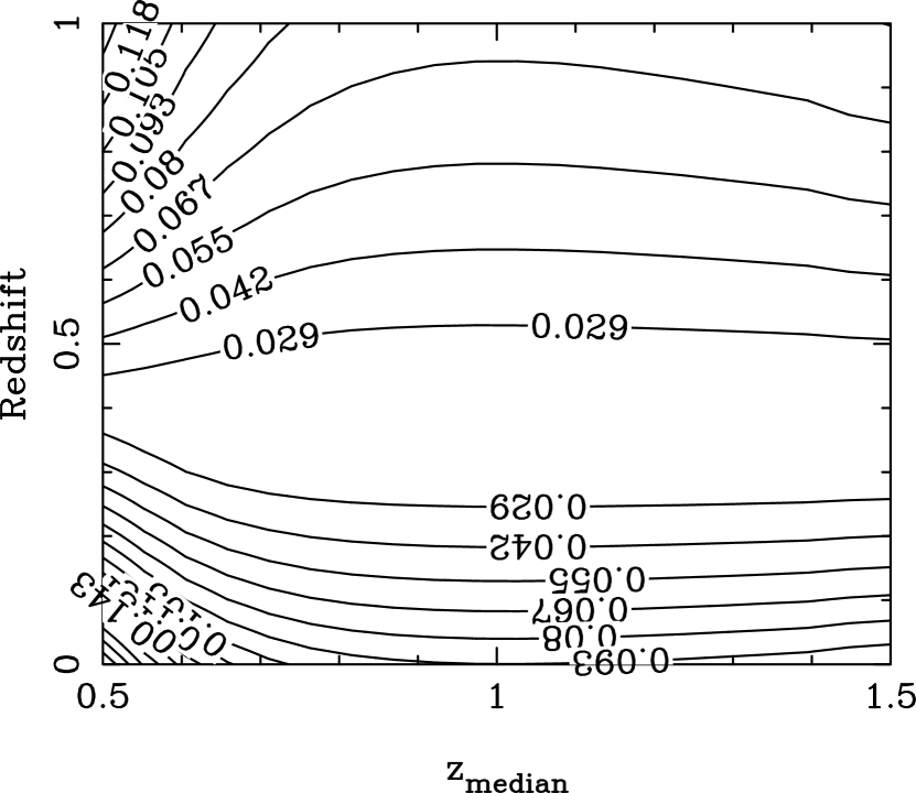
Figure 10: Marginal error on $w(z)$ combined with a $14$-month Planck prior as a function of median redshift. The contours are lines of equal marginal error the values of the contour given on the line.

Figure 10 shows how the error on $w(z)$ varies both with redshift and the median redshift of the survey. The line in Figure 9 can be found by tracing the $z_{m}=0.70$ line in Figure 10, the $5$ band line in Figure 3 can be found by tracing along the x-axis ($w(z)=w(0)=w_{0}$) in Figure 10. There is little sensitivity to the pivot redshift or the pivot redshift error on the survey design, this is due to the intersection of the 3D weak lensing constraint with the $14$-month Planck constraint remaining the same. This occurs because the pivot redshift of 3D weak lensing is a property of the cosmological dependence of the method not the survey design parameters, so that despite the marginal errors on $w_{0}$ and $w_{a}$ varying with the median redshift the orientation of the lensing ellipse, and hence its intersection with the $14$-month Planck ellipse, remains the same.

5.7.2 Figure of Merit

A ‘figure of merit’ has recently been introduced by the Dark Energy Task Force (DETF) (2006) (also see Linder, 2006; Taylor et al., 2006) which represents the area of the decorrelated ellipse constrained by a survey at the pivot redshift and can be written

$$\Delta w(z_{\rm pivot})*\Delta w_{a}.$$ (42)

In reference to Figure 9 the figure of merit quantifies both the minimal pivot redshift error and the redshift range over which the error in $w(z)$ is small; a wide and deep curve in Figure 9 would have a small figure of merit. Figure 11 shows how the figure of merit for a survey consisting of $600$ nights on a $4$ metre telescope with a $2$ square degree field-of-view varies with the median redshift of the survey.

Figure 11: The figure of merit (product of errors in $w(z_{\rm pivot})$ and $w_{a}$) as a function of median redshift for a $z_{m}=0.70$, $A=10,000$ square degree survey including a $14$-month Planck prior. Errors in $w_{0}$ and $w_{a}$ are marginalized over all other parameters. The solid line is for $5$-band photometric redshift survey, the dashed line for a $9$-band survey and the dot-dashed line for $17$-band survey. Note we assume shapes are not measurable beyond $z_{\rm max}=1.5$.

It can be seen that for a $5$, $9$ or $17$ band optical survey the optimal median redshifts are the same as when optimizing for $w_{0}$ alone, see Figure 3. It can be seen that the optimal median redshift in Figure 11 coincides with the widest point of the inner contour in Figure 10. The Figure of merit is shown for all considered experiments in Table 4.

6 Synergy of dark energy experiments

Here we present the results of comparing and combining 3D weak lensing with other dark energy probes. Combining probes, which use different cosmological effects to measure dark energy either through the growth of structure or geometric effects, will allow for cross checks to made. These cross checks may illuminate possible discrepancies between the two effects which could be important in determining the nature of dark energy. 3D weak lensing probes both the growth of structure via the matter power spectrum, and geometry through the lensing effect and the matter power spectrum.

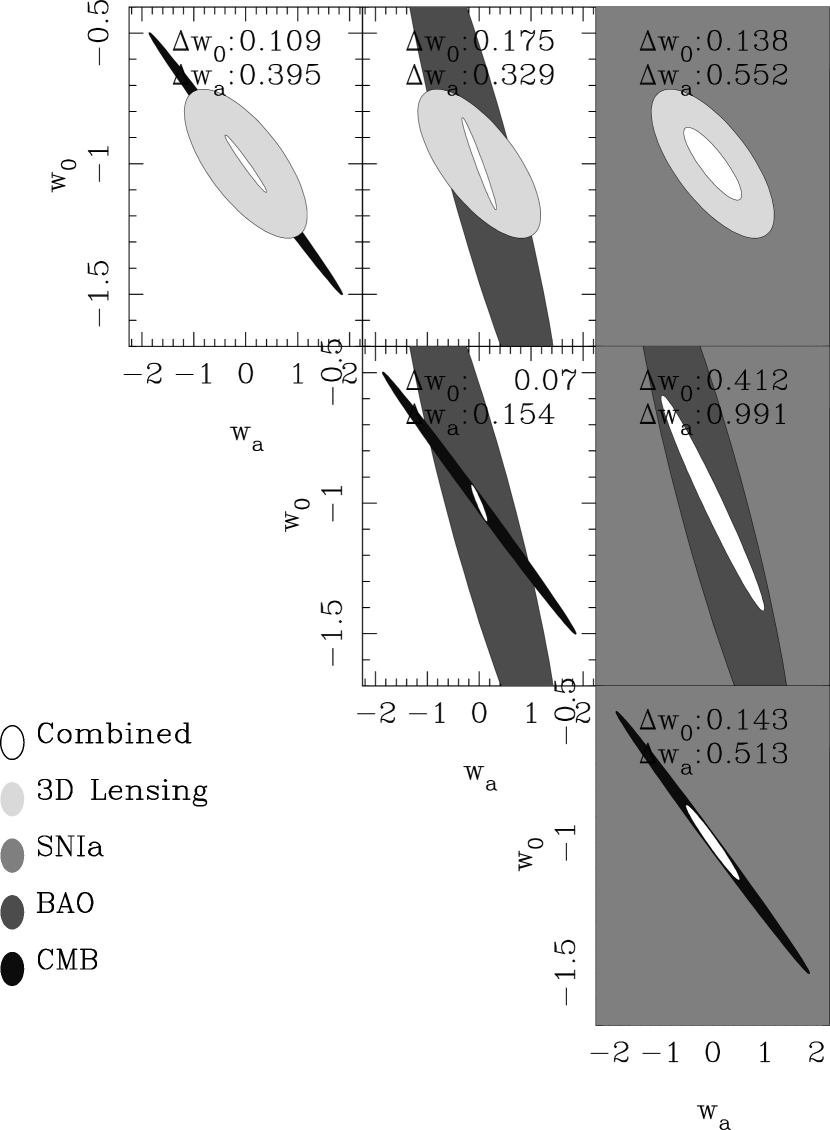
Figure 12: The combined marginal $w_{0}$, $w_{a}$ constraints for four individual experiments combined in pairs. The experiments are a darkCAM lensing experiment and a CMB 14-month Planck experiment, a BAO WFMOS experiment and a SNIa SNAP experiment. The dark ellipses in the diagonal panels is the CMB constraint; the small, light gray, ellipses along the top row of panels are the lensing constraint; the second lightest gray ellipses in the right-hand panels are the SNIa constraint; the broad darker gray ellipses in the top middle, right-hand middle and middle diagonal are the BAO constraint. The small white central ellipses are the combined constraints.

6.1 Comparing and combining with CMB, BAO and SNIA experiments

We consider the CMB, SNIa and BAO experiments as described in Section 5.1. In Figures 12, 13 and 14 the dark thin ellipse is the CMB constraint; the small lightest gray ellipse is the lensing constraint; the darker gray, almost vertical, broad ellipse is the BAO constraint; the very broad lighter gray ellipse is the SNIa constraint.

Figure 12 shows the combined two parameter $1$-$\sigma$ (68.3%) contours for all the possible pairs of experiments considered. In comparison with the other methods the 3D weak lensing constraint provides the smallest independent constraint. In combination the marginal errors so not vary largely between the different pairs. The BAO and CMB pair combination provides the smallest marginal errors through the unique degeneracy of the BAO ellipse providing a small intersection with the CMB. The SNIa constraint alone is poor although in combination with the other dark energy probes does provide an improvement on the marginal errors through the intersection of the constraints. The SNIa is also a purely geometric test, so that the combination with 3D weak lensing would provide an important cross check.

We combine combinations of three experiments in Figure 13. It can be seen, by comparing with Figure 12, that in adding further information from another experiment improves all the combined marginal errors. The largest improvements are gained by adding 3D weak lensing, or the CMB, to the pair combinations that do not include these probes. The smallest marginal errors are achieved by combining 3D weak lensing with the CMB and BAO. In combining 3D weak lensing with SNIa and BAO the dark energy constraints are comparable, or better than, each pair combination that includes the CMB constraint.

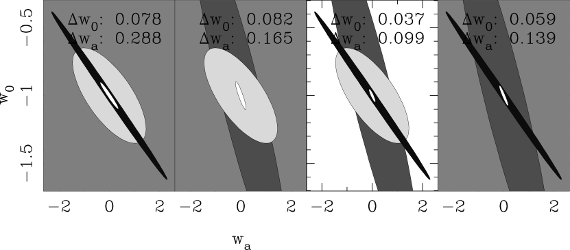
Figure 13: The combined marginal $w_{0}$, $w_{a}$ constraints for four experiments, combined three at a time. The experiments are a darkCAM lensing experiment, a CMB 14-month Planck experiment, a BAO WFMOS experiment and a SNIa SNAP experiment.

Finally the combination of all four of the dark energy probes is shown in Figure 14. By adding 3D weak lensing to the three experiment combination of CMB, BAO and SNIa the marginalized constraints are improved by a factor of $2$. The marginalized constraints in the combination of all four of the probes considered are

$$\Delta w_{0} = 0.035$$

$$\Delta w_{a} = 0.094,$$ (43)

with a pivot redshift error of

$$\Delta w(z=0.43)=0.0147.$$ (44)

Reducing the maximum $\ell$ to $2000$ increases these errors by approximately $0.01$ to $\Delta w_{0}=0.045$ and $\Delta w_{a}=0.105$.

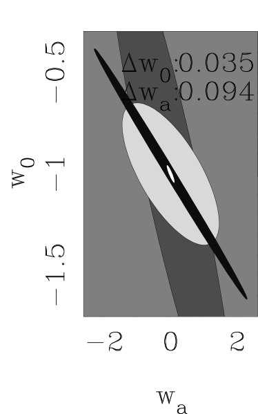
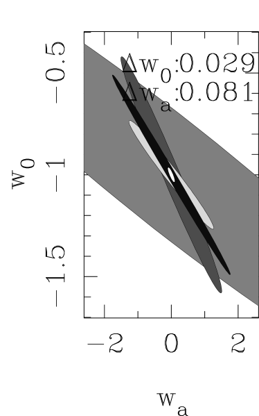
Figure 14: The left hand panel shows the combined marginal $w_{0}$, $w_{a}$ constraints for all four experiments combined allowing for fully open models, the right hand panel shows the combined marginal $w_{0}$, $w_{a}$ constraints for all four experiments combined, with the condition $\Omega_{m}+\Omega_{v}=1$ enforced. The experiments are a darkCAM lensing experiment and a CMB 14-month Planck experiment, a BAO WFMOS experiment and a SNIa SNAP experiment.

6.2 Complementary figures of merit and pivot redshifts

An illustrative way to present the information of pivot redshifts and the figure of merit of a dark energy probe, or combination of different probes, is to show how the figure of merit and the pivot redshift compare. We show this in Figure 15 by plotting the figure of merit for all the possible combinations of experiments against the pivot redshift of the combined constraint.

Figure 15: The figure of merit and pivot redshift for various experimental combinations. The combinations are labeled as L=3D weak Lensing, B=BAO, S=SNIa, C=CMB. Combinations of letters represent combinations of experiments.

In general the more experiments that are added in combination the smaller the figure of merit becomes. As more experiments are added in combination the pivot redshift converges to a single value. In combination with other experiments the BAO constraint creates a high pivot redshift, this is due to the redshift of the nearest bin at $z=1$. The 3D weak lensing constraint in combination creates a low $z\approx 0.4$ pivot redshift; this is due to the lensing pivot redshift dominating which is a symptom of the lensing signal maximizing at around that redshift. It can be seen from Figure 15 that there exists combinations, for example 3D weak lensing with the CMB (LC) and 3D weak lensing with BAO and SNIa (LSB), that have similar figures of merit but very different pivot redshifts. In using combinations such as these the $w(z)$ evolution could be constrained to a high degree over a large redshift range.

Survey	Area sqdeg	$z_{median}$	$N_{bands}$	$\Delta w_{0}$	$\Delta w_{a}$	$z_{\rm pivot}$	$\Delta w(z_{\rm pivot})$	$\Delta w(z_{\rm pivot})$$\Delta w_{a}$
Lensing
darkCAM + Planck	$10000$	$0.7$	$5$	$0.1082$	$0.3966$	$0.3681$	$0.0175$	$0.0069$
darkCAM + BAO darkCAM	$10000$	$0.7$	$5$	$0.2764$	$1.1207$	$0.2086$	$0.2004$	$0.0418$
darkCAM, 9 bands + Planck	$10000$	$0.7$	$9$	$0.1072$	$0.3895$	$0.3733$	$0.0173$	$0.0067$
SNAP Lensing + SNIa + Planck	$1000$	$1.38$	$5$	$0.0579$	$0.2322$	$0.3247$	$0.0112$	$0.0026$
All-Sky Space + Planck	$40000$	$1.0$	$9$	$0.0101$	$0.0406$	$0.3047$	$0.0342$	$0.0014$
darkCAM+Planck+BAO+SNIa	$10000$	$0.7$	$5$	$0.0350$	$0.0944$	$0.5011$	$0.0151$	$0.0014$
VST-KIDS+WMAP4	$1400$	$0.6$	$5$	$0.3405$	$1.0818$	$0.4378$	$0.0862$	$0.0933$
CFHTLS(Wide)+WMAP4	$170$	$1.17$	$5$	$0.2541$	$0.8145$	$0.4275$	$0.0711$	$0.0579$
CMB
4-year WMAP				$2.060$	$3.612$	$1.18$	$0.758$	$2.7379$
14-Month Planck				$0.501$	$1.873$	$0.367$	$0.035$	$0.0655$
BAO
BAO WFMOS+Planck	$2000$	$1.0$		$0.070$	$0.154$	$0.78$	$0.019$	$0.0029$
SNIa
SNIa SNAP+Planck				$0.142$	$0.513$	$0.37$	$0.028$	$0.0144$

Table 4: Expected marginal errors on cosmological parameters from 3D analysis of proposed weak lensing surveys. Note here $9$ bands refers to $5$ optical bands plus $4$ infrared.

6.3 Future lensing surveys

There are a number of current and planned imaging surveys for weak lensing which could be analyzed in 3D. The surveys vary in depth, areal coverage and number of bands, and illustrative errors are shown in the Table 4. Errors are marginalized. The surveys considered are: the Canada France Hawaii Legacy Survey (CFHTLS; Semboloni et al., 2006) which is ongoing; the VST (VLT Survey Telescope) public survey KIDS; SNAP (Supernova/Acceleration Probe; Aldering, 2005), and darkCAM on a $4$ metre telescope. We show the errors achievable with darkCAM combined with various different experiments. BAO darkCAM refers to using the photometric redshifts from darkCAM to measure BAO. VST-KIDS and CFHTLS have been combined with a $4$ year WMAP prior as Planck will not be contemporary with these surveys. Here 9 bands refers to a $5$ band optical survey with $4$ infrared bands as discussed in Section 5.5.

6.4 The effect of changing the fiducial dark energy model

Here we investigate the effect of the assumed fiducial dark energy cosmology on the marginal errors from our Fisher matrix calculations. The assumed cosmology has been a cosmological constant model with $w_{0}=-1$ and $w_{a}=0$. Figure 16 shows the two parameter $1$-$\sigma$ (68.3%) contours for various dark energy models in the ($w_{0}$, $w_{a}$) plane fully marginalized over other parameters. We consider two extreme examples, just allowable from current constraints: a SUGRA (Super Gravity) model proposed by Weller & Albrecht (2002) represented by $w_{0}=-0.8$ and $w_{a}=+0.3$; and a phantom model proposed by Caldwell et al. (2003) with $w_{0}=-1.2$ and $w_{a}=-0.3$. Despite the marginal errors from the dark energy experiments alone changing, the combined marginal error on $w_{0}$ is largely unaffected by the assumed dark energy model. The main difference is occurs on the error on $w_{a}$ which increases for all methods as its value becomes more negative. This is due to the fact that a negative $w_{a}$ represents a dark energy scenario in which the dark energy density was less in the past (increasing into the future); so that the effect of dark energy on the expansion rate on observed galaxies (in the past) is less in these scenarios (and similarly the opposite effect for a positive $w_{a}$). For the range of $w_{0}$ and $w_{a}$ allowed by current constraints the marginalized errors presented here should be robust to the actual nature of dark energy.

6.5 The effect of assuming flatness

Here we present the effect of assuming flatness in the parameter error estimation i.e. $\Omega_{v}=1-\Omega_{m}$. Figure 14 shows the two parameter $1$-$\sigma$ (68.3% contour) constraints for all four dark energy probes considered, see Section 5.1, in the ($w_{0}$, $w_{a}$) plane with the assumption that the Universe is flat. The CMB $14$-month Planck constraint does not considerably improve because the CMB puts a strong constraint on the overall geometry of the Universe, through the position of the first acoustic peak. The improvement in the SNIa constraint is most evident, since this dark energy probe is very sensitive to the overall geometry through the Hubble parameter (this is in agreement with Linder, 2005). The 3D weak lensing and BAO constraints also considerably improve, with the overall combined errors on the dark energy equation of state parameters being $\Delta w_{0}=0.029$ and $\Delta w_{a}=0.089$, a factor of $1.2$ less than the constraints considering fully open models. In assuming flatness the different dark energy probes still have unique and complimentary degeneracies in the ($w_{0}$, $w_{a}$) plane. The reduction in predicted errors, especially in the SNIa, 3D weak lensing and BAO experiments, show that the assumption of flatness can have an affect on parameter error estimation (this is in agreement with the affect of this assumption on weak lensing tomographic methods, see for example Knox, Song & Zhan, 2006). Given that some proposed dark energy models rely on modifications to the Friedmann equation in non-flat geometries it is prudent to calculate predicted parameter errors using fully open geometries.

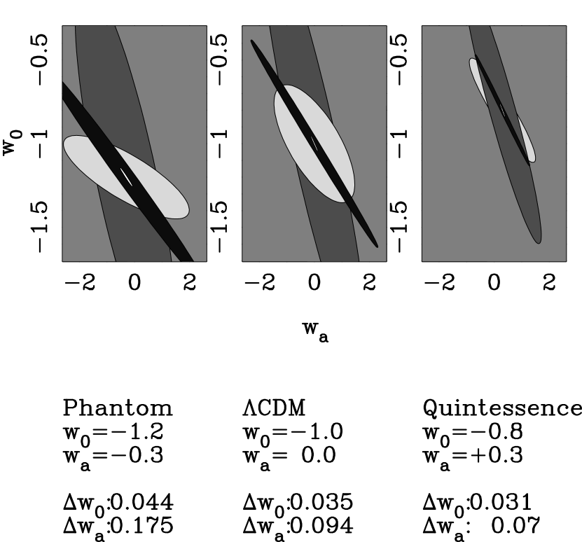
Figure 16: The two parameter $1$-$\sigma$ (68.3%) contours for various assumed fiducial dark energy models, for a 10,000 square degree survey to a median depth $z_{m}=0.7$, with a 14-year Planck prior, a BAO WFMOS prior and a SNIa SNAP prior. The errors quoted are the one parameter $1$-$\sigma$ marginal errors on $w_{0}$ and $w_{a}$. The dark thin ellipse is the CMB constraint; the small lightest gray ellipse is the lensing constraint; the darker gray, almost vertical, broad ellipse is the BAO constraint; the very broad light gray ellipse is the SNIa constraint. The small white central ellipses are the combined constraints.

7 Conclusions

In this paper we have presented a 3D weak lensing spectral method suitable for high-$\ell$ studies, and investigated how well 3D weak lensing surveys could determine the equation of state of dark energy. The accuracy which could be achieved if systematic errors can be controlled is impressively high, provided the surveys are analyzed in 3D: marginal statistical errors of $\Delta w_{0}=0.108$, on the current value of $w\equiv p/(\rho c^{2})$, and its evolution $w_{a}$ constrained to $\Delta w_{a}=0.397$ are possible with a 10,000 square degree survey in 5 bands to a median source depth of $z_{m}=0.7$. At a pivot redshift of $z=0.37$ such an experiment could constrain $w(z)$ to $\Delta w(z=0.37)=0.0175$. Such a survey is possible with darkCAM, in conjunction with data from the Planck satellite. Even without Planck, the accuracy from 3D weak lensing alone is still impressively high, and better than any other dark energy probe considered on its own. The fact that the physics of 3D weak lensing is well-understood, combined with the small statistical error forecasts, makes 3D weak lensing a formidable prospect for advancing cosmology in the next decade. The errors on $w$ are comparable to, but a little better than, predictions from tomography (Hu and Jain, 2004; Ishak, 2005). The constraints on $w(z)$ at the pivot redshift and the figure of merit, $\Delta w(z_{\rm pivot})*\Delta w_{a}$, of the experiments considered were also discussed.

We have investigated optimizing a wide field survey to measure the equation of state parameters $w_{0}$ and $w_{a}$ and found an optimal survey strategy of $z_{m}=1.0$ covering $2400$ square degrees for a $5$ optical band survey. We found that increasing the number of optical bands to $9$ or $17$ makes little difference to the marginal errors when the 3D weak lensing result is combined with a Planck prior. The effect of including infrared bands in a wide field survey was investigated by varying the photometric redshift error, it was found that adding $4$ infrared bands to a $5$ band optical survey improves the marginal constraints on $w_{0}$ slightly from $\Delta w_{0}=0.108$ to $\Delta w_{0}=0.097$.

Three alternative dark energy probes were considered: a Planck CMB experiment; a WFMOS BAO experiment and a SNAP SNIa experiment. All possible combinations of experiments were considered and the figure of merit and pivot redshifts of the combinations shown. In such a competitive environment 3D weak lensing places strong constraints on the dark energy parameters and in combination with other experiments provides a unique degeneracy in the ($w_{0}$,$w_{a}$) plane which is manifest as a strong constraint at a particular pivot redshift.

We have addressed the issues of biased photometric redshift estimates (e.g. Ma, Hu and Huterer, 2005) and show that the method is relatively insensitive to this. We also investigated the effect that a sample of outliers, with poor photometric redshift estimates, would have on the predicted marginal errors. The effect of outliers on the marginal error of $w_{0}$ is small although the way in which such a sample is treated is important.

We have not considered errors due to the intrinsic alignment of galaxies (Heavens, Refregier and Heymans, 2000; Croft and Metzler, 2000; Catelan, Kamionkowski and Blandford, 2001; Crittenden et al., 2001; Jing, 2002), as these may be reduced to a negligible level by removing pairs which are close in photometric redshifts (Heymans and Heavens, 2003; King and Schneider, 2002). This procedure has already been demonstrated in the analysis of the COMBO-17 data (Heymans et al., 2004). We have also not addressed other issues of systematics, such as optical distortions, or possible alignment of foreground galaxies with shear (Hirata and Seljak, 2004), which may be reduced using techniques such as template fitting (King, 2005). Nevertheless, the fact that the statistical errors are very small is very encouraging. Clearly to achieve the accuracies quoted here is going to be a formidable challenge for control of systematics, but at least the statistical error forecasts are small enough that the promise of accurate measurement of the equation of state of dark energy may be realized.

8 Acknowledgments

We would like to thank David Bacon and Graca Rocha for helpful discussions, Masahiro Takada for discussions concerning the CMB and BAO predictions, Chris Wolf for discussions concerning the photometric redshift error formalism. TDK acknowledges a PPARC studentship.

References

- [1] Abbott L., Schaefer R., 1986, ApJ, 308, 546
- [2] Aldering, G., 2005, NewAR, 49, 346
- [3] Bacon D., Refregier A., & Ellis R., 2000, MNRAS, 318, 625
- [4] Ballinger W., Heavens A., Taylor A., 1995, MNRAS, 276, 59
- [5] Bartelmann M. and Schneider P., 2001, Phys. Rep., 340, 291
- [6] Bassett B., et al., 2005, A&G, 46e, 26
- [7] Baugh C. and Efstathiou G., 1993, MNRAS, 265, 145
- [8] Bennett C. et al., 2003, ApJS, 148, 1
- [9] Bernstein G., 2005, astro-ph/0503276
- [10] Bernstein G., Jain B., 2004, ApJ, 600, 17
- [11] Blake C., Bridle S., 2005, MNRAS, 363, 1329
- [12] Brown M. et al., MNRAS, 314, 100
- [13] Castro P, Heavens A., Kitching T., 2005, Phys Rev D72, 023516 (astroph/0503479)
- [14] Catelan P., Kamionkowski M., Blandford R., 2001, MNRAS, 320, 7
- [15] Chevallier M., Polarski D., 2001, Int. J. Mod. Phy. D., 10, 213
- [16] Colless M., et al, 2001, MNRAS, 328, 1039
- [17] Crittenden R. et al., 2001, ApJ, 559, 552
- [18] Croft R. and Metzler C., 2002, ApJ, 545, 561
- [19] Croft R. et al. 2002, ApJ, 581, 20
- [20] DETF, 2006, http://www.nsf.gov/mps/ast/detf.jsp
- [21] Fisher K., Scharf C., Lahav O., 1994, MNRAS, 266, 219
- [22] Gnedin N., Hamilton A., 2002, MNRAS, 334, 107
- [23] Heavens A.F., 2003, MNRAS, 343, 1327
- [24] Heavens A., Refregier A., Heymans C., 2000, MNRAS, 319,649
- [25] Heavens A., Taylor A., 1995, MNRAS, 275, 483
- [26] Heymans C., Brown M., Heavens A., Meisenheimer K., Taylor A. Wolf C. 2004, MNRAS, 347, 895
- [27] Heymans C., Heavens A., 2003, MNRAS, 339, 711
- [28] Hirata C. & Seljak U. 2004, Phys. Rev. D204, 3056
- [29] Hoekstra H., Yee H., Gladders M., 2002, ApJ, 577, 595
- [30] Hoekstra H. et al., 2006, astroph, 0511089
- [31] Hu W., 1999, ApJ, 522, 21
- [32] Hu W., 2002, Phys. Rev. D66, 3515
- [33] Hu W. & Jain, B., 2004, Phys. Rev. D, 70, 043009
- [34] Hu W. & Tegmark M., 1999, ApJ, 514, L65
- [35] Huterer D., 2002, Phys. Rev. D, 65, 063001
- [36] Huterer D. et al., 2005, astroph/0506030
- [37] Ishak M., Hirata C., McDonald P. & Seljak U., 2004, Phys. Rev. D, 69, 083514
- [38] Ishak M., 2005, astro-ph/0501594
- [39] Jain B., Taylor A., 2003, Phys. Rev. Lett., 9, 1302
- [40] Jarvis M. et al., 2003, AJ, 125, 1014
- [41] Jarvis M., Jain B., Bernstein G. & Dolney D., 2005, astro-ph/0502243
- [42] Jing Y.P., 2002, MNRAS, 335, 89
- [43] Jungman G., Kamionkowski M., Kosowsky A., Spergel D., 1996, PhRvD, 54, 1332
- [44] Kaiser N., Wilson G., & Luppino G., 2000, astro-ph/0003338
- [45] King L., 2005, A&A, 441, 47
- [46] King L., Schneider P., 2002, A& A, 396, 411
- [47] Kim A., et al., 2004, MNRAS, 347, 909
- [48] Knox L., Scoccimarro R., Dodelson S., 1998, PhRvL, 81, 2004
- [49] Knox L., Song Y., Zhan H., 2006, astro-ph/0605536
- [50] Kuo C.L. et al., 2004, ApJ, 600, 32
- [51] Lamarre J. et al., 2003, NewAR, 47, 1017
- [52] Linder E., 2005, APh, 24, 391
- [53] Linder E., 2003, Phys. Rev. Lett., 90, 091301
- [54] Linder E., Jenkins A., 2003, MNRAS, 346, 573
- [55] Ma Z., Hu W., Huterer D., 2005, astroph/0506614
- [56] Peebles P., 1980, The Large-Structure of the Universe, Princeton University Press, Princeton
- [57] Pearson T., et al., 2003, ApJ, 591, 556
- [58] Percival W., et al., 2001, MNRAS, 327, 1297
- [59] Percival W., et al., 2004, MNRAS, 353, 1201
- [60] Ratra B., Peebles P., 1988, Phys. Rev. D37, 3406
- [61] Refregier, A., 2003 ARAA, 41, 645
- [62] Rhodes J. et al., 2004, ApJ, 605, 29
- [63] Riess A.G. et al. 2001, ApJ, 560, 49
- [64] Santos M., et al., 2003, MNRAS, 341, 623
- [65] Seljak U., Zaldarriaga M., 1996, ApJ, 469, 437
- [66] Semboloni E. et al., 2006, A&A, 452, 51S
- [67] Simon P., King L., Schneider P., 2004, A& A, 417, 873
- [68] Smith R. et al. 2003, MNRAS, 341, 1311
- [69] Song Y. & Knox L. 2004, Phys. Rev. D, 70, 063510
- [70] Spergel D. et al, 2003, ApJS, 148, 175
- [71] Spergel D. et al, 2006, astroph, 0603449
- [72] Tadros H. et al, 1995, MNRAS, 305, 527
- [73] Takada, M. & Jain, B. 2004, MNRAS, 348, 897
- [74] Takada M., White M., 2004, ApJL, 601, 1
- [75] Taylor A., 2005, ADS, pdus, confE, 28, http://www.noao.edu/meetings/subaru
- [76] Taylor A., Kitching T., Bacon D., Heavens A., 2006, astro-ph/0606416
- [77] Tegmark M., Taylor A., Heavens A., 1997, ApJ, 480, 22
- [78] Van Waerbeke, L. et al. 2000, A&A 358, 30
- [79] Verde L. et al., 2002, MNRAS, 335, 432
- [80] Wester W., 2005, ASPC, 339, 152
- [81] White, M. 2004, Astropart. Phys., 22, 211
- [82] Wittman D., Tyson J., Kirkman, D., Dell’Antonio I., & Bernstein, G. 2000, Nature, 405, 143
- [83] Wolf C., et al., 2001, A&A, 377, 442
- [84] Wolf C., et al., 2003, A&A, 401, 73
- [85] Wolf C., et al., 2004, A&A, 421, 913
- [86] Yèche C., et al., 2006, A&A, 448, 831
- [87] Zaldarriaga L., Seljak U., 2000, ApJS, 129, 431
- [88] Zhan H. & Knox L. 2004, Astrophys. J., 616, L75