Viscosity driven instability in rotating relativistic stars

Abstract

We investigate the viscosity driven instability in rotating relativistic stars by means of an iterative approach. We focus on polytropic rotating equilibrium stars and impose an $m=2$ perturbation in the lapse. We vary both the stiffness of the equation of state and the compactness of the star to study those effects on the value of the threshold. For a uniformly rotating star, the criterion $T/W$, where $T$ is the rotational kinetic energy and $W$ is the gravitational binding energy, mainly depends on the compactness of the star and takes values around $0.13\sim 0.16$, which differ slightly from that of Newtonian incompressible stars ($\sim 0.14$). For differentially rotating stars, the critical value of $T/W$ is found to span the range $0.17-0.25$. This is significantly larger than the uniformly rotating case with the same compactness of the star. Finally we discuss a possibility of detecting gravitational waves from viscosity driven instability with ground-based interferometers.

I Introduction

Stars in nature are usually rotating and subject to nonaxisymmetric rotational instabilities (see (Stergioulas, 2003), (Andersson, 2003), (Andersson and Comer, 2006) or (Villain, 2006) for recent reviews). An exact treatment of these instabilities exists only for incompressible equilibrium fluids in Newtonian gravity, (e.g. (Chandrasekhar, 1969; Tassoul, 1978; Shapiro and Teukolsky, 1983)). For these configurations, global rotational instabilities arise from non-radial toroidal modes $e^{im\varphi}$ ($m=\pm 1,\pm 2,\dots$) when $\beta\equiv T/W$ exceeds a certain critical value. Here $\varphi$ is the azimuthal coordinate and $T$ and $W$ are the rotational kinetic and gravitational binding energies. In the following we will focus on the $m=\pm 2$ bar-mode, since it is the fastest growing mode when the rotation is sufficiently rapid.

There exist two different mechanisms and corresponding timescales for bar-mode instabilities. Uniformly rotating, incompressible stars in Newtonian theory are secularly unstable to bar-mode formation when $\beta\gtrsim\beta_{\rm sec}\simeq 0.14$. This instability can grow in the presence of some dissipative mechanism, like viscosity or gravitational radiation, and the growth time is determined by the dissipative timescale, which is usually much longer than the dynamical timescale of the system. By contrast, a dynamical instability to bar-mode formation sets in when $\beta\gtrsim\beta_{\rm dyn}\simeq 0.27$. This instability is independent of any dissipative mechanism, and the growth time is the hydrodynamic timescale of the system.

There are two representative dissipative mechanisms that drive the secular bar mode instability, viscosity and the gravitational radiation, in the absence of thermal dissipation. The viscosity driven instability sets in when a mode has a zero-frequency in the frame rotating with the star (Roberts and Stewartson, 1963), and the first unstable mode in terms of $m$ is the $m=2$ bar mode. The quasi-static evolution of the star due to viscosity driven instability, which varies the circulation of the star, deforms the Maclaurin spheroid to the Jacobi ellipsoid in Newtonian incompressible stars. On the other hand, the gravitational radiation induced instability (Chandrasekhar, 1970; Friedman and Schutz, 1978) sets in when the backward going mode is dragged forward in the inertial frame (see (Stergioulas, 2003; Andersson and Comer, 2006; Villain, 2006; Schutz, 1987) for reviews), and the mode in terms of $m$ are all unstable when it exceeds a certain $m$. The quasi-static evolution of the star due to gravitational radiation induced instability, which varies the angular momentum of the star, deforms the Maclaurin spheroid to the Dedekind ellipsoid in Newtonian incompressible stars.

The viscosity driven instability, especially to determine the critical value either in an incompressible star or in an ellipsoidal equilibrium, has been studied in Newtonian gravity (Ipser and Mangan, 1981), in post Newtonian gravity (Shapiro and Zane, 1998; Di Girolamo and Vietri, 2002), and in full general relativity (Bonazzola, Frieben, and Gourgoulhon, 1996, 1998; Gondek-Rosińska and Gourgoulhon, 2002) by an ellipsoidal approximation (e.g. (Chandrasekhar, 1969)) or by an iterative evolution approximation (e.g. (Bonazzola, Frieben, and Gourgoulhon, 1996)), and shows that the viscosity drives the instability to higher rotation rates $\beta_{\rm sec}\gtrsim 0.14$ as the configurations become more compact. There is also a study of Newtonian compressible stars to determine the critical value of viscosity driven instability (Bonazzola, Frieben, and Gourgoulhon, 1996): It is found that the star becomes secularly unstable at $\beta_{\rm sec}\approx 0.135\pm 0.02$, depending on the stiffness of the polytropic equation of state.

The aim of the paper is twofold. One is to investigate the critical value of viscosity driven instability in the compressible stars rotating uniformly. The argument that the viscosity driven instability plays a role to deform a star from a Maclaurin spheroid to a Jacobi ellipsoid is only true in the absence of internal energy, since the total energy has a chance to transfer it to the internal energy without emission from the star (e.g. (Shapiro, 2004)). Here we assume that the cooling timescale of the star is shorter than the thermal heating timescale so that the thermal energy generated by viscosity is immediately radiated away. Therefore the picture of the deformation process due to viscosity is quite similar to the case of incompressible stars. The stars are usually considered as compressible bodies, and therefore it is worth to take such effect into account whether there is a significant change on the threshold. In this respect the present work extends that of Ref. (Gondek-Rosińska and Gourgoulhon, 2002) to the compressible case.

The other aim of the present work is to investigate the effect of differential rotation on the viscosity driven secular bar mode instabilities. For a strong viscosity or strong magnetic field circumstances, the star maintains uniform rotation. However, in nature the star may rotate differentially as the Sun. Stellar collapses and mergers may also lead to differentially rotating stars (e.g. (Ott et al., 2004)). For the coalescence of binary irrotational neutron stars (Shibata and Uryu, 2000, 2002; Shibata, Taniguchi, and Uryū, 2003), the presence of differential rotation may temporarily stabilize the “hypermassive” remnant, which constructs a differential rotation. Therefore it is also worth to take differential rotation into account to study viscosity driven instabilities in rotating relativistic stars.

This paper is organized as follows. In Sec. II we present the basic equations of our treatment of general relativity. We discuss our numerical results in Sec. III and in Sec. IV, focusing on the viscosity driven instability in uniformly and differentially rotating stars. In Sec. V we briefly summarize our findings. Throughout this paper, we use the geometrized units with $G=c=1$ and adopt polar coordinates $(r,\theta,\varphi)$ with the coordinate time $t$. Note that Latin index takes $(r,\theta,\varphi)$.

II Iterative evolution approach to determine the threshold of viscosity driven instability

II.1 Equilibrium configuration of rotating relativistic stars

We briefly introduce our basic approach to construct rotating relativistic stars and allow nonaxisymmetric deformation induced by “viscosity”. We introduce a nonaxisymmetric line element, when the azimuthal component $\varphi$ is separable in the metric (Chandrasekhar, 1983), in spherical coordinates $(t,r,\theta,\varphi)$ with a quasi-isotropic gauge (e.g. (Bonazzola et al., 1993; Gourgoulhon et al., 1999)) as

$$ds^{2} = -N^{2}dt^{2}+A^{2}(dr-N^{r}dt)^{2}+r^{2}A^{2}(d\theta-N^{\theta}dt)^{2}$$ (1)

$$+r^{2}\sin^{2}\theta B^{2}(d\varphi-N^{\varphi}dt)^{2},$$

where $N$ is the lapse, $N^{r}$, $N^{\theta}$, $N^{\varphi}$ correspond to the shift, $A$ and $B$ are the spatial metric functions. In the equilibrium state, we only take the azimuthal component of the shift $N^{\varphi}$, the lapse, and two spatial metric functions into account of the metric components. Note that all of them are functions of $r$ and $\theta$ only. Once we impose the nonaxisymmetric perturbation in the lapse, we take all the components of shift into account, and relax the dependence of the functions of ($r$, $\theta$) to ($r$, $\theta$, $\varphi$) for lapse and shift (Bonazzola, Frieben, and Gourgoulhon, 1998). In our present approach the nonaxisymmetric terms have been taken into account at least to the $1/2$ post-Newtonian order. Note that the spatial metric functions keep the functional dependence of ($r$, $\theta$) as those terms are considered as a higher post-Newtonian order which only enters in the order of $\varepsilon_{\rm amp}\times(M/R)\sim 10^{-6}$, where $\varepsilon_{\rm amp}$ is the amplitude of the perturbation we imposed in the lapse, $M$ the gravitational mass, $R$ the circumferential radius. It is therefore a good approximation to drop the nonaxisymmetric contribution from the spatial part of the metric. To summarize we compute the exact relativistic rotating equilibrium star and perturb the geometrical quantities in lapse and in shift, neglecting the azimuthal perturbation in the spatial metric.

We also adopt the maximal slicing condition, for which the trace of the extrinsic curvature $K_{ij}$ vanishes

$$K\equiv\gamma^{ij}K_{ij}=0.$$ (2)

The gravitational field equations (Einstein equations) for the six unknown functions $N$, $N^{r}$, $N^{\theta}$, $N^{\varphi}$, $A$, $B$ are written as (Bonazzola, Frieben, and Gourgoulhon, 1998)

$$\bar{\Delta}\,\nu\;=\;4\pi A^{2}[E+3P+(E+P)U_{i}U^{i}]+A^{2}K_{ij}K^{ij}$$

$$\quad-\bar{\nabla}_{i}\nu\,\bar{\nabla}^{i}(\nu+\beta),$$ (3)

$$\bar{\Delta}\,N^{i}+\frac{1}{3}\bar{\nabla}^{i}\bar{\nabla}_{j}N^{j}\;=\;-16\pi NA^{2}(E+P)U^{i}$$

$$\quad+NB^{-2}K^{ij}\bar{\nabla}_{j}(6\beta-\nu)\equiv J^{i},$$ (4)

$$\Delta_{2}\,[r\sin\theta(NB-1)]\;=\;16\pi r\sin\theta NA^{2}BP,$$ (5)

$$\Delta_{2}\,\zeta\;=\;8\pi A^{2}\,[P+(E+P)U_{i}U^{i}]+\frac{3}{2}A^{2}K_{ij}K^{ij}$$

$$\quad-\bar{\nabla}_{i}\nu\bar{\nabla}^{i}\nu,$$ (6)

where we introduced the auxiliary functions

$$\nu=\ln N,\quad\zeta=\ln(NA),\quad\beta=\ln B.$$ (7)

Note that $\bar{\nabla}_{i}$ denotes the covariant derivative in terms of a flat 3-metric, $\bar{\triangle}=\bar{\nabla}_{i}\bar{\nabla}^{i}$ the corresponding Laplacian, $\Delta_{2}$ is the 2-dimensional Laplacian, $U^{i}$ is the spatial component of 3-velocity

$$\Delta_{2}=\frac{\partial^{2}}{\partial r^{2}}+{1\over r}\frac{\partial}{\partial r}+{1\over r^{2}}\frac{\partial^{2}}{\partial\theta^{2}},$$ (8)

$$U^{r}=-\frac{N^{r}}{N},U^{\theta}=-\frac{N^{\theta}}{N},U^{\varphi}=\frac{1}{N}(\Omega-N^{\varphi}).$$ (9)

In Eqs. (3), (4), (5), and (6), $E$ and $U^{i}$ are the energy density and the 3-velocity, measured by the locally non-rotating observer: $E=\gamma^{2}[\rho(1+\varepsilon)+P)]-P$, $\gamma=[1-[A^{2}[(U^{r})^{2}+r^{2}(U^{\varphi})^{2}]+r^{2}\sin^{2}\theta B^{2}(U^{\varphi})^{2}]]^{-1/2}$, where $\rho$ is the comoving rest-mass density, $\varepsilon$ the specific internal energy, $P$ the pressure.

The equation for the shift,

$$\bar{\triangle}N^{i}+\frac{1}{3}\bar{\nabla}^{i}\bar{\nabla}_{j}N^{j}=J^{i},$$ (10)

can be further simplified by introducing a vector $W_{i}$ and a scalar $\chi$ according to

$$\triangle W_{i} = J_{i},$$ (11)

$$\triangle\chi = -J_{i}x^{i}.$$ (12)

The shift can then be computed from

$$N^{i}=\frac{7}{8}W^{i}-\frac{1}{8}[\bar{\nabla}^{i}\chi+\bar{\nabla}^{i}(W_{k}x^{k})],$$ (13)

and will automatically satisfy Eq. (10). The vector-type Poisson equation [Eq. (10)] for $N^{i}$ has hence been reduced to four scalar-type Poisson equations for $W^{i}$ and $\chi$.

Let us now discuss the matter part. We treat the matter as a perfect fluid, the energy momentum tensor of which is

$$T^{\mu\nu}=\rho\left(1+\varepsilon+\frac{P}{\rho}\right)u^{\mu}u^{\nu}+Pg^{\mu\nu},$$ (14)

where $u^{\mu}$ is the fluid 4-velocity. We adopt a $\Gamma$-law equation of state in the form

$$P=(\Gamma-1)\rho\varepsilon,$$ (15)

where $\Gamma$ is the adiabatic index. In the absence of thermal dissipation, Eq. (15) together with the first law of thermodynamics imposes a polytropic equation of state

$$P=\kappa\rho^{1+1/n},$$ (16)

where $n=1/(\Gamma-1)$ is the polytropic index and $\kappa$ a constant.

The relativistic Euler equation is described in axisymmetric stationary spacetime as

$$\frac{h_{,j}}{h}-\frac{u^{t}_{,j}}{u^{t}}+u^{t}u_{\varphi}\Omega_{,j}=0\quad(j=r,\theta),$$ (17)

where $h\equiv(1+\varepsilon+P/\rho)$ is the specific enthalpy. The Bernoulli’s equation is derived by integrating the relativistic Euler equation [Eq. (17)] as (see e.g. (Gourgoulhon, 2006))

$$H-K+R_{\rm rot}=C,$$ (18)

where

$$H \equiv \int\frac{dh}{h}=\ln h=\ln\left[1+\Gamma\varepsilon\right],$$ (19)

$$K \equiv \int\frac{du^{t}}{u^{t}}=\ln u^{t}=-\nu-\ln\gamma,$$ (20)

and $C$ is a constant of integration. We adopt two types of rotation profile, uniform and differential rotation, in this paper. For a uniformly rotating star, we simply set the rotational energy potential $R_{\rm rot}=0$ since $\Omega_{,j}=0$. For a differentially rotating star, we assume a specific type of rotation law as

$$u^{t}u_{\varphi}=A_{\rm rot}^{2}(\Omega_{\rm c}-\Omega),$$ (21)

where $\Omega_{c}$ is the central angular velocity, $A_{\rm rot}$ the degree of differential rotation, in order to integrate Eq. (17) analytically. In the Newtonian limit ($u^{t}\rightarrow 1$ and $u^{\varphi}\rightarrow\varpi^{2}\Omega$, where $\varpi$ is the cylindrical radius), the corresponding rotational profile reduces to

$$\Omega=\frac{A_{\rm rot}^{2}\Omega_{c}}{\varpi^{2}+A_{\rm rot}^{2}},$$ (22)

which is called $j$-constant rotation law. The rotational potential energy for this case is

$$R_{\rm rot}\equiv\int u^{t}u_{\varphi}d\Omega=-\frac{1}{2}A_{\rm rot}^{2}(\Omega_{c}-\Omega)^{2}.$$ (23)

The enthalpy is derived from the Bernoulli’s equation [Eq. (18)] as

$$H = H^{\rm max}+(K-K^{\rm max})-(R_{\rm rot}-R^{\rm max}_{\rm rot})$$ (24)

$$= \ln(1+\Gamma\varepsilon^{\rm max})+(\nu^{\rm max}-\nu)+(\ln\gamma^{\rm max}-\ln\gamma)$$

$$-(R_{\rm rot}-R^{\rm max}_{\rm rot}),$$

where $H^{\rm max}$, $K^{\rm max}$, $R^{\rm max}_{\rm rot}$ represents the values at the maximum enthalpy. The rotation law of the star [Eq. (21)] becomes

$$A_{\rm rot}^{2}(\Omega_{c}-\Omega)=\frac{r^{2}\sin^{2}\theta B^{2}(\Omega-N^{\varphi})}{N^{2}-r^{2}\sin^{2}\theta B^{2}(\Omega-N^{\varphi})^{2}}.$$ (25)

We also rescale the gravitational constant during the iteration process in order to determine the radius of the star (Bonazzola et al., 1993). Since the gravitational constant only enters through the matter of the star, we split the equation for lapse into two parts: One comes from the spacetime geometry and the other from the matter, and solve them independently ($\nu=\nu_{\rm q}+\nu_{\rm m}$, $\nu_{\rm q}$ is the contribution from the spacetime geometry and $\nu_{\rm m}$ the one from the matter). After that we set the equatorial surface in the computational domain and varies the gravitational constant (footnote, ) in the following:

$$G=\frac{(H^{\rm max}+\nu_{\rm q}^{\rm max}-\ln\gamma^{\rm max}+R^{\rm max}_{\rm rot})-(H^{\rm sur}+\nu_{\rm q}^{\rm sur}-\ln\gamma^{\rm sur}+R^{\rm sur}_{\rm rot})}{\nu_{\rm m}^{\rm sur}-\nu_{\rm m}^{\rm max}},$$ (26)

where $H^{\rm max}$, $\nu_{\rm q}^{\rm max}$, $\ln\gamma^{\rm max}$, $R^{\rm max}$ denotes the value at the maximum enthalpy, $H^{\rm sur}$, $\nu_{\rm q}^{\rm sur}$, $\ln\gamma^{\rm sur}$, $R^{\rm sur}$ denotes the value at the equatorial surface of the star, which are unknown in each iteration step.

In order to test our numerical code internally, we check the virial identities GRV2 (Bonazzola and Gourgoulhon, 1994) and GRV3 (Gourgoulhon and Bonazzola, 1994), the latter being a relativistic version of the classical virial theorem. The relative errors are defined by

$${\rm GRV2} = 1+\frac{\int_{0}^{\pi}d\theta\int_{0}^{\infty}rdr~{}\sigma_{\rm GRV2m}(r,\theta)}{\int_{0}^{\pi}d\theta\int_{0}^{\infty}rdr~{}\sigma_{\rm GRV2q}(r,\theta)},$$ (27)

$${\rm GRV3} = \frac{\int_{0}^{2\pi}d\varphi~{}\int_{0}^{\pi}\sin\theta d\theta~{}\int_{0}^{\infty}r^{2}dr~{}[\sigma_{\rm GRV3q}(r,\theta,\varphi)+\sigma_{\rm GRV3m}(r,\theta,\varphi)]}{\int_{0}^{2\pi}d\varphi\int_{0}^{\pi}\sin\theta d\theta\int_{0}^{\infty}r^{2}dr~{}\sigma_{\rm GRV3m}(r,\theta,\varphi)}.$$ (28)

where

$$\sigma_{\rm GRV2m}(r,\theta) = 8\pi A^{2}[P+(E+P)U_{i}U^{i}],$$ (29)

$$\sigma_{\rm GRV2q}(r,\theta) = \frac{3}{2}A^{2}K_{ij}K^{ij}-\bar{\nabla}_{i}\nu\bar{\nabla}^{i}\nu,$$ (30)

$$\sigma_{\rm GRV3m}(r,\theta,\varphi) = 4\pi A^{2}B[3P+(E+P)U_{i}U^{i}],$$

$$\sigma_{\rm GRV3q}(r,\theta,\varphi) = \frac{3}{4}A^{2}K_{ij}K^{ij}-\bar{\nabla}_{i}\nu\bar{\nabla}^{i}\nu$$ (32)

$$+\frac{1}{2}\bar{\nabla}_{i}\alpha\bar{\nabla}^{i}\beta.$$

Note that the two quantities GRV2 and GRV3, that should be identically 0 in the ideal equilibrium configuration, have already been rescaled by the typical source term of the equation, and therefore automatically defined as a relative error of our computation.

The gravitational mass $M$, proper mass $M_{p}$, total angular momentum $J$, rotational kinetic energy $T$, gravitational binding energy $W$ can be computed from

$$M = \int_{0}^{2\pi}d\varphi\int_{0}^{\pi}\sin\theta d\theta\int_{0}^{\infty}r^{2}dr~{}A^{2}B[N[E+3P$$

$$+(E+P)U_{i}U^{i}]+2r\sin\theta B(E+P)N^{\varphi}U_{i}U^{i}],$$

$$M_{p} = \int_{0}^{2\pi}d\varphi\int_{0}^{\pi}\sin\theta d\theta\int_{0}^{\infty}r^{2}dr~{}A^{2}B\gamma\rho,$$ (34)

$$J = \int_{0}^{2\pi}d\varphi\int_{0}^{\pi}\sin\theta d\theta\int_{0}^{\infty}r^{2}dr$$ (35)

$$\times r\sin\theta A^{2}B^{2}(E+P)U_{i}U^{i},$$

$$T = \frac{1}{2}\int_{0}^{2\pi}d\varphi\int_{0}^{\pi}\sin\theta d\theta\int_{0}^{\infty}r^{2}dr$$ (36)

$$\times r\sin\theta\Omega A^{2}B^{2}(E+P)U_{i}U^{i},$$

$$W = M_{p}+T-M.$$ (37)

Since we use a polytropic equation of state in the equilibrium, it is convenient to rescale all quantities with respect to $\kappa$. Since $\kappa^{n/2}$ has dimensions of length, we introduce the following nondimensional variables

$$\begin{array}[]{c c c}\bar{M}=\kappa^{-n/2}M,&\bar{R}=\kappa^{-n/2}R,&\bar{J}=\kappa^{-n}J,\\ \bar{T}=\kappa^{-n/2}T,&\bar{W}=\kappa^{-n/2}W,&\bar{\Omega}=\kappa^{n/2}\Omega.\end{array}$$ (38)

Henceforth, we adopt nondimensional quantities, but omit the bars for convenience (equivalently, we set $\kappa=1$).

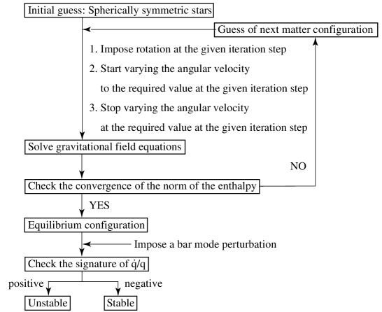
Figure 1: Sketch of the computational procedure to determine the stability of rotating stars.

Our computations have been made via a multi-domain spectral method (Bonazzola, Gourgoulhon and Marck, 1998). We have developed a code to implement this method by using the C++ library Lorene (lorene, ). The key advantage of the spectral method is that the required number of grid points to obtain a sufficiently high accuracy is quite small compared to the grid points in finite differencing, and the accuracy is guaranteed up to the round-off error in principle. Since this method is only applicable to smooth functions, we treat the discontinuity at the surface of the star by splitting the computational domain. Note that we introduce three computational domains to cover the space. The innermost domain covers the whole star, while the outermost one is compactified which allows to cover the space up to spatial infinity. We also use surface fitting method to split the domain at the surface of the star (Bonazzola, Gourgoulhon and Marck, 1998). This method works perfect until the equatorial surface of the star has a cusp, which happens when the uniformly rotating star approaches to the mass shedding limit, or the star is highly deformed from the sphere due to differential rotation.

II.2 Iterative evolution approach

We follow the iterative evolution approach (Bonazzola, Frieben, and Gourgoulhon, 1996, 1998) to investigate the viscosity driven instability in rotating relativistic stars. We particularly focus on the effect of relativistic gravitation for compressible fluids. The physical viewpoint of this approach is only shown in Newtonian incompressible star that to study the transition from a uniformly rotating axisymmetric body (Maclaurin spheroid) to a nonaxisymmetric body (Jacobi ellipsoid). According to Christodoulou et al. (1995), the above deformation process is driven by viscosity, since it only varies the circulation but keeps the other two conserved quantities, total energy and angular momentum, in the Newtonian incompressible star. The computational viewpoint of this approach is that instead of performing the time evolution of the star to investigate the stability of the star, we treat the iterative number as evolutional time and determine the stability of the star. The advantage of this approach is that there is no restriction to the evolutional timestep even in a high compactness star. Note that it is entirely difficult to study the secular instability in the explicit evolution scheme in full general relativistic hydrodynamics, since the restriction from the Courant timestep scales as $\sim(M/R)^{-1/2}$. The uncertain issue in this approach is that whether one can treat iterative number as evolutional time, and there is no relationship between each other in a mathematical sense. However there is a correspondence: In the Newtonian incompressible star, Gondek-Rosińska and Gourgoulhon (2002) investigate the difference between the exact critical value on the bifurcation point (e.g. (Chandrasekhar, 1969)) and find that it is within the round-off error.

Our computational study of the iterative evolution approach is divided into two stages; construction of a rotating equilibrium star and the determination of the viscosity driven bar mode stability of a rotating equilibrium star. To construct a rotating equilibrium star, we first construct a spherical star with given parameters of $\Gamma$ and $H_{\rm max}$, as an initial guess of the metric components and the matter profile. Next we solve gravitational field equations and determine the new matter profile for the next iteration step. During the iteration we impose rotation at the given iteration step, start varying the angular velocity to the given required value at the given iteration step, stop varying the angular velocity at the given required value at the given iteration step. We stop our iteration cycle when the relative error of the enthalpy norm between the previous step and the current step is within $1.0\times 10^{-7}$. We check the relativistic virial identity and the identity for all the equilibrium configuration and find that the relative errors of GRV2 and GRV3 are $\lesssim$ several $\times 10^{-4}$.

To determine the stability of rotating relativistic star driven by viscosity, we follow all the computational procedure to construct a rotating equilibrium star until we reach the relative error of the enthalpy norm at $1.5\times 10^{-7}$. At this iteration step, we put the following $m=2$ perturbation in the logarithmic lapse to enhance the growth of the bar mode instability as

$$\nu=\nu_{\rm eq}(1+\varepsilon_{\rm amp}\sin^{2}\theta\cos 2\varphi),$$ (39)

where $\nu_{\rm eq}$ is the logarithmic lapse in the equilibrium, $\varepsilon_{\rm amp}$ is the amplitude of the perturbation. We diagnose the maximum logarithmic lapse of the $m=2$ coefficients in terms of mode decomposition as

$$q={\rm max}~{}|\hat{\nu}_{2}|,$$ (40)

where

$$\nu=\sum_{m=0}^{\infty}\hat{\nu}_{m}e^{im\varphi}.$$ (41)

We also define the logarithmic derivative of $q$ in the iteration step ${\cal N}_{i}$ as

$$\frac{\dot{q}}{q}=\frac{q_{i}-q_{i-1}}{q_{i-1}},$$ (42)

where $q_{i}$ denotes $q$ at the iteration step ${\cal N}_{i}$. We determine the stability of the star in terms of viscosity driven instability as follows. When the diagnostic $q$ grows exponentially after we impose a bar mode perturbation in the logarithmic lapse, we conclude that the star is unstable. On the other hand when the diagnostic decays after we put a perturbation, the star is stable. More precisely, we monitor the derivative of $q$ after we impose a bar-mode perturbation. We conclude that the equilibrium star is unstable when the $\dot{q}/q$ settles down to a positive constant value, while stable to a negative constant value. Note that the existence of the plateau in $\dot{q}/q$ after the several iteration steps once we put a perturbation confirms us that we are in the linear perturbation regime, and therefore guarantees our choice of the perturbation amplitude we imposed ($\varepsilon_{\rm amp}$). Finally we determine the critical value of $T/W$ as the minimum one in the unstable branch. We also confirm our argument in all equilibrium stars that there is a continuous transition between stable and unstable stars as a function of $T/W$ in our model. We summarize our computational procedure in Fig. 1.

III Uniformly rotating stars

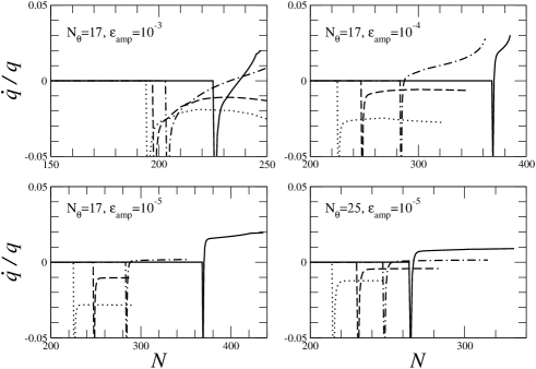
Figure 2: Diagnostic $\dot{q}/q$ as a function of iteration numbers ${\cal N}$ for sixteen different uniformly rotating stars of $\Gamma=2.3$ and $M/R=0.01$. Solid, dash-dotted, dashed, dotted lines denotes $T/W=(0.1306,0.1307,0.1308,0.1309)$ for $({\cal N}_{\theta},\varepsilon_{\rm amp})=(17,1.00\times 10^{-3})$, $T/W=(0.1309,0.1312,0.1313,0.1314)$ for $({\cal N}_{\theta},\varepsilon_{\rm amp})=(17,1.00\times 10^{-4})$, $T/W=(0.1309,0.1312,0.1313,0.1314)$ for $({\cal N}_{\theta},\varepsilon_{\rm amp})=(17,1.00\times 10^{-5})$, and $T/W=(0.1306,0.1307,0.1308,0.1310)$ for $({\cal N}_{\theta},\varepsilon_{\rm amp})=(25,1.00\times 10^{-5})$, respectively.

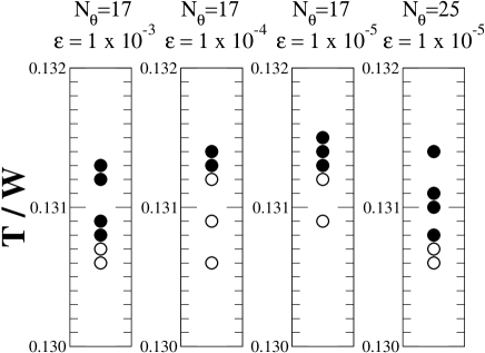
Figure 3: Stability of uniformly rotating stars of $\Gamma=2.3$, $M/R=0.01$ for four different parameters. Circle (open) and circle (filled) denotes stable and unstable to viscosity driven bar mode perturbation respectively. We fix the compactness for each parameter up to four digits. Note that there is a monotonic transition from stable to unstable when increasing $T/W$.

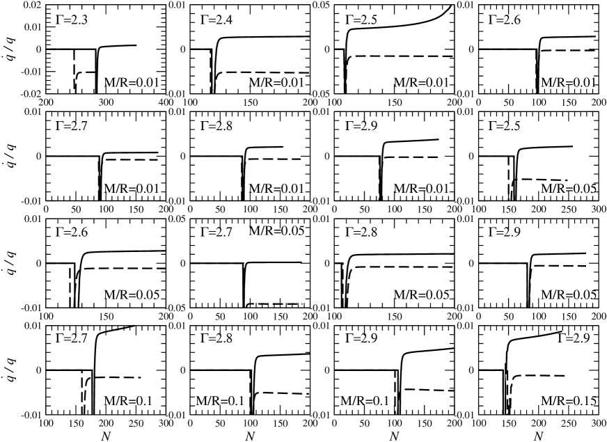
Figure 4: Diagnostic $\dot{q}/q$ as a function of iteration steps ${\cal N}$ for sixteen different uniformly rotating stars. Solid and dashed lines denotes the unstable and stable stars respectively. Note that the $T/W$ for each stable star in the same compactness is $0.0001$ lower than the critical value of that of an unstable star (see Table 2).

Before studying the viscosity driven instability in uniformly rotating stars, we examine the dependence of the perturbation amplitude $\varepsilon_{\rm amp}$ and the collocation points on the critical value of viscosity driven bar mode instability $(T/W)_{\rm crt}$. Note that we introduce three domains to cover the whole space, and each domain has a relationship of ${\cal N}_{r}=2{\cal N}_{\theta}-1$ and ${\cal N}_{\varphi}=4$, where ${\cal N}_{r}$, ${\cal N}_{\theta}$, ${\cal N}_{\varphi}$ represents the collocation points for the radial direction, the polar angle, the azimuthal angle, respectively.

First we vary the amplitude $\varepsilon_{\rm amp}$ in the range between $1.00\times 10^{-3}$ – $1.00\times 10^{-5}$. We show the diagnostic $\dot{q}/q$ in Fig. 2. The general picture of $\dot{q}/q$ in our computation is composed of three stages: (1) $\dot{q}/q=0$ (2) Sudden change in $\dot{q}/q$ at a certain iteration step (3) Continuous smooth function. (1) represents the stage of constructing the axisymmetric rotating equilibrium configuration. Since we solve the equations in the axisymmetric spacetime, there is no non-axisymmetric contribution in this stage and therefore both $q$ and $\dot{q}/q$ are $0$ up to numerical error. (2) represents a reaction due to a sudden imposition of a bar-mode perturbation in the logarithmic lapse. The quantity $\dot{q}/q$ should drastically change at this iteration step. (3) represents the post-perturbation stage, which determines the stability of the equilibrium star. When $\dot{q}/q$ takes a positive value after a certain iteration step we conclude that the equilibrium star is unstable, while takes a negative value stable. Note that it is in the linear perturbation regime when $\dot{q}/q$ takes a constant value after the perturbation. Therefore the solid and dash-dotted lines in Fig. 2 are stable while dash and dotted lines are unstable (plotted in Fig. 3). The diagnostic $\dot{q}/q$ suggests us to impose the amplitude below $1.00\times 10^{-4}$, since there is no plateau for the case of ${\cal N}_{\theta}=17$, $\varepsilon_{\rm amp}=1.00\times 10^{-3}$ in the stable star (Fig. 2). We also check whether we have a continuous transition from the stable star to the unstable one in terms of $T/W$ (Fig. 3), and confirmed that there exists a minimum $T/W$ in the unstable stars. We determine the minimum value as $(T/W)_{\rm crt}$. The monotonic increase of the final value of $\dot{q}/q$ as increasing $T/W$ (Fig. 2) also supports the previous statement. We find in Table 1 that the critical value of $T/W$ depends on the choice of $\varepsilon_{\rm amp}$ for only $0.4\%$, which means that we are in the high convergence level of the choice of $\varepsilon_{\rm amp}$.

Next we show our result of two different choices of the collocation points ${\cal N}_{\theta}=17$ and $25$ in Table 1, and find that the critical $T/W$ depends on the choice of ${\cal N}_{r}$ and ${\cal N}_{\theta}$ only for $0.4\%$. This means that we are also in the high convergence level in the choice of collocation points. Therefore we briefly estimate that our accuracy level of the critical value of $T/W$ is $\lesssim 1\%$. Hereafter we choose the parameter sets $\varepsilon_{\rm amp}=1.00\times 10^{-5}$ and ${\cal N}_{\theta}=17$ to determine the critical value of viscosity driven instability in uniformly rotating stars.

Table 1: Dependence of critical $T/W$ on the amplitude $\varepsilon_{\rm amp}$ and on the collocation points in uniformly rotating stars of $\Gamma=2.3$, $M/R=0.01$.

$\varepsilon_{\rm amp}$	${\cal N}_{\theta}$	$(T/W)_{\rm crt}$
$1.00\times 10^{-3}$	$17$	$0.1308$
$1.00\times 10^{-4}$	$17$	$0.1313$
$1.00\times 10^{-5}$	$17$	$0.1313$
$1.00\times 10^{-5}$	$25$	$0.1308$

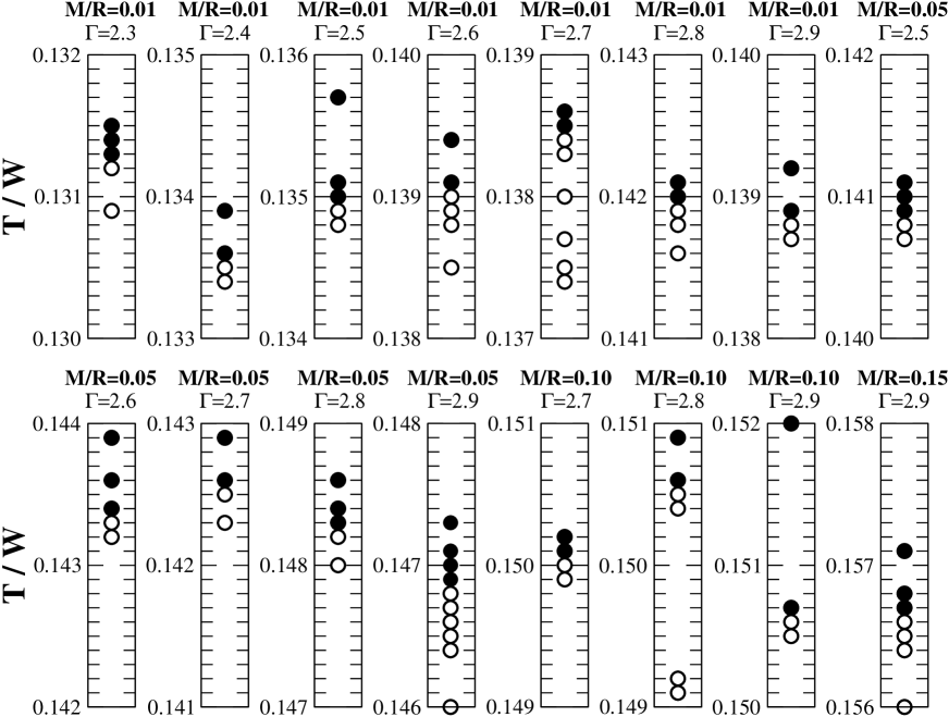
Figure 5: Stability of uniformly rotating stars for sixteen different parameters. Circle (open) and circle (filled) denotes stable and unstable to viscosity driven bar mode perturbation respectively. We fix the compactness for each parameter up to four digits. Note that there is a monotonic transition from stable to unstable when increasing $T/W$.

After we determine our choice of $\varepsilon_{\rm amp}$ and the collocation points, we study the critical value of $T/W$ of the viscosity driven instability in uniformly rotating stars. We show the diagnostic of the two closest star to the critical value of $T/W$ for sixteen different parameters in Fig. 4. Note that there is a clear plateau after we put a perturbation, and therefore we are in the linear perturbation regime. We also study the stability of the stars in terms of $T/W$ (Fig. 5) and determine the critical values of instability, which are summarized in Table 2 and in Fig. 6. We find that the relativistic gravitation stabilizes the star from viscosity driven instability, and that the critical value of $T/W$ for each compactness is almost insensitive to the polytropic $\Gamma$ of the equation of state. The Newtonian compressible calculation has been performed in Fig. 3 of Bonazzola, Frieben, and Gourgoulhon (1996) that the critical value of $T/W$ is $\sim 0.134$ which is not so sensitive to the variation of the polytropic $\Gamma$. Our computational results (Fig. 6) shows that the critical $T/W$ is $\sim 0.137$ for $M/R=0.01$ , $\sim 0.145$ for $M/R=0.05$, $\sim 0.150$ for $M/R=0.1$, $\sim 0.157$ for $M/R=0.15$, respectively. The critical value of $T/W$ monotonically increases when increasing the compactness of the star, which means that the relativistic gravitation stabilizes the viscosity driven instability. Note that the $\Gamma$ below the smallest $\Gamma$ in each compactness of the star plotted in Fig. 6 represents that the star is stable up to the mass-shedding limit.

Table 2: Critical value of $T/W$ of viscosity driven instability in uniformly rotating relativistic stars

$\Gamma$	$R_{p}/R_{e}$	$H_{\rm max}$	$R$	$M$	$J$	$(T/W)_{\rm crt}$	$M/R$	GRV2	GRV3
$2.30$	$0.5276$	$9.199\times 10^{-3}$	$0.9323$	$0.009322$	$0.0002082$	$0.1313$	$0.009999$	$6.44\times 10^{-5}$	$-1.54\times 10^{-4}$
$2.40$	$0.5446$	$8.465\times 10^{-3}$	$0.7518$	$0.007518$	$0.0001400$	$0.1336$	$0.01000$	$3.22\times 10^{-5}$	$-9.60\times 10^{-5}$
$2.50$	$0.5526$	$8.002\times 10^{-3}$	$0.6322$	$0.006322$	$0.0001008$	$0.1350$	$0.01000$	$-3.78\times 10^{-5}$	$1.04\times 10^{-4}$
$2.60$	$0.5482$	$7.662\times 10^{-3}$	$0.5528$	$0.005528$	$7.904\times 10^{-5}$	$0.1391$	$0.01000$	$5.04\times 10^{-5}$	$-2.14\times 10^{-5}$
$2.70$	$0.5590$	$7.368\times 10^{-3}$	$0.4825$	$0.004825$	$6.057\times 10^{-5}$	$0.1385$	$0.01000$	$7.99\times 10^{-5}$	$-1.73\times 10^{-4}$
$2.80$	$0.5510$	$7.130\times 10^{-3}$	$0.4352$	$0.04352$	$5.023\times 10^{-5}$	$0.1420$	$0.01000$	$-1.24\times 10^{-5}$	$8.59\times 10^{-5}$
$2.90$	$0.5663$	$6.933\times 10^{-3}$	$0.3879$	$0.003879$	$3.966\times 10^{-5}$	$0.1389$	$0.01000$	$5.85\times 10^{-5}$	$-1.52\times 10^{-4}$
$2.50$	$0.5312$	$4.542\times 10^{-2}$	$0.8140$	$0.04071$	$0.001986$	$0.1409$	$0.05001$	$4.72\times 10^{-5}$	$-1.30\times 10^{-4}$
$2.60$	$0.5368$	$4.291\times 10^{-2}$	$0.7267$	$0.03633$	$0.0001616$	$0.1434$	$0.05000$	$5.04\times 10^{-5}$	$-4.94\times 10^{-5}$
$2.70$	$0.5486$	$4.090\times 10^{-2}$	$0.6513$	$0.03256$	$0.001306$	$0.1426$	$0.05000$	$7.01\times 10^{-5}$	$-1.64\times 10^{-4}$
$2.80$	$0.5380$	$3.951\times 10^{-2}$	$0.6089$	$0.03044$	$0.001171$	$0.1483$	$0.05000$	$-1.02\times 10^{-4}$	$1.34\times 10^{-4}$
$2.90$	$0.5471$	$3.820\times 10^{-2}$	$0.5586$	$0.02793$	$0.0009868$	$0.1469$	$0.05000$	$4.99\times 10^{-5}$	$-1.23\times 10^{-4}$
$2.70$	$0.5241$	$9.710\times 10^{-2}$	$0.7320$	$0.07319$	$0.005049$	$0.1501$	$0.09999$	$7.93\times 10^{-5}$	$-7.16\times 10^{-5}$
$2.80$	$0.5351$	$9.197\times 10^{-2}$	$0.6734$	$0.06735$	$0.004319$	$0.1506$	$0.1000$	$7.23\times 10^{-5}$	$-1.86\times 10^{-4}$
$2.90$	$0.5423$	$8.824\times 10^{-2}$	$0.6274$	$0.06274$	$0.003773$	$0.1507$	$0.1000$	$8.09\times 10^{-5}$	$-3.63\times 10^{-5}$
$2.90$	$0.5242$	$1.608\times 10^{-1}$	$0.6634$	$0.09957$	$0.008380$	$0.1567$	$0.1501$	$3.16\times 10^{-5}$	$-6.99\times 10^{-5}$

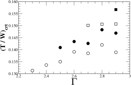
Figure 6: Critical value of $T/W$ as a function of $\Gamma$ for four different compactness of uniformly rotating stars (see Table 2). Circle (open), circle (filled), square (open), and square (filled) denotes the compactness ($M/R$) of $0.01$, $0.05$, $0.1$, and $0.15$, respectively. The star whose adiabatic index is $\Gamma_{\rm low}-0.1$, where $\Gamma_{\rm low}$ is the lowest $\Gamma$ of the unstable star in each compactness in the figure, is stable.

IV Differentially rotating stars

Next we follow the same approach to study the critical value of viscosity driven bar-mode instability in differentially rotating stars. We study two cases based on the variation of rotation profile during the iteration for differentially rotating stars. One is that we fix the rotation profile throughout the iteration. The physical timestep which corresponds to the iteration step is much shorter than the dynamical time in this case since the different fragments of the fluid in terms of a cylindrical radius move at different azimuthal speeds, and therefore the trace shows a spiral structure. The other is to change the rotation profile throughout the evolution. Since we mimic the model that the viscosity changes the rotation profile, the total angular momentum is approximately conserved throughout the process. We use the same collocation points as in the case of uniformly rotating stars.

First we show the case of fixed rotation profile throughout the evolution. The diagnostic in Fig. 7 shows that there exists a critical value of viscosity driven instability. Note that the plateau at the late stage of the iteration clearly shows that we are in the linear perturbation regime. We also monitor the stability of differentially rotating stars in terms of different $T/W$ in Fig. 8. We find a monotonic transition from a stable star to an unstable star as a function of $T/W$, which guarantees the determination of critical value of $T/W$ as a minimum $T/W$ in the unstable stars. We summarize our finding in Table 3.

We find the following two issues in the critical value of $T/W$. One is that relativistic gravitation also stabilizes differentially rotating stars from the viscosity driven instability. The above statement also holds in uniformly rotating incompressible relativistic stars and in uniformly rotating compressible relativistic stars, and therefore we find that this statement is quite general one. The other is that differential rotation also stabilize the star from the viscosity driven instability. The critical value of $T/W$ is $0.13\sim 0.16$ for a uniformly rotating star, while $0.18\sim 0.25$ for a differentially rotating stars with moderate degree of differential rotation.

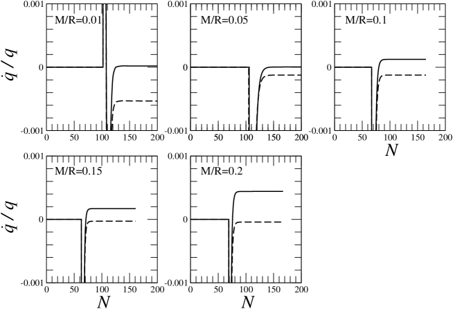
Figure 7: Diagnostic $\dot{q}/q$ as a function of iteration steps ${\cal N}$ for five different differentially rotating stars. Solid and dashed lines denotes the unstable and stable stars respectively. Note that the $T/W$ for each stable star in the same compactness is $0.0001$ lower than the critical value of that of an unstable star (see Table 3).

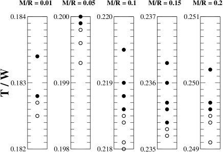
Figure 8: Stability analysis of differentially rotating stars for five different parameters. Circle (open) and circle (filled) denotes stable and unstable to viscosity driven bar mode perturbation respectively. We fix the compactness for each parameter up to four digits. Note that there is a monotonic transition from stable to unstable when increasing $T/W$.

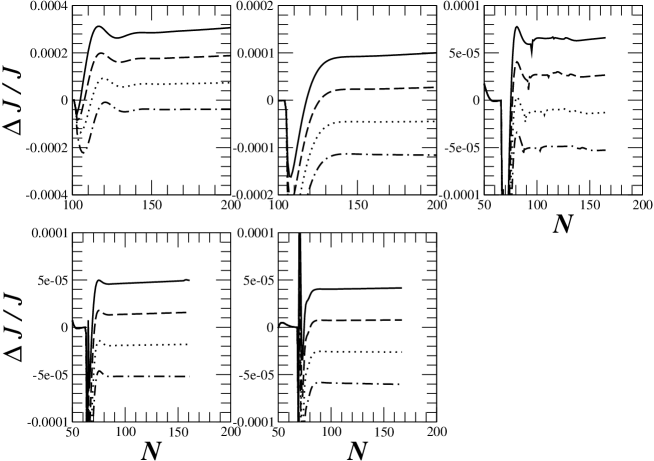
Figure 9: Relative deviation of the total angular momentum between two successive steps in the iteration process, as a function of the step number ${\cal N}$. Solid, dashed, dotted, dash-dotted lines represent $\varepsilon_{\rm omg}=(0.5,0.6,0.7,0.8)\times 10^{-4}$ for $M/R=0.01$ and $T/W=0.1828$, $\varepsilon_{\rm omg}=(0.8,0.9,1.0,1.1)\times 10^{-4}$ for $M/R=0.05$ and $T/W=0.1999$, $\varepsilon_{\rm omg}=(1.1,1.2,1.3,1.4)\times 10^{-4}$ for $M/R=0.1$ and $T/W=0.2186$, $\varepsilon_{\rm omg}=(1.0,1.1,1.2,1.3)\times 10^{-4}$ for $M/R=0.15$ and $T/W=0.2354$, and $\varepsilon_{\rm omg}=(0.9,1.0,1.1,1.2)\times 10^{-4}$ for $M/R=0.2$ and $T/W=0.2496$, respectively.

Table 3: Critical value of viscosity driven instability in differentially rotating relativistic stars. We choose $\Gamma=2$ polytropic equation of state and the degree of differential rotation as $\hat{A}=1$.

$R_{p}/R_{e}$	$H_{\rm max}$	$R$	$M$	$J$	$(T/W)_{\rm crt}$	$M/R$	GRV2	GRV3
$0.4458$	$7.594\times 10^{-3}$	$1.978$	$0.01978$	$0.01165$	$0.1828$	$0.01000$	$-2.03\times 10^{-6}$	$2.28\times 10^{-6}$
$0.3985$	$3.830\times 10^{-2}$	$1.894$	$0.09468$	$0.01315$	$0.1999$	$0.05000$	$3.92\times 10^{-6}$	$4.92\times 10^{-4}$
$0.3820$	$7.492\times 10^{-2}$	$1.758$	$0.1758$	$0.03565$	$0.2186$	$0.1000$	$3.88\times 10^{-7}$	$-4.52\times 10^{-6}$
$0.3457$	$1.116\times 10^{-1}$	$1.609$	$0.2414$	$0.06025$	$0.2354$	$0.1500$	$-1.93\times 10^{-5}$	$-9.03\times 10^{-6}$
$0.2982$	$1.581\times 10^{-1}$	$1.455$	$0.2910$	$0.08210$	$0.2496$	$0.2000$	$-3.63\times 10^{-6}$	$-1.55\times 10^{-5}$

Next we study the variation of the rotation profile since viscosity also takes a significant role to change it. The timescale between the change of angular velocity profile and the growth of the viscosity driven bar-mode are in the same order in low viscosity approximation, we should check whether our result is significantly affected by the change of the rotation profile of the star. In order to mimic this idea, we vary the parameter of the degree of differential rotation slightly after we impose a perturbation in the following manner:

$$A_{\rm rot}^{-1}=A_{\rm rot}^{-1~{}\rm(eq)}[1-\epsilon_{\rm rot}({\cal N}-{\cal N}_{\rm ptb})],$$ (43)

where $\epsilon_{\rm rot}$ is the degree of the variation of the rotation profile we set to $1.0\times 10^{-4}$, ${\cal N}$ the iteration number, ${\cal N}_{\rm ptb}$ the iteration number we impose the perturbation. Note that viscosity changes the rotation profile to the uniform one, we put negative sign in front of $\varepsilon_{\rm rot}$. Since the viscosity only affects the local interaction between the each fluid components, the total angular momentum is conserved even the viscosity takes the role. Therefore we also vary the central angular velocity $\Omega_{\rm c}$ in a following manner

$$\Omega_{\rm c}=\Omega_{\rm c}^{\rm(eq)}[1-\epsilon_{\rm omg}({\cal N}-{\cal N}_{\rm ptb})],$$ (44)

where $\epsilon_{\rm omg}$ is the degree of the variation of the central angular velocity in order to maintain the total angular momentum approximately constant. Note that we put negative sign in front of $\epsilon_{\rm omg}$ to play an appropriate role of the viscosity. In practice we vary $\epsilon_{\rm omg}$ in $0.1$ steps and choose the one that changes the angular momentum minimum at the given $\varepsilon_{\rm rot}$. For each case the relative change of the total angular momentum after we impose the perturbation is in the order of $\lesssim 10^{-5}$. We show the relationship between the relative change of the total angular momentum and $\epsilon_{\rm omg}$ for several cases in Fig. 9.

Taking into account of the change of rotational profile, we show our numerical results for the critical values in Fig. 10. We find that all the stars around the critical $T/W$ determined for a fixed rotation profile becomes unstable. In fact, the stage of $\dot{q}/q$ that corresponds to the plateau in Fig. 7 increases in Fig. 10. Therefore we estimate the relevant two timescales, growth of the bar mode due to viscosity and the variation time of the rotational profile due to viscosity, and compare them to discuss the condition to induce viscosity driven instability.

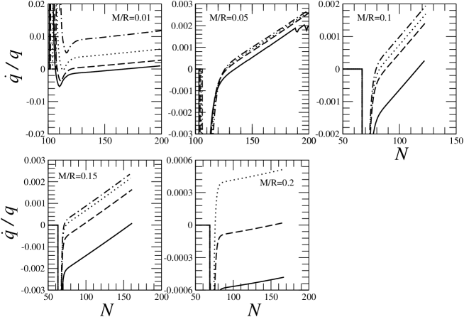
Figure 10: Diagnostic $\dot{q}/q$ as a function of iteration steps ${\cal N}$ for five different differentially rotating stars. Solid, dashed, dotted, and dashed line denotes $T/W=$ $(0.1825,0.1828,0.1834,0.1844)$ and $\varepsilon_{\rm omg}=0.8\times 10^{-4}$ for $M/R=0.01$, $T/W=$ $(0.1993,0.1996,0.1998,0.1999)$ and $\varepsilon_{\rm omg}=0.9\times 10^{-4}$ for $M/R=0.05$, $T/W=$ $(0.2180,0.2184,0.2185,0.2186)$ and $\varepsilon_{\rm omg}=1.3\times 10^{-4}$ for $M/R=0.1$, $T/W=$ $(0.2348,0.2352,0.2353,0.2354)$ and $\varepsilon_{\rm omg}=1.1\times 10^{-4}$ for $M/R=0.15$, and $T/W=$ $(0.2494,0.2495,0.2496)$ and $\varepsilon_{\rm omg}=1.0\times 10^{-4}$ for $M/R=0.2$, respectively. Note that $\dot{q}/q$ is always increasing around the critical value of $T/W$ in differentially rotating stars, which means the change of rotational profile due to viscosity unstabilizes the star.

If we assume that the bar grows exponentially throughout the iteration, the growth timescale of the bar is $(\dot{q}/q)^{-1}$. The value of $\dot{q}/q$ at the plateau in Fig. 7 represent the growth timescale. On the other hand, the change of the rotation profile due to viscosity changes the growth timescale of the bar, and therefore the derivative of the $\dot{q}/q$ represents the timescale of the change of rotation profile. We define those two timescales as

$$\tau_{\rm ang}=(\ddot{q}/q)^{-1/2},\quad\tau_{\rm bar}=(\dot{q}/q)^{-1}.$$ (45)

We summarize those two timescales from our computation in Table 4.

Table 4: Two timescales in differentially rotating stars extracted from our numerical results

$M/R$	$T/W$	$\tau_{\rm ang}$ [$\Delta{\cal N}$]	$\tau_{\rm bar}$ [$\Delta{\cal N}$]
$0.01$	$0.1825$	$1.8\times 10^{2}$	$-6.1\times 10^{2}$
$0.01$	$0.1828$	$1.7\times 10^{2}$	$5.1\times 10^{4}$
$0.01$	$0.1834$	$1.3\times 10^{2}$	$3.0\times 10^{2}$
$0.01$	$0.1844$	$8.1\times 10^{1}$	$1.1\times 10^{2}$
$0.05$	$0.1993$	$1.7\times 10^{2}$	$-1.7\times 10^{3}$
$0.05$	$0.1996$	$1.6\times 10^{2}$	$-2.7\times 10^{3}$
$0.05$	$0.1998$	$1.6\times 10^{2}$	$-8.1\times 10^{3}$
$0.05$	$0.1999$	$1.6\times 10^{2}$	$3.1\times 10^{5}$
$0.10$	$0.2180$	$1.6\times 10^{2}$	$-6.6\times 10^{2}$
$0.10$	$0.2184$	$1.6\times 10^{2}$	$-2.6\times 10^{3}$
$0.10$	$0.2185$	$1.5\times 10^{2}$	$-8.1\times 10^{3}$
$0.10$	$0.2186$	$1.5\times 10^{2}$	$8.0\times 10^{3}$
$0.15$	$0.2348$	$2.0\times 10^{2}$	$-4.8\times 10^{2}$
$0.15$	$0.2352$	$2.0\times 10^{2}$	$-1.7\times 10^{3}$
$0.15$	$0.2353$	$1.9\times 10^{2}$	$-3.4\times 10^{4}$
$0.15$	$0.2354$	$1.9\times 10^{2}$	$5.9\times 10^{3}$
$0.20$	$0.2494$	$8.1\times 10^{2}$	$-1.8\times 10^{3}$
$0.20$	$0.2495$	$8.5\times 10^{2}$	$-2.4\times 10^{4}$
$0.20$	$0.2496$	$7.7\times 10^{2}$	$2.3\times 10^{3}$

These two timescales can also be derived analytically in Newtonian gravity. The azimuthal component of the Newtonian Navier-Stokes equation is

$$\frac{\partial\Omega}{\partial t}=\frac{\nu}{\varpi^{3}}\frac{\partial}{\partial\varpi}\left(\varpi^{3}\frac{\partial\Omega}{\partial\varpi}\right),$$ (46)

where $\nu$ is a shear viscosity. We assume the time dependence of the angular velocity as $\Omega(t)=\Omega_{\rm eq}e^{-i\sigma t}$ at the derivation from the equilibrium due to viscosity, the timescale to change the angular velocity profile to the uniform rotation is

$$\tau_{\rm ang}=\sigma^{-1}=\frac{(\varpi^{2}+d^{2})^{2}}{8d^{2}\nu}>\frac{d^{2}}{8\nu}=\frac{R^{2}}{8\nu}\frac{\Omega_{c}}{\Omega_{c}-\Omega_{s}},$$ (47)

where $\Omega_{\rm s}$ is the equatorial surface angular velocity. Note that we adopt the $j$-constant rotational profile to the angular velocity (Eq. [22] in Newtonian gravity). The $e$-folding time of a compressible uniformly rotating star (Eq. [A20] of Ref. (Lai and Shapiro, 1995)) based on the Navier-Stokes equation is

$$\tau_{\rm bar}=\frac{\kappa_{n}R^{2}}{5\nu}\frac{\beta_{\rm sec}}{\beta-\beta_{\rm sec}},$$ (48)

where $\kappa_{n}$ is a structure constant depends on the polytropic index (Table 1 of Ref. (Lai, Rasio, and Shapiro, 1994); $\kappa_{n}=0.65345$ for $\Gamma=2$), $\beta_{\rm sec}$ a critical value of $\beta$ for the secular bar mode instability, $R$ is the equatorial radius of the star.

Based on the analytical estimation of the two timescales, the timescales used in our numerical results should be described as

$$\tau_{\rm ang} \approx \varepsilon_{\rm org}^{-1},$$ (49)

$$\tau_{\rm bar} \approx \varepsilon_{\rm org}^{-1}\left(\frac{\Omega_{c}-\Omega_{s}}{\Omega_{c}}\right)\left(\frac{\beta_{\rm sec}}{\beta-\beta_{\rm sec}}\right).$$ (50)

We confirm that differential rotation stabilizes the star from viscosity driven instability. Also Eq. (50) shows that the timescale of the bar becomes short when the rotational profile varies due to viscosity. The critical value of $T/W$ changes from the one computed in a fixed rotation profile, but the deviational ratio of $T/W$ is roughly the same order as the one of rotational profile, which means $\approx\varepsilon_{\rm org}$.

V Conclusions

We have studied the viscosity driven instability in both uniformly and differentially rotating polytropic star by means of iterative evolution approach in general relativity. We have focussed on the determination of the critical value of viscosity driven instability.

We find that relativistic gravitation stabilizes the star from the viscosity driven instability, with respect to Newtonian gravitation. Also the critical value is not sensitive to the stiffness of polytropic equation of state for a given compactness of the star. In a previous study devoted to compressible stars, Bonazzola, Frieben, and Gourgoulhon (1998) showed that relativistic gravitation does stabilize the uniformly rotating polytropic stars by investigating the mass-shedding sequence. Our study shows the concrete value of $(T/W)_{\rm crt}$ in the case of a uniformly rotating star. Also we have improved the numerical code with respect to the study (Bonazzola, Frieben, and Gourgoulhon, 1998) by making use of surface-fitted coordinates.

Besides we have found that differential rotation also stabilizes the star from the viscosity driven instability. If we fix the compactness of the star, we find a significant increase of the critical value of $T/W$, which supports the above statement. We also confirm this statement by changing the rotation profile due to viscosity and find that the differential rotation still stabilizes the threshold of viscosity driven instability. However to confirm the statement in differentially rotating stars, the study of other approaches such as implicit hydrodynamical evolution or eigenmode analysis should be necessary and helpful.

Finally let us mention the characteristic amplitude and frequency of gravitational waves emitted throughout the viscosity driven secular bar mode instability, which produces quasi-periodic gravitational waves detectable in ground based interferometers. The characteristic amplitude $h$ of gravitational waves estimated from the evolution of a Jacobi-ellipsoid to a Maclaurin spheroid is (Eq. [4.2] of Ref. (Lai and Shapiro, 1995))

$$h\approx 9.1\times 10^{-21}\left(\frac{30{\rm Mpc}}{d}\right)\left(\frac{M}{1.4M_{\odot}}\right)^{3/4}\left(\frac{R}{10{\rm km}}\right)^{1/4}f^{-1/5},$$ (51)

where $d$ is the distance to the source and the characteristic frequency $f=\Omega/\pi$ is $f\gtrsim 1000{\rm[Hz]}$, depending on $T/W$ of the star. Note that the frequency increases throughout this process. Although the frequency regime of the source is slightly higher than the best sensitivity regime of the ground based detectors to follow all the deformation process, we may have a chance to detect them when it happens in the Virgo cluster, for example.