Is There a Fundamental Line for Disk Galaxies?

Abstract

We show that there are strong local correlations between metallicity, surface brightness, and dynamical mass-to-light ratio within M33, analogous to the fundamental line of dwarf galaxies identified by Prada & Burkert (2002). Using near-infrared imaging from 2MASS, the published rotation curve of M33, and literature measurements of the metallicities of H II regions and supergiant stars, we demonstrate that these correlations hold for points at radial distances between 140 pc and 6.2 kpc from the center of the galaxy. At a given metallicity or surface brightness, M33 has a mass-to-light ratio approximately four times as large as the Local Group dwarf galaxies; other than this constant offset, we see broad agreement between the M33 and dwarf galaxy data. We use analytical arguments to show that at least two of the three fundamental line correlations are basic properties of disk galaxies that can be derived from very general assumptions. We investigate the effect of supernova feedback on the fundamental line with numerical models and conclude that while feedback clearly controls the scatter in the fundamental line, it is not needed to create the fundamental line itself, in agreement with our analytical calculations. We also compare the M33 data with measurements of a simulated disk galaxy, finding that the simulation reproduces the trends in the data correctly and matches the fundamental line, although the metallicity of the simulated galaxy is too high, and the surface brightness is lower than that of M33.

1. INTRODUCTION

Prada & Burkert (2002, hereafter PB02) recently found that the dwarf galaxies in the Local Group obey a puzzling correlation between mean metallicity and global dynamical mass-to-light ratio (M/L). By combining this relationship with the previously known trend of metallicity with central surface brightness (e.g, Phillipps, Edmunds, & Davies, 1990; Caldwell et al., 1998), PB02 demonstrated that all three parameters together form an even stronger relationship, which they labeled the fundamental line of dwarf galaxies. PB02 showed that the metallicity-M/L ratio correlation can be explained by a simple chemical enrichment model. In this model, galactic winds continuously remove the heavy elements formed in dwarf galaxies from their interstellar medium, and star formation in these galaxies ends when all of the gas has been blown out of the system. Because more metals are retained by more massive galaxies (which have lower mass-to-light ratios) this model is able to reproduce the observed metallicity-M/L relationship. However, the model does not make clear why including surface brightness as a third parameter improves the correlation, and it is also surprising that variables such as morphological type and star formation history have no apparent effect on the fundamental line. PB02 proposed that feedback from star formation or supernovae could be involved in regulating the fundamental line, and Dekel & Woo (2003) and Tassis et al. (2003) used analytical arguments and simulations, respectively, to show that supernova feedback can produce relationships like the fundamental line, but additional work is needed to improve this understanding.

Two natural questions arise from these previous investigations of the fundamental line. First, does the fundamental line hold for massive galaxies as well as dwarfs? Galactic winds and supernova feedback should operate less effectively in larger galaxies as a result of their deeper potential wells, so if either of these processes is the primary mechanism responsible for setting the fundamental line correlations, the fundamental line should not be the same for massive systems. Second, is the fundamental line a local law as well as a global one? If not, it would be puzzling that all dwarf galaxies know to follow the relationship globally without having any corresponding correlations on smaller scales. The data to test the fundamental line locally in dwarfs do not yet exist, because spatially resolved metallicity measurements have not been obtained, and few dSph and dE galaxies have well-resolved kinematics either. Answering either of these questions with existing data therefore requires us to move to more massive galaxies.

In order to explore further the nature of the fundamental line, we consider the case of a well-resolved disk galaxy with known variations of its metallicity, surface brightness, and mass-to-light ratio with radius. The best example of a galaxy with these necessary characteristics is M33. We will address the following questions with this study. 1) Does the fundamental line hold locally, at every point within a galaxy? 2) Do the parameters of the global and local (assuming one exists) fundamental lines agree? 3) What is the origin of the fundamental line? 4) Can simulations of galaxy formation reproduce the fundamental line?

In this paper, we use several recently published data sets to investigate the local fundamental line in M33. In the next section, we combine a deep Two Micron All Sky Survey (2MASS) mosaic of M33 (Block et al., 2004), high resolution CO and H I rotation curves (Corbelli, 2003; Corbelli & Salucci, 2000), and literature metallicity measurements to construct the necessary observational quantities. In §3 we perform fits to the various relationships between mass-to-light ratio, metallicity, and surface brightness, and in §4 we compare the locally determined fundamental line of disk galaxies to the fundamental line of dwarf galaxies, give derivations of two of the fundamental line relationships, and discuss the implications of our findings. We also use the recent $\Lambda$CDM disk galaxy simulation by Robertson et al. (2004) to test how accurately current simulations can reproduce the properties of galaxies and we employ additional toy models of galaxy formation to understand the impact of feedback on the fundamental line. We briefly summarize our results and conclude in §5.

2. DATA AND ANALYSIS

Of the observations required for this study, the most restrictive is the large sample of accurate metallicity measurements as a function of radius. Many nearby galaxies have high-quality rotation curves and deep optical imaging, although $K_{s}$ band imaging to the depth of the 2MASS images (see §2.2) is less common. However, only two galaxies — M101 (Kennicutt, Bresolin, & Garnett, 2003) and M33 — have measured abundances for more than $\sim 10$ H II regions. Because M101 is a massive galaxy (and therefore more dynamically dominated by baryons), is nearly face-on (making its kinematics more difficult to measure accurately), and is significantly lopsided (indicating a possible recent interaction), it is not an ideal target for this study, and we instead focus exclusively on M33.

2.1. Abundances

Studying the fundamental line over a large range of galactic environments requires abundance measurements covering as wide a range of radii as possible. Because we will be comparing abundances to other local properties, it is important that we use a consistent abundance scale. We therefore limit our H II region sample to objects with directly-determined electron temperatures (although we do include CC93, the closest H II region to the center of M33, for which abundances were derived from strong-line model fitting by Vílchez et al. 1988). We also utilize abundances for M33 B supergiants, which have metallicities consistent with those of the H II regions in M33, although with slightly larger scatter.

The abundance of oxygen in the interstellar medium (ISM) and in the young stellar population of M33 has been sampled across the disk of the galaxy using both star-forming regions and young stars. We have compiled abundance data for 13 H II regions derived from optical spectroscopy (Smith, 1975; Kwitter & Aller, 1981; Vílchez et al., 1988) and ISO LWS spectroscopy (Higdon et al., 2003). The compilation of abundances for 13 bright M33 supergiants came from Monteverde et al. (1997), Urbaneja (2004), and Urbaneja et al. (2005). These works used quantitative spectroscopy of M33 supergiants, subsequently analysed with state of the art model atmospheres of massive stars. Combining these data sets yields 26 metallicity measurements in M33, spanning radii from 140 pc out to 6.2 kpc. The metallicity measurements employed in our study are plotted as a function of radius in Figure 1. Note that we assume a distance of 800 kpc throughout this paper (Lee et al., 2002; McConnachie et al., 2004), although some other recent determinations suggest a distance of more than 900 kpc (Kim et al., 2002; Ciardullo et al., 2004).

Figure 1.— Oxygen abundances as a function of radius in M33. The filled points represent abundance measurements from H II regions and the open points represent abundance measurements from B supergiants.

Abundance data for other astrophysical sources have been reported in the literature for M33: e.g., planetary nebulae (PN; Magrini et al., 2003, 2004) and supernova remnants (SNR; Blair & Kirshner, 1985); overall the PN and SNR abundances show a general agreement with the abundances derived for the H II regions (see Vílchez et al., 1988; Magrini et al., 2004; Stasińska et al., 2005). However, only small samples of these objects have been observed, and the scatter in the data is large, indicating that further observations are needed to understand how accurately they trace the present ISM abundances. Therefore, for the purposes of this paper we have not used PN and SNR data to trace the abundance gradient, though we point out that PN and (possibly also) SNR abundance results appear consistent with the data set used here.

2.2. 2MASS Images

In addition to providing relatively shallow near-infrared images of the entire sky, the 2MASS project also made deeper observations of several nearby galaxies. The deep exposures of M33 have integration times six times longer than the standard 2MASS data, so they reach $\sim 1$ mag fainter in surface brightness (Block et al., 2004). Tom Jarrett has kindly provided us with a mosaic of the individual images that covers the entire galaxy, with foreground stars and background (sky) variations removed.

$K_{s}$ band surface brightnesses at the position of each H II region and B star were measured by adding up the flux contained in circular apertures of radius 7″. The local surface brightnesses measured in this way are consistent with the azimuthally averaged surface brightness (see below) at the same radius within the uncertainties. Although the H II regions themselves contribute negligibly to the observed flux at this wavelength, in some cases a single star coincidentally located very close to the H II regions adds significantly to the flux, biasing the surface brightness high. To avoid this contamination, in such cases we instead measured the surface brightness in a blank region of sky a few arcseconds away.

To obtain deprojected galactocentric distances of the H II regions and B stars, we assumed a constant position angle of $22\arcdeg$ and a constant inclination angle of $50\arcdeg$ (see §2.3). The ellipses were centered on the galaxy nucleus at $01\mbox{${}^{h}$}33\mbox{${}^{m}$}50\fs 90$ $+30\arcdeg 39\arcmin 36\farcs 2$, which is consistent with the listed position of M33 in the 2MASS Extended Source Catalog (see also Jarrett et al., 2003). The surface brightness profile that we derive is displayed in Figure 2 along with an exponential disk fit. The large-scale background subtraction that was performed on the image makes accurate assessment of surface brightness errors extremely difficult. We therefore added a minimum uncertainty of 0.1 mag arcsec^-2 in quadrature to the measured Poisson uncertainties (T. Jarrett 2004, personal communication). Our fits to the surface brightness profile (see §2.3) yielded an extrapolated central surface brightness for the disk of $\mu_{K}=17.51\pm 0.06$ and a disk scale length of $5.86\arcmin\pm 0.28\arcmin$ (1.36 kpc). This value for the scale length is in agreement with the previous near-infrared photometric analysis by Regan & Vogel (1994), but the central surface brightness we measure is $\sim 0.15$ mag brighter, even after accounting for the different inclination angles. Because M33 is very extended compared to the largest near-infrared CCD mosaics currently available, determining an accurate photometric zeropoint for the surface photometry is quite difficult, which is likely the cause of the different central surface brightnesses derived by us and Regan & Vogel (1994). The imaging by Regan & Vogel (1994) did not reach the edge of the galaxy, suggesting that they may have derived an incorrect sky level, but the sky subtraction is sufficiently problematic that either or both works may have a systematic zeropoint offset of $\sim 0.15$ mag.

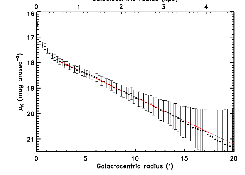
Figure 2.— $K$-band surface brightness profile of M33 from 2MASS data. The error bars represent formal statistical uncertainties from the isophotal fits, which clearly overestimate the true uncertainties. The solid red line shows the exponential disk fit to the surface brightness profile.

2.3. Rotation Curve

In order to calculate the dynamical mass of M33, we need a rotation curve. The best existing rotation curves of M33 are those constructed by Corbelli (2003) in CO and Corbelli & Salucci (2000) in H I, which are both consistent with the high-resolution CO observations of Engargiola et al. (2003). Corbelli & Salucci (2000) fit a tilted-ring model to the H I velocity field that they observed with the Arecibo telescope. They augmented their low resolution (beam FWHM of 3$\farcm$5 = 790 pc) data with interferometric observations near the center of the galaxy by Newton (1980) with a beam size of $47\times 93\arcsec$. The best-fitting model constructed by both sets of authors has a position angle (PA) of $\sim 22\arcdeg$ and an inclination angle of $\sim 50\arcdeg$ over the portion of the galaxy covered by the 2MASS images (both angles change slowly with radius, but for simplicity we ignore these variations). Although the near-infrared images clearly show that the central 20′ of M33 have a larger inclination angle (58$\arcdeg$) and a smaller PA (14$\arcdeg$), we use the kinematic values of these parameters for our surface photometry to maintain consistency between the photometry and the mass model.

Corbelli (2003) used a new CO map of M33 from the 14 m FCRAO telescope to confirm the accuracy of the H I data and further improve the angular resolution in the inner part of the galaxy. We use the CO data out to a radius of 6 kpc and the H I data at larger radii. The combined CO and H I rotation curve has a resolution element that ranges from 45″ to 3$\farcm$5 and features typical velocity uncertainties of $\sim 2$ km s^-1. The overall mass distribution of M33 is very well constrained by these data.

We construct a mass model of the galaxy assuming that it consists of a spherical dark matter halo and thin disks of gas and stars. The stellar surface density profile is derived from the 2MASS $K_{s}$ image with the IRAF task ellipse in the STSDAS package, and the atomic and molecular surface density profiles are taken from Corbelli & Salucci (2000) and Corbelli (2003), respectively. The rotation curves due to each of the baryonic components are determined directly from the surface density profiles by numerical integration using the NEMO software package (Teuben, 1995). The observed CO and H I surface density profiles extend out to a radius of 80′ (the edge of the rotation curve), but the stellar surface densities can only be measured out to 20′. To extend the rotation curve from the stellar disk out to larger radii, we extrapolate the stellar surface densities using the exponential disk fit from §2.2. We assume a maximal stellar disk, which for these data occurs at a stellar mass-to-light ratio of $\mbox{$M_{*}/L_{K}$}=0.51\mbox{$M_{\odot}/L_{\odot K}$}$. It is worth noting that this value is in agreement with the stellar M/L predicted from the galaxy color of $\mbox{$M_{*}/L_{K}$}=0.55\mbox{$M_{\odot}/L_{\odot K}$}$ (Bell & de Jong, 2001). The rotational velocities due to the dark halo are then calculated by subtracting in quadrature the rotation curves of the stellar and gaseous disks from the observed rotation curve (see Figure 3). To lessen the influence of small-scale bumps and wiggles and ensure that the dark matter rotation curve is monotonically increasing, we then replace the dark halo rotation velocities with a power law fit. We find that $v_{rot}\propto r^{0.53}$ provides an excellent fit to the data. Since the dark halo is assumed to be spherical, the mass profile of the dark matter is easily determined from its rotation curve.

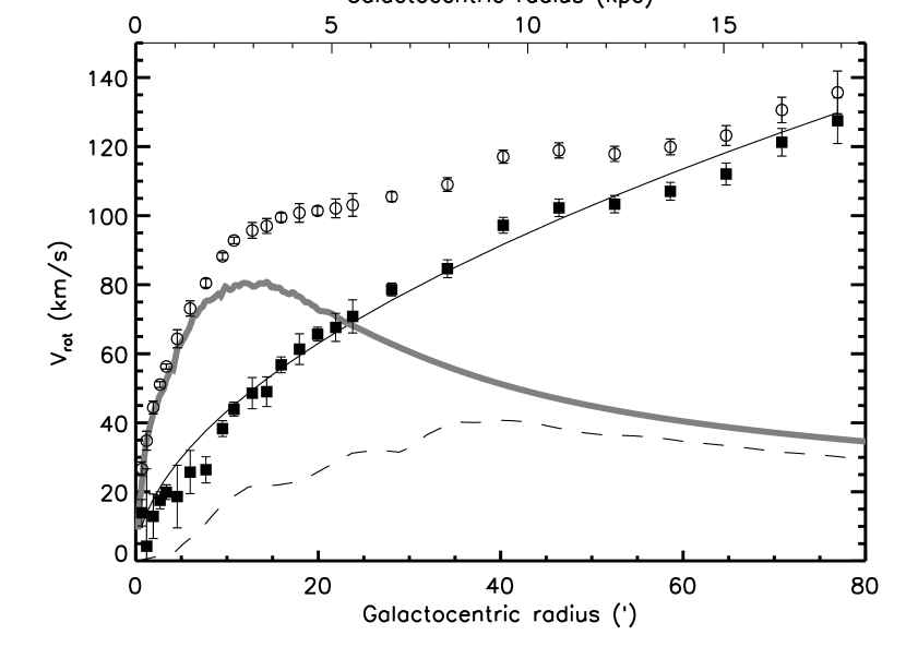
Figure 3.— Rotation curve of M33. The open circles are the CO and H I observations from Corbelli (2003) and Corbelli & Salucci (2000). The thick gray curve represents the rotation curve of the stellar disk (for a stellar mass-to-light ratio of $\mbox{$M_{*}/L_{K}$}=0.51\mbox{$M_{\odot}/L_{\odot K}$}$), the dashed black curve shows the rotation curve of the gas disk, and the black rectangles are the rotation curve of the dark matter halo after removing the contributions of the stars and gas. The thin black solid curve is a power law fit to the dark halo rotation curve.

To derive local values of the dynamical M/L, we divide each mass component into annuli and add up the total mass contained in each annulus. We divide up the light profile in the same way, and then take the ratio of the mass to the light in each annulus. This M/L profile can then be interpolated into a smooth function that gives the M/L at any radius. Note that unlike the surface brightness measurements, these mass-to-light ratios are not truly local measurements in the sense of being determined at a single position in the galaxy. Because of the nature of a rotation curve derived from a two-dimensional velocity field, the M/L values are necessarily azimuthally averaged quantities.

The uncertainties on the mass-to-light ratios that we derive deserve some further comment here (see also §3). Although the uncertainties on the rotation curve and the light profile of the galaxy are known, and therefore we can straightforwardly estimate the uncertainty on the integrated mass-to-light ratio interior to a particular radius, the uncertainty on the local mass-to-light ratio at any given radius is less well defined since it is effectively the ratio of differences between large numbers. Because the other galaxy properties that we are comparing with M/L are measured locally, it is important that we use local mass-to-light ratios instead of integrated ones, despite the potentially large uncertainties involved.

3. RELATIONSHIPS BETWEEN M/L, METALLICITY, AND SURFACE BRIGHTNESS

In Figures 4, 5, and 6 we show that there are strong correlations between all three variables under consideration. We measure correlation coefficients of $-0.74$ for the log M/L-metallicity correlation, $0.96$ for the log M/L-surface brightness correlation, and $-0.80$ for the metallicity-surface brightness correlation. In each case the trends go in the expected sense; metallicity and surface brightness both decline with increasing M/L, and surface brightness increases with metallicity.

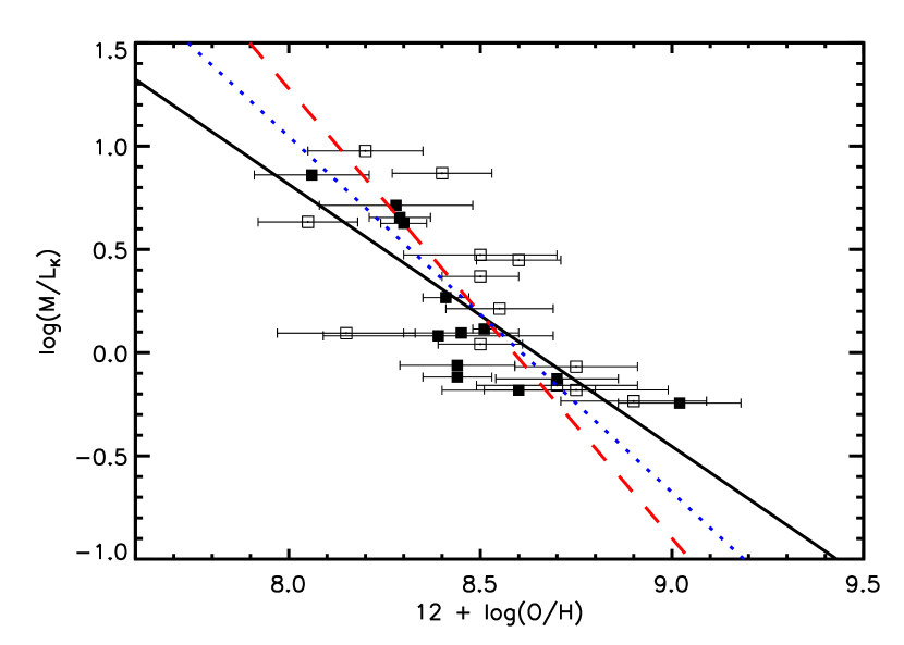
Figure 4.— M/L-metallicity relationship for H II regions (filled squares) and supergiant stars (open squares) in M33. The solid line represents the forward fit to the data, the dashed red line represents the fit to the inverse relationship, incorporating the metallicity uncertainties, and the blue dotted line is the linear bisector of the two (Equation 1)

.

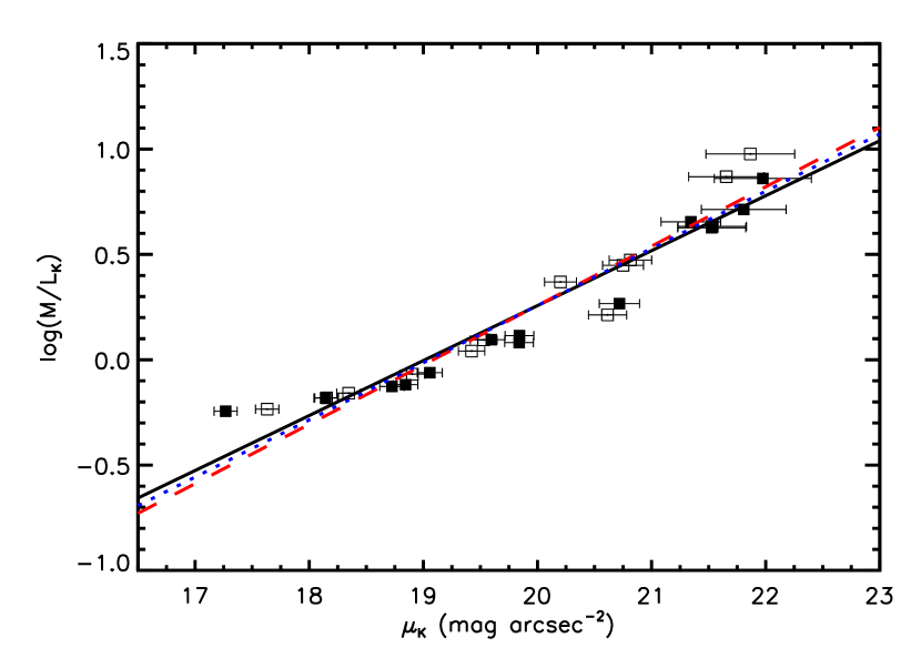
Figure 5.— M/L-surface brightness relationship for H II regions (filled squares) and supergiant stars (open squares) in M33. The solid line represents the fit to the data using M/L as the independent variable, the dashed red line represents the fit to the inverse relationship, incorporating the surface brightness uncertainties, and the blue dotted line is the linear bisector of the two (Equation 2)

.

Figure 6.— Surface brightness-metallicity relationship for H II regions (filled squares) and supergiant stars (open squares) in M33. The solid line represents the fit to the data given in Equation 3.

Before we proceed to fitting the data, a brief discussion of some of the subtleties involved is warranted. We are in the somewhat unusual situation of investigating relationships between three parameters, two of which have reasonably well-known and well-understood uncertainties (metallicity and surface brightness), and one of which does not (mass-to-light ratio). We do not know at this point whether one of these parameters physically causes the correlations with the others, so we should not assign the roles of independent and dependent variables in the fits. The most appropriate way of applying the standard technique of linear least squares fitting is therefore not clear. As discussed by Isobe et al. (1990) and Akritas & Bershady (1996), there are a number of fitting methods that can be used for linear regression problems. Because the relationships that we are investigating may have intrinsic scatter that is as large as or larger than the measurement uncertainties, we use the bivariate correlated errors and intrinsic scatter (BCES) method proposed by Akritas & Bershady (1996) as a generalization of ordinary least squares fitting. In order to avoid biasing the results by designating one variable as independent and one as dependent, for each pair of variables we run the BCES regression of $Y$ on $X$ as well as the BCES regression of $X$ on $Y$, and then take the linear bisector of the two as the best estimate of the true relationship.

3.1. Two-Parameter Correlations

We begin our analysis by considering the two-parameter correlations between M/L and metallicity, M/L and surface brightness, and metallicity and surface brightness. Following PB02, we fit the mass-to-light ratios at the position of each metallicity measurement as a function of the metallicities. Using a BCES fit with M/L as the dependent variable, we find the following relationship: $log{(M/L_{K})}=10.97\pm 1.73-(1.27\pm 0.20)[12+log(O/H)]$. Because the metallicities have known uncertainties, while the mass-to-light ratios do not, it might make more sense to carry out the inverse fit with metallicity as the dependent variable, which yields $12+log(O/H)=8.59\pm 0.04-(0.46\pm 0.08)log(M/L_{K})$. Converting this equation back into the form of the first equation, we find $log{(M/L_{K})}=18.69\pm 3.17-(2.18\pm 0.37)[12+log(O/H)]$, which differs from the forward fit at the $\sim 3$ $\sigma$ level in both coefficients. The reduced $\chi^{2}$ for this fit is 1.35. The forward and inverse fit results give a sense of the range of fits that are compatible with the data. Although there is a clear correlation between metallicity and mass-to-light ratio, the large scatter makes it difficult to define a precise relationship. Because the inverse fit incorporates additional information (the metallicity uncertainties), it is probably a more reliable estimate of the true correlation. The linear bisector (the average of the first and third equations) of the metallicity-M/L relationship is

$$log{(M/L_{K})}=14.83\pm 1.80-(1.72\pm 0.21)[12+log(O/H)].$$ (1)

The forward and inverse fits, along with the linear bisector, are plotted in Figure 4.

If we relax our assumption that the stellar disk of M33 is maximal and construct mass models with lower stellar mass-to-light ratios, we find only modest changes in the derived relationship. Even for the limiting case of a minimal disk (in which the stars do not contribute any mass to the galaxy), the fit parameters change by at most $\sim 1.95~{}\sigma$, in the direction of increasing zero point and decreasing (more negative) slope.

We then carry out the same process with the surface brightnesses. For the unweighted fit with M/L as the dependent variable, we find $log{(M/L_{K})}=-4.96\pm 0.34+(0.26\pm 0.02)\mu_{K}$. The inverse fit (including surface brightness uncertainties), gives $\mu_{K}=19.09\pm 0.10+(3.55\pm 0.23)log{(M/L_{K})}$ and when we rearrange this equation to write it in terms of M/L, we get $log{(M/L_{K})}=-5.38\pm 0.34+(0.28\pm 0.02)\mu_{K}$, this time in reasonably good agreement with the forward relationship. The formal reduced $\chi^{2}$ value for this fit is quite high (9.3) because of the small errors on the surface photometry near the center of the galaxy, indicating that the observed scatter is intrinsic to the relationship. Nevertheless, it is clear that the fitted lines are a good description of the data (see Figure 5). The linear bisector of the surface brightness-M/L correlation is

$$log{(M/L_{K})}=-5.17\pm 0.24+(0.27\pm 0.01)\mu_{K}.$$ (2)

For the M/L-surface brightness relationship, making the stellar disk less massive does have a statistically significant effect on the derived parameters. The linear bisector correlation for a submaximal ($V_{disk}/V_{tot}=0.6$) disk with $\mbox{$M_{*}/L_{K}$}=0.27\mbox{$M_{\odot}/L_{\odot K}$}$ is $log{(M/L_{K})}=-5.76+0.30\mu_{K}$, and for a minimal stellar disk the correlation is $log{(M/L_{K})}=-6.50+0.34\mu_{K}$.

Finally, for the metallicity-surface brightness relation, we obtain a best fit (taking uncertainties in both parameters into account) of

$$12+log(O/H)=10.99\pm 0.40-(0.13\pm 0.02)\mu_{K},$$ (3)

with a reduced $\chi^{2}$ value of 1.02 (see Figure 6). Note that in this case, since the observed scatter is consistent with being entirely attributable to the observational uncertainties, we do not need to use the BCES technique. We instead employ the method of Press et al. (1992) for linear fitting with errors in both coordinates. The inverse fit gives identical results for this relationship (which is not surprising, since the variables are treated completely symmetrically). This result is in excellent agreement with the $I$-band relationship derived by Ryder (1995) from measurements of 97 H II regions in six galaxies,

$$12+log(O/H)=10.91\pm 0.90-(0.095\pm 0.034)\mu_{I}.$$ (4)

3.2. The Fundamental Line

Having established the various two-parameter correlations between the data points, we now consider the best-fitting plane for all three parameters simultaneously. Using an unweighted ordinary least squares fit, we find that the fundamental line can be expressed as

$$log{(M/L_{K})} = -6.62\pm 1.42$$

$$+(0.15\pm 0.16)[12+log(O/H)]$$

$$+(0.28\pm 0.03)\mu_{K}.$$

The local fundamental line for M33 is plotted in Figure 7. The effect of increasing the assumed distance for M33 from 800 kpc to 900 kpc (see §2.1) is to slightly increase the constant offset in Equation 3.2 to $-6.47$. The metallicity coefficient is unchanged, and the surface brightness coefficient decreases to 0.27; all three terms change by much less than $1~{}\sigma$. Adjusting the mass model to allow for a lower mass stellar disk also does not significantly change the fundamental line. Even for a minimal stellar disk the constant term and the metallicity coefficient change by less than their uncertainties, and the surface brightness coefficient increases by $1.7~{}\sigma$. The derived fundamental line therefore appears to be robust against plausible systematic uncertainties in our assumptions. In Figure 8 we display edge-on and end-on views of the fundamental line in three dimensions, proving that the relationship is indeed a line and not a plane.

Figure 7.— The local fundamental line within M33. The filled squares represent H II regions and the open squares represent supergiants. The solid line shows the fit to the data given in Equation 3.2.

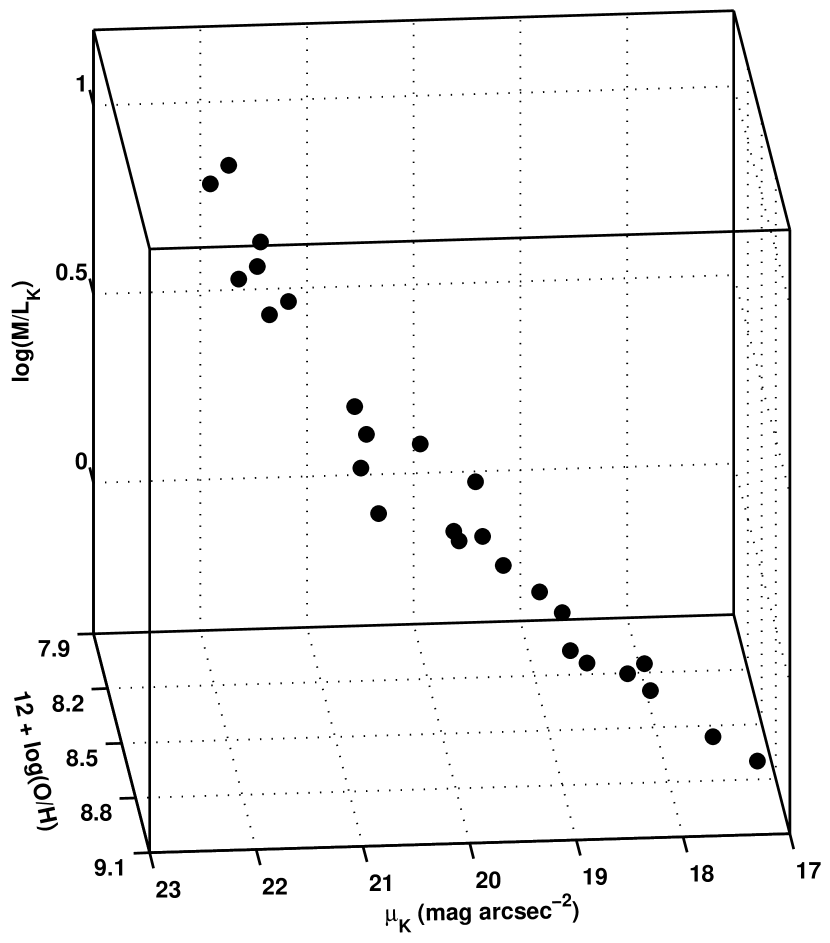
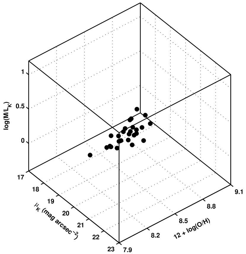
Figure 8.— Edge-on (left) and end-on (right) views of the fundamental line in the three-dimensional space (metallicity, surface brightness, log(M/L)). The narrowness of the fundamental line when observed end-on demonstrates that the points are indeed distributed in a line rather than a plane.

In contrast with the dwarf galaxy data, we find a very weak metallicity dependence for the fundamental line in M33. The metallicity dependence is also in the opposite sense of what we found when considering the two-parameter M/L-metallicity relationship. This may be partially caused by the small range of metallicities included in our sample ($\sim 1$ order of magnitude) and the relatively large uncertainties on those metallicities, but could also indicate a real difference between M33 and the Local Group dwarfs. In support of the former interpretation, it is worth noting that the M/L-metallicity correlation is the weakest of the three relationships studied in §3.1. Measurements of a large sample of metallicities including the innermost and outermost regions of M33 may be able to determine whether the metallicity dependence of the disk galaxy and dwarf galaxy fundamental lines actually differ.

3.2.1 The Curvature of the Fundamental Line

Despite the name that we have chosen for the fundamental line, inspection of Figure 7 suggests that rather than being truly linear, the fundamental line is actually slightly curved. At both the low M/L and high M/L ends of the line the data are curving upwards, towards larger mass-to-light ratios than the linear relation would predict. These deviations from linearity can be naturally understood by considering what the local values of M/L are physically describing. Near the center of the galaxy (at low M/L), the baryons contribute substantially to the total mass, increasing the mass-to-light ratio. If we used only the dark matter halo to calculate masses, then this end of the line would be more nearly straight (as we show explicitly in §4.2). The other end of the fundamental line also curves upward because there is almost no light being added at large radii, making the mass-to-light ratio increase more rapidly. Consistent with these explanations, we note that similar curvature is evident in the M/L-metallicity and M/L-surface brightness correlations, but not in the metallicity-surface brightness relationship, indicating that the origin of the curvature is in the mass-to-light ratio. Because of the limited extent of the available data, it is more useful to use the linear description of the fundamental line that we have derived rather than a quadratic one. However, future studies that employ larger data sets may be able to examine the curvature of the relationship in more detail.

4. DISCUSSION

In the previous section, we showed that not only are mass-to-light ratio, metallicity, and surface brightness all correlated with each other in M33, but also that a local fundamental line, which holds at every measured point within the disk of the galaxy, exists as well. We now examine this relationship in comparison to the dwarf galaxy fundamental line and consider its implications.

4.1. Comparison with the Fundamental Line of Dwarf Galaxies

Since the motivation for this work was the discovery of the fundamental line of dwarf galaxies, we would like to compare the relationships that we have found within M33 with the analogous relationships among dwarfs. Using linear least squares fits to the forward relationships, PB02 derived the following three correlations for the integrated properties of Local Group dwarfs:

$$log{(M/L_{V})}=-0.4-[Fe/H],$$ (6)

$$log{(M/L_{V})}=-5.35+0.27\mu_{V},$$ (7)

and

$$log{(M/L_{V})}=-2.86-0.56[Fe/H]+0.13\mu_{V}.$$ (8)

If we fit the same data using the BCES method, as we did for M33 in §3.1, we find that the coefficients differ at the $\sim 1-2$ $\sigma$ level:

$$log{(M/L_{V})}=-0.68\pm 0.13-(1.13\pm 0.09)[Fe/H]$$ (9)

and

$$log{(M/L_{V})}=-6.23\pm 0.53+(0.31\pm 0.02)\mu_{V}$$ (10)

In order to compare these fits properly with our results, we must derive conversions between the [Fe/H] and [12 + log(O/H)] abundance scales and $V$- and $K$-band mass-to-light ratios and surface brightnesses. A subset of the Local Group dwarf galaxies discussed by Mateo (1998) have both stellar [Fe/H] measurements and H II region oxygen abundances, from which we obtain

$$12+log(O/H)=9.5\pm 0.5+(1.1\pm 0.4)[Fe/H],$$ (11)

or alternatively,

$$[Fe/H]=-8.5\pm 2.6+(0.9\pm 0.3)[12+log(O/H)].$$ (12)

The abundance range spanned by the Local Group dwarf galaxies encompasses the abundance range of our data in M33 (see Figure 9).

Figure 9.— Comparison of the M/L-metallicity (left panel) and M/L-surface brightness (right panel) relationships within M33 and among the Local Group dwarfs. The M33 data are plotted as filled squares, and the dwarf galaxy points are plotted as open circles. The solid lines show the linear bisector fits to the M/L-metallicity and M/L-surface brightness relationships from Figures 4 and 5. The dashed (submaximal disk with $\mbox{$M_{*}/L_{K}$}=0.27$ $M_{\odot}/L_{\odot K}$) and dotted (minimal disk with $\mbox{$M_{*}/L_{K}$}=0$ $M_{\odot}/L_{\odot K}$) lines illustrate the effect of using different mass models for M33. Lowering the assumed stellar mass-to-light ratio does not improve the agreement between the M33 and dwarf galaxy data points.

$K$-band observations do not exist for many of the Local Group dwarfs, so the $V$- to $K$-band conversions must be derived specifically from the M33 data. M33 has integrated magnitudes of $m_{V}=5.37$ (de Vaucouleurs et al., 1991) and $m_{K}=2.73$ (both measurements are corrected for Galactic and internal extinction according to Schlegel, Finkbeiner, & Davis [1998] and Sakai et al. [2000], respectively), giving a $V-K_{s}$ color of 2.64. We can therefore estimate that

$$\log{M/L_{V}}=\log{M/L_{K}}+1.06$$ (13)

and

$$\mu_{V}=\mu_{K}+2.64.$$ (14)

Applying the conversion given in Equation 12 to the dwarf galaxy metallicities, we find that the dwarf galaxy M/L-metallicity relation (Equation 9) can be written

$$log{(M/L_{V})}=8.93\pm 3.04-(1.02\pm 0.35)[12+log(O/H)].$$ (15)

Converting the M33 relationships to $V$-band using Equations 13 and 14 gives M/L-metallicity and M/L-surface brightness relations of

$$log{(M/L_{V})}=15.89\pm 1.80-(1.72\pm 0.21)[12+log(O/H)]$$ (16)

and

$$log{(M/L_{V})}=-4.82\pm 0.24+(0.27\pm 0.01)\mu_{V}.$$ (17)

Comparing Equations 15 and 16, we see that both the slope and the zero point of the M/L-metallicity relationship are only marginally consistent (at the $\sim 2$ $\sigma$ level) between the Local Group dwarf galaxies and M33. The agreement between the global and local M/L-surface brightness relationships (Equations 10 and 17) is slightly worse, with a slope difference of $2$ $\sigma$ and a zero point offset of $2.7$ $\sigma$. However, as shown in Figures 9 and 10, for all three correlations the trends in the M33 data do appear roughly consistent with the trends among the Local Group dwarfs except for a zero-point offset. The local M/L in M33 is roughly a factor of 3 higher than the global M/L of a dwarf galaxy at the same surface brightness, and a factor of $5-10$ higher at the same metallicity. It is worth noting that using different mass models for M33 that place less mass in the stellar disk does not improve the agreement between the local and global relationships.

Figure 10.— Comparison of the surface brightness-metallicity relationships within M33 and among the Local Group dwarfs. The M33 data are plotted as filled squares, and the dwarf galaxy points are plotted as open circles.

Converting the M33 and dwarf galaxy fundamental lines to the common system of oxygen abundances and $V$-band magnitudes yields

$$log{(M/L_{V})}=1.90-0.50[12+\log{(O/H)}]+0.13\mu_{V}$$ (18)

for the dwarf galaxies, and

$$log{(M/L_{V})}=-6.30\pm 1.42+(0.15\pm 0.16)[12+\log{(O/H)}]+(0.28\pm 0.03)\mu_{V}$$ (19)

for M33. These relationships are clearly in rather poor agreement with each other. Nevertheless, a visual comparison again demonstrates that the variation of the mass-to-light ratio with metallicity and surface brightness is similar in M33 as it is for the dwarf galaxies (see Figure 11).

Figure 11.— Comparison of the fundamental line within M33 and the fundamental line of the Local Group dwarfs in the same units. The M33 data are plotted as filled squares, and the dwarf galaxy points are plotted as open circles.

The similarities in the slopes of all of these relationships indicate that there could be a connection between the local and global fundamental lines. However, M33 does not lie on the fundamental line of dwarfs, so the nature of this connection is not clear. Because structure forms hierarchically in the currently-favored Cold Dark Matter (CDM) cosmology, disk galaxies such as M33 were presumably constructed from the merging of many smaller galaxies. We suggest that simple simulations could be used to test whether a galaxy that is built up of smaller objects that obeyed the fundamental line of dwarf galaxies follows a local fundamental line like the one we observe in M33 at the present day. If not, what additional information is necessary to create the fundamental line?

4.2. The Origin of the Fundamental Line Correlations

4.2.1 The Metallicity-Surface Brightness Relation

The correlation between local surface brightness and metallicity in disk galaxies is well-known from previous work (e.g., Edmunds & Pagel, 1984; Ryder, 1995; Garnett et al., 1997; Bell & de Jong, 2000). This relationship is essentially a generic result of ordinary chemical evolution models. For example, if we treat M33 as a closed box, then the heavy element fraction $Z$ as a function of the gas fraction $\mu$ can be written as

$$Z(\mu)=-p\ln\mu,$$ (20)

where $p$ is the yield of heavy elements from each generation of star formation (Searle & Sargent, 1972). If we write out the expressions for $Z$ and $\mu$, then we have

$$\frac{M_{Z}}{M_{gas}}=-p\ln\left(\frac{M_{gas}}{M_{gas}+M_{*}}\right),$$ (21)

where $M_{Z}$ is the total mass of heavy elements and $M_{*}$ is the stellar mass. Now, we divide the mass terms on the right-hand side of the equation by a unit area to turn them into surface densities:

$$\frac{M_{Z}}{M_{gas}}=-p\ln\left(\frac{\Sigma_{gas}}{\Sigma_{gas}+\Sigma_{*}}\right).$$ (22)

After substituting the oxygen mass for the total heavy element mass, using $M_{O}=0.45M_{Z}$ (Garnett et al., 1997), and noting that $M_{gas}=1.33M_{H}$, we can rearrange Equation 22 to obtain the following for the metallicity-surface brightness relationship:

$$12+\log{(O/H)}=\log{\left[p\ln{\left(1+\frac{\Sigma_{*}}{\Sigma_{gas}}\right)}\right]+11.78}.$$ (23)

Solving this equation for the yield $p$ gives us

$$p=\frac{10^{12+\log{O/H}-11.78}}{\ln{\left(1+\Sigma_{*}/\Sigma_{gas}\right)}},$$ (24)

and, using the data from §3, we find that for $p=3.5\times 10^{-4}$ this model reproduces the observed metallicity-surface brightness correlation.

Alternatively, we can abandon the closed-box assumption and allow the infall of metal-poor gas onto M33. In this case, Clayton (1987) has shown that the heavy element fraction is

$$Z(\mu)=\frac{p}{2}\left[-\ln\mu+\ln\left(-\ln\mu+1\right)\right].$$ (25)

Proceeding through the same steps as above, we find that

$$p=\frac{10^{12+\log{O/H}-11.48}}{-\ln{\left(\frac{\Sigma_{gas}}{\Sigma_{gas}+\Sigma_{*}}\right)}+\ln{\left[1-\ln{\left(\frac{\Sigma_{gas}}{\Sigma_{gas}+\Sigma_{*}}\right)}\right]}}.$$ (26)

In this case also, for a yield of $p=4.5\times 10^{-4}$, we correctly recover the surface brightness-metallicity relationship in M33. It appears likely, then, that most plausible chemical enrichment scenarios will produce a strong correlation between metallicity and surface brightness. We therefore expect that all disk galaxies should display such a correlation. Galaxies that lie on the same correlation, as M33 and the sample studied by Ryder (1995) do, may have similar values for the heavy element yield.

4.2.2 The M/L-Surface Brightness Relation

Relationships between surface brightness and mass-to-light ratio have been recognized before on a global level (e.g., Zwaan et al., 1995; Zavala et al., 2003, although see Graham 2002), but the corresponding relationship within a single galaxy has received only minimal attention (Petrou, 1981). In order to understand the origin of the local M/L-surface brightness correlation that we found in §3.1, we consider a galaxy with an exponential stellar disk and a Navarro, Frenk, & White (1996, hereafter NFW) dark matter halo:

$$I(r) = I_{0}e^{-r/r_{d}}$$ (27)

$$\rho(r) = \frac{\delta_{c}\rho_{c}}{\frac{r}{r_{s}}\left(1+\frac{r}{r_{s}}\right)^{2}}.$$ (28)

Integrating the surface brightness profile over the circular disk area and the density profile over a spherical volume give the integrated luminosity and mass profiles of the galaxy, respectively:

$$L(r) = 2\pi I_{0}r_{d}^{2}\left[1-e^{-r/r_{d}}\left(1+\frac{r}{r_{d}}\right)\right]$$ (29)

$$M(r) = 4\pi\delta_{c}\rho_{c}r_{s}^{3}\left[\ln{\left(1+\frac{r}{r_{s}}\right)}-\frac{\frac{r}{r_{s}}}{1+\frac{r}{r_{s}}}\right].$$ (30)

Dividing the galaxy into concentric rings of width $\Delta r$, calculating the incremental mass ($\Delta M=M(r+\Delta r)-M(r)$) and light ($\Delta L=L(r+\Delta r)-L(r)$) in each ring using Equations 29 and 28, and then taking the ratio of the two yields

$$\frac{\Delta M}{\Delta L}=\frac{2\delta_{c}\rho_{c}r_{s}^{3}}{I_{0}r_{d}^{2}e^{-r/r_{d}}}\frac{\ln{(1+\frac{r+\Delta r}{r_{s}})}-\ln{(1+\frac{r}{r_{s}})}+\frac{r}{r+r_{s}}-\frac{r+\Delta r}{r+\Delta r+r_{s}}}{1+\frac{r}{r_{d}}-e^{-\Delta r/r_{d}}\left(1+\frac{r+\Delta r}{r_{d}}\right)}$$ (31)

for the local mass-to-light ratio. While this expression may look formidable, in fact its logarithm scales linearly with surface brightness (and radius) as long as $r_{s}\gg r_{d}$ (which is always true for real galaxies). Using reasonable values for the disk of M33 from this work and the halo from Corbelli (2003) (NFW concentration $c=10$ and scale radius $r_{s}=15$ kpc), we plot the M/L-surface brightness relation according to Equation 31 in Figure 12. There is reasonable agreement between the modeled and observed relationships. If the model had included the baryonic contribution to the total mass, which is significant at small radii (high surface brightnesses), then the solid line would curve upward at $\mu_{K}\lesssim 19$, following the data. Using other density profiles for the dark matter halo, such as a power law (as we assumed in §2.3) or a pseudo-isothermal profile, does not change the essentially linear correlation between $\log{M/L}$ and surface brightness, although in both of those cases the relationship does bend slightly upwards at high surface brightnesses rather than remaining exactly linear. Thus, the M/L-surface brightness correlation appears to be a universal property of galaxy disks that simply reflects the exponential nature of the disk and the increasing dark matter fraction as a function of radius.

Figure 12.— Model M/L-surface brightness relationship for a galaxy with an NFW dark matter halo and an exponential disk. The solid line shows the log of Equation 31 plotted against surface brightness, using parameters for the dark matter halo and stellar disk that are appropriate for M33. The solid points show the observed data for M33, and the dashed line gives the M/L-surface brightness relationship that we derived from the data in Equation 2.

4.2.3 The M/L-Metallicity Relation

Although the metallicity-surface brightness and M/L-surface brightness relationships follow generically from the basic processes that occur in galaxies, what is not clear is whether the M/L-metallicity relationship likewise is fundamental to the nature of disk galaxies, or if it is merely a residual correlation resulting from the other two relationships. Since the M/L-metallicity relationship has the largest scatter of the three, one might be justified in suspecting the latter. However, as we discussed in §1, PB02 proposed a model that can reproduce the global M/L-metallicity relationship in dwarfs, and simulations confirm that this result is plausible (Tassis et al., 2003). Therefore, it may be the case that there is a real local M/L-metallicity relationship in disks, but the relationship is weakened by the relatively large uncertainties on existing metallicity measurements. Future metallicity studies should be able to shed light on this possibility.

4.3. Implications

Previous work suggested that feedback might be responsible for the fundamental line of dwarf galaxies. Dekel & Woo (2003) studied the scaling relations among stellar mass, surface brightness, characteristic velocity, and metallicity for both the Local Group dwarfs and low-luminosity galaxies in the Sloan Digital Sky Survey database. They argued that a simple recipe for supernova feedback could reproduce the dwarf galaxy fundamental line. Tassis et al. (2003) used cosmological hydrodynamic simulations to show that a similar feedback model produces a M/L-metallicity relationship for dwarf galaxies consistent with that found by PB02. It therefore seems plausible that the same type of model might be able to explain the local fundamental line within M33 (note that M33 does lie within the mass range for which the Dekel & Woo scaling relations apply, with a stellar mass of $4\times 10^{9}$ M_⊙, compared to the mass of $3\times 10^{10}$ M_⊙ where the relationships change form). However, our analysis in §4.2 indicates that at least two of the three correlations that comprise the local fundamental line can be derived without appealing to feedback. Furthermore, other numerical work shows that both the local and global fundamental lines can be produced in simulations that do not contain feedback (§4.4 of this paper and A. Kravtsov 2005, personal communication).

If the Dekel & Woo (2003) picture is correct, then only galaxies below the transition mass of $\sim 3\times 10^{10}$ M_⊙ in stars ($\sim 6\times 10^{11}$ M_⊙ in total mass) should exhibit a local fundamental line. For more massive systems, Dekel (2004) suggests that feedback from active galactic nuclei plays an important role in shaping the evolution of galaxies. A critical test of the supernova feedback model is therefore whether a fundamental line relationship holds for massive, early-type disk galaxies and massive ellipticals. This test could be carried out for nearby galaxies with photometry of large samples of red giant branch stars (to measure the mean metallicity as a function of radius) along with long-slit spectroscopy to obtain the velocity dispersion profile (and hence M/L).

A further implication of the local fundamental line is that if low surface brightness (LSB) disk galaxies follow the fundamental line, then they should have large mass-to-light ratios and low metallicities. Observations clearly indicate that LSB galaxies are metal-poor (e.g., de Naray et al., 2004), and there is also evidence for higher mass-to-light ratios than are found in normal galaxies (Zwaan et al., 1995; de Blok & McGaugh, 1996, although see Sprayberry et al. 1995)

Finally, the fundamental line of M33 can also be used to place constraints on CDM simulations of the formation of disk galaxies. Hydrodynamic simulations of galaxy disks are beginning to approach the actual properties of observed disks in terms of size, mass, and rotation velocity, although the formation of bulgeless disks such as M33 is rare (e.g., Abadi et al., 2003; Robertson et al., 2004; Governato et al., 2004). The results of this paper show that realistic simulations of disks must also obey the fundamental line; if they do not, then the star formation and/or feedback recipes they include must not be correct. Current simulations are already detailed enough to investigate mass-to-light ratios, surface brightnesses, and metallicities on small physical scales, so in the following subsection we carry out this test.

4.4. The Fundamental Line in Simulations

We analyzed the fundamental line properties of the $\Lambda$CDM disk galaxy simulation of Robertson et al. (2004), updated using the GADGET2 code (Springel, 2005). The simulation uses the Springel & Hernquist (2003) model for the multiphase ISM to explore the impact of ISM pressurization by supernova feedback on disk galaxy formation, and produces a disk galaxy with a mass of $2.16\times 10^{11}h^{-1}$ M_⊙ and an exponential surface brightness profile (see Robertson et al. 2004 for further details).

We extracted mass-to-light ratios, K-band surface brightnesses, and gas metallicities from the simulation as follows. We calculated the angular momentum of the disk from the gas in order to define a face-on disk plane. Our measurements were then made in the plane of the disk. The K-band luminosity of the stellar particles was determined from the Bruzual & Charlot (2003) population synthesis models. The metallicity and surface brightness were measured in azimuthally averaged annuli, so these quantities are not truly local values as our observations are. However, the simulated galaxy is fairly axisymmetric (apart from a weak bar feature), so we do not expect this difference to affect the results. The mass-to-light ratios were calculated by directly measuring the dynamical mass in spherical shells and comparing with the luminosity contained in annuli at the same radii, essentially the same method that we used for M33.

We plot the M/L-metallicity, M/L-surface brightness, metallicity-surface brightness, and fundamental line relationships for the simulated galaxy in Figure 13. All of the trends we found in the M33 data in §3 are matched by the simulation, although there are also clear offsets between some of the actual relationships and the simulated ones, most notably involving the metallicity. Remarkably, though, the fundamental line is reproduced very nearly correctly in the simulation.

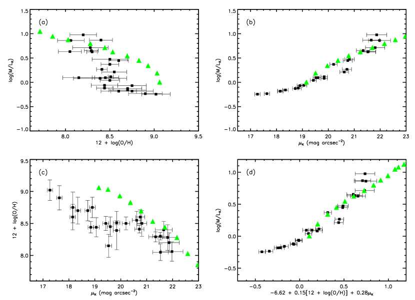
Figure 13.— Comparison of the scaling relationships in a simulated galaxy from Robertson et al. (2004) with the observed relationships in M33. (a) The M/L-metallicity relationship. (b) The M/L-surface brightness relationship. (c) The surface brightness-metallicity relationship. (d) The fundamental line. The black squares are the M33 data points, and the green triangles are the measurements of the simulated galaxy. All of the trends in the data are correctly reproduced in the simulation, although there is a significant zero-point offset in the simulation metallicities.

The gas metallicities seen in the simulation are too large by $\sim 0.6$ dex, which is not surprising because the simulation does not include a model for strong supernova-driven gas outflows. Also, simulated low-mass galaxies typically form too many stars given their total mass and gas content, thereby producing too many metals as well. The zero-point offsets in the left panels of Figure 13 are probably a result of these two effects. We interpret these results as an encouraging sign that the star formation and feedback models included in recent galaxy formation simulations require only modest adjustments in order to produce realistic stellar populations and chemical evolution.

In order to test whether the feedback in the simulation is what causes the fundamental line, we also ran a set of simple dissipational collapse simulations of disk galaxy formation. These simulations are comprised of 40,000 gas particles distributed in a fixed NFW dark matter halo with a virial mass of $M_{\mathrm{vir}}=2.16\times 10^{11}h^{-1}$ M_☉ (the same as the galaxy in the cosmological simulation from Robertson et al. [2004]). and a concentration of 15.24 (appropriate for the mass; Bullock et al. 2001). The initial galaxy has a gas fraction $f_{\mathrm{gas}}=0.1$ and is given a spin of $\lambda=0.1$. The simulations are then evolved for 2 Gyr. In each case, the gas cools and quickly settles into a disk (within $\sim 100$ Myr) and begins to form stars (see Springel & Hernquist 2003; Robertson et al. 2004). We model the ISM in these simulations using the Springel & Hernquist (2003) multiphase model, modified to include an effective equation of state parameter ($q_{\mathrm{EOS}}$) that linearly interpolates between an isothermal gas ($q_{\mathrm{EOS}}=0$) and an ISM strongly pressurized by supernova feedback ($q_{\mathrm{EOS}}=1$) as in the Robertson et al. (2004) simulation (see Springel & Hernquist 2003, Robertson et al. 2004, and Springel, Di Matteo, & Hernquist 2005 for further details). We simulate the dissipational collapse with various values of $q_{\mathrm{EOS}}$ between 0.01 and 1.0 to study the impact of the effects of supernova feedback on the fundamental line.

We find that when $q_{\mathrm{EOS}}$ is close to 0 (i.e., feedback is weak), all of the scaling relations have significant scatter (see Figure 14). In particular, for the M/L-metallicity and surface brightness-metallicity relationships, the scatter is nearly large enough to wipe out the correlations entirely. There are also noticeable zero-point offsets in each of the relationships, but since these simulations are intended to be simple models rather than realistic galaxies, we do not expect them to reproduce the observed scaling relations with high fidelity. Despite the scatter and the failure to produce accurate metallicities, a fundamental line is still apparent in these simulations. As $q_{\mathrm{EOS}}$ is increased towards 1, the relationships all tighten considerably, and the simulated points converge on the real data. This experiment suggests that feedback is responsible for the tightness of the fundamental line, but does not set the slope and zero point. It is worth noting that if we consider the M/L-metallicity, surface brightness-metallicity, and fundamental line relationships in terms of the mass-weighted gas+stellar metallicity instead of simply the ISM metallicity, good correlations (with scatter) are obtained even in the simulations with very weak feedback. In fact, with this metallicity prescription, the weak feedback correlations are generally closer to the observed correlations than the strong feedback results are (although again, they contain more scatter). Since the gas and stellar metallicities do not agree very well in these toy model simulations, it is not clear which metallicity definition offers the best comparison to our observations.

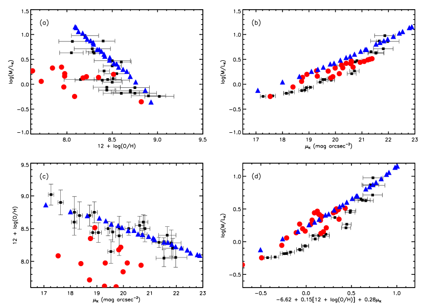
Figure 14.— Comparison of the scaling relationships in our dissipational collapse toy model simulations with the observed relationships in M33. (a) The M/L-metallicity relationship. (b) The M/L-surface brightness relationship. (c) The surface brightness-metallicity relationship. (d) The fundamental line. The black squares are the M33 data points, and the red circles and blue triangles are the measurements from the simulations in the cases of weak ($q_{\mathrm{EOS}}=0.01$) and strong ($q_{\mathrm{EOS}}=1$) feedback, respectively. The stronger feedback model clearly tightens all of the correlations and brings some of them closer to the observed relationships.

Although the results of these simulations appear promising in terms of matching the fundamental line, the substantial offsets seen in some of the component relationships suggest that we should be cautious in our interpretation. In a related example, while it is straightforward to generate numerical galaxy models that match the slope of the Tully-Fisher relation, simulations have not yet been able to simultaneously reproduce the slope, scatter, and zero point of the relation (e.g., Navarro & Steinmetz, 2000; Abadi et al., 2003; Dutton et al., 2006). By analogy, it is possible that the agreement we have found between the data and the simulations is fortuitous.

5. CONCLUSIONS

We have shown that there are strong correlations between dynamical mass-to-light ratio and metallicity, dynamical mass-to-light ratio and surface brightness, and metallicity and surface brightness that appear to hold locally, at every point within M33. The trends of these relationships are that low metallicity, low surface brightness regions have high M/L, and high metallicity, high surface brightness regions have low M/L. By analogy with the fundamental line of dwarf galaxies identified by PB02, we combine the three correlations into the fundamental line of disk galaxies (Figure 7), using local properties instead of global ones. The M33 data follow the same trends as the Local Group dwarf galaxies, but with zero-point offsets, such that at a given metallicity, the mass-to-light ratio in M33 is approximately a factor of $5-10$ higher than that of the dwarfs, and at a given surface brightness M33 has a mass-to-light ratio that is 3 times higher than the dwarf galaxies. These conclusions are largely independent of the particular mass model chosen for M33.

We demonstrated using analytical calculations that the metallicity-surface brightness relationship in galaxy disks is a generic prediction of ordinary chemical evolution models. Similarly, the M/L-surface brightness correlation can be derived straightforwardly under the assumptions of an exponential stellar disk and a dark matter halo that follows any of the proposed structures in the literature. It is not yet clear whether the M/L metallicity relationship shares a similar explanation or is merely a residual of the other two correlations. These results indicate that at least two of the three relationships that make up the local fundamental line originate from the basic properties of galaxy disks, and should therefore be universally applicable to other galaxies. Feedback, which was proposed by PB02, Dekel & Woo (2003), and Tassis et al. (2003) as the physical mechanism responsible for the fundamental line of dwarf galaxies, does not seem to play such an important role in the fundamental line of disk galaxies.

Finally, we compared the fundamental line relationships in M33 with their equivalents in a simulated disk galaxy from Robertson et al. (2004). We found good agreement in the slopes of each relationship, although the metallicity of the simulated galaxy is too high. Additional toy model simulations showed that feedback controls the tightness of the fundamental line, supporting the conclusion of our analytical models that feedback is not necessary to create the local fundamental line. Forcing simulated disks to match the fundamental line and its scatter will improve current numerical recipes for star formation and feedback.

References

- Abadi et al. (2003) Abadi, M. G., Navarro, J. F., Steinmetz, M., & Eke, V. R. 2003, ApJ, 591, 499
- Akritas & Bershady (1996) Akritas, M. G., & Bershady, M. A. 1996, ApJ, 470, 706
- Bell & de Jong (2000) Bell, E. F., & de Jong, R. S. 2000, MNRAS, 312, 497
- Bell & de Jong (2001) Bell, E. F., & de Jong, R. S. 2001, ApJ, 550, 212
- Blair & Kirshner (1985) Blair, W. P., & Kirshner, R. P. 1985, ApJ, 289, 582
- Blitz & Rosolowsky (2006) Blitz, L., & Rosolowsky, E. 2006, ApJ, in press (preprint: astro-ph/0605035)
- Block et al. (2004) Block, D. L., Freeman, K. C., Jarrett, T. H., Puerari, I., Worthey, G., Combes, F., & Groess, R. 2004, A&A, 425, L37
- Bruzual & Charlot (2003) Bruzual, G., & Charlot, S. 2003, MNRAS, 344, 1000
- Bullock et al. (2001) Bullock, J. S., Kolatt, T. S., Sigad, Y., Somerville, R. S., Kravtsov, A. V., Klypin, A. A., Primack, J. R., & Dekel, A. 2001, MNRAS, 321, 559
- Caldwell et al. (1998) Caldwell, N., Armandroff, T. E., Da Costa, G. S., & Seitzer, P. 1998, AJ, 115, 535
- Ciardullo et al. (2004) Ciardullo, R., Durrell, P. R., Laychak, M. B., Herrmann, K. A., Moody, K., Jacoby, G. H., & Feldmeier, J. J. 2004, ApJ, 614, 167
- Clayton (1987) Clayton, D. D. 1987, ApJ, 315, 451
- Corbelli (2003) Corbelli, E. 2003, MNRAS, 342, 199
- Corbelli & Salucci (2000) Corbelli, E., & Salucci, P. 2000, MNRAS, 311, 441
- Corbelli & Schneider (1997) Corbelli, E., & Schneider, S. E. 1997, ApJ, 479, 244
- de Blok & McGaugh (1996) de Blok, W. J. G., & McGaugh, S. S. 1996, ApJ, 469, L89
- Dekel (2004) Dekel, A. 2004, CfA Colloquium Lecture Series Talk (preprint: astro-ph/0401503)
- Dekel & Woo (2003) Dekel, A., & Woo, J. 2003, MNRAS, 344, 1131
- de Naray et al. (2004) de Naray, R. K., McGaugh, S. S., & de Blok, W. J. G. 2004, MNRAS, 355, 887
- de Vaucouleurs et al. (1991) de Vaucouleurs, G., de Vaucouleurs, A., Corwin, H. G., Buta, R. J., Paturel, G., & Fouque, P. 1991, Third Reference Catalog of Bright Galaxies (Berlin: Springer-Verlag)
- Dutton et al. (2006) Dutton, A. A., van den Bosch, F. C., Dekel, A., & Courteau, S. 2006, submitted to ApJ (preprint: astro-ph/0604553)
- Edmunds & Pagel (1984) Edmunds, M. G., & Pagel, B. E. J. 1984, MNRAS, 211, 507
- Engargiola et al. (2003) Engargiola, G., Plambeck, R. L., Rosolowsky, E., & Blitz, L. 2003, ApJS, 149, 343
- Garnett et al. (1997) Garnett, D. R., Shields, G. A., Skillman, E. D., Sagan, S. P., & Dufour, R. J. 1997, ApJ, 489, 63
- Graham (2002) Graham, A. W. 2002, MNRAS, 334, 721
- Governato et al. (2004) Governato, F., et al. 2004, ApJ, 607, 688
- Higdon et al. (2003) Higdon, S. J. U., Higdon, J. L., van der Hulst, J. M., & Stacey, G. J. 2003, ApJ, 592, 161
- Isobe et al. (1990) Isobe, T., Feigelson, E. D., Akritas, M. G., & Babu, G. J. 1990, ApJ, 364, 104
- Jarrett et al. (2003) Jarrett, T. H., Chester, T., Cutri, R., Schneider, S. E., & Huchra, J. P. 2003, AJ, 125, 525
- Kennicutt, Bresolin, & Garnett (2003) Kennicutt, R. C., Bresolin, F., & Garnett, D. R. 2003, ApJ, 591, 801
- Kim et al. (2002) Kim, M., Kim, E., Lee, M. G., Sarajedini, A., & Geisler, D. 2002, AJ, 123, 244
- Kwitter & Aller (1981) Kwitter, K. B., & Aller, L. H. 1981, MNRAS, 195, 939
- Lee et al. (2002) Lee, M. G., Kim, M., Sarajedini, A., Geisler, D., & Gieren, W. 2002, ApJ, 565, 959
- Magrini et al. (2003) Magrini, L., Perinotto, M., Corradi, R. L. M., & Mampaso, A. 2003, A&A, 400, 511
- Magrini et al. (2004) Magrini, L., Perinotto, M., Mampaso, A., & Corradi, R. L. M. 2004, A&A, 426, 779
- Mateo (1998) Mateo, M. L. 1998, ARA&A, 36, 435
- McConnachie et al. (2004) McConnachie, A. W., Irwin, M. J., Ferguson, A. M. N., Ibata, R. A., Lewis, G. F., & Tanvir, N. 2004, MNRAS, 350, 243
- Monteverde et al. (1997) Monteverde, M. I., Herrero, A., Lennon, D. J., & Kudritzki, R.-P. 1997, ApJ, 474, L107
- Navarro, Frenk, & White (1996) Navarro, J. F., Frenk, C. S., & White, S. D. M. 1996, ApJ, 462, 563
- Navarro & Steinmetz (2000) Navarro, J. F., & Steinmetz, M. 2000, ApJ, 538, 477
- Newton (1980) Newton, K. 1980, MNRAS, 190, 689
- Petrou (1981) Petrou, M. 1981, MNRAS, 196, 933
- Phillipps, Edmunds, & Davies (1990) Phillipps, S., Edmunds, M. G., & Davies, J. I. 1990, MNRAS, 244, 168
- Prada & Burkert (2002) Prada, F., & Burkert, A. 2002, ApJ, 564, L73 (PB02)
- Press et al. (1992) Press, W. H., Teukolsky, S. A., Vetterling, W. T., & Flannery, B. P. 1992, Numerical Recipes (Cambridge: University Press)
- Regan & Vogel (1994) Regan, M. W., & Vogel, S. N. 1994, ApJ, 434, 536
- Robertson et al. (2004) Robertson, B., Yoshida, N., Springel, V., & Hernquist, L. 2004, ApJ, 606, 32
- Ryder (1995) Ryder, S. D. 1995, ApJ, 444, 610
- Sakai et al. (2000) Sakai, S., et al. 2000, ApJ, 529, 698
- Schlegel, Finkbeiner, & Davis (1998) Schlegel, D. J., Finkbeiner, D. P., & Davis, M. 1998, ApJ, 500, 525
- Searle & Sargent (1972) Searle, L., & Sargent, W. L. W. 1972, ApJ, 173, 25
- Smith (1975) Smith, H. E. 1975, ApJ, 199, 591
- Sprayberry et al. (1995) Sprayberry, D., Bernstein, G. M., Impey, C. D., & Bothun, G. D. 1995, ApJ, 438, 72
- Springel (2005) Springel, V. 2005, submitted to MNRAS (preprint: astro-ph/0505010)
- Springel, Di Matteo, & Hernquist (2005) Springel, V., Di Matteo, T., & Hernquist, L. 2005, MNRAS, 361, 776
- Springel & Hernquist (2003) Springel, V., & Hernquist, L. 2003, MNRAS, 339, 289
- Stasińska et al. (2005) Stasińska, G., Vílchez, J. M., Pérez, E., Corradi, R. L. M., Mampaso, A., & Magrini, L. 2005, in “Planetary Nebulae as Astronomical Tools,”, AIP conference series, in press
- Tassis et al. (2003) Tassis, K., Abel, T., Bryan, G. L., & Norman, M. L. 2003, ApJ, 587, 13
- Teuben (1995) Teuben, P. J. 1995, in ASP Conf. Ser. 77: Astronomical Data Analysis Software and Systems IV, ed. R. Shaw, H. E. Payne, & J. J. E. Hayes (San Francisco: ASP), 398
- Urbaneja (2004) Urbaneja, M. A. 2004, Ph.D. Thesis, University of La Laguna
- Urbaneja et al. (2005) Urbaneja, M. A., Herrero, A., Kudritzki, R.-P., Najarro, F., Smartt, S. J., Puls, J., Lennon, D. J., & Corral, L. J. 2005, ApJ, in press
- Vílchez et al. (1988) Vílchez, J. M., Pagel, B. E. J., Díaz, A. I., Terlevich, E., & Edmunds, M. G. 1988, MNRAS, 235, 633
- Zavala et al. (2003) Zavala, J., Avila-Reese, V., Hernández-Toledo, H., & Firmani, C. 2003, A&A, 412, 633
- Zwaan et al. (1995) Zwaan, M. A., van der Hulst, J. M., de Blok, W. J. G., & McGaugh, S. S. 1995, MNRAS, 273, L35