Suppressing the contribution of intrinsic galaxy alignments to the shear two-point correlation function

Cosmological weak lensing gives rise to correlations in the ellipticities of faint galaxies. This cosmic shear signal depends upon the matter power spectrum, thus providing a means to constrain cosmological parameters. It has recently been proposed that intrinsic alignments arising at the epoch of galaxy formation can also contribute significantly to the observed correlations, the amplitude increasing with decreasing survey depth. Here we consider the two-point shear correlation function, and demonstrate that photometric redshift information can be used to suppress the intrinsic signal; at the same time Poisson noise is increased, due to a decrease in the effective number of galaxy pairs. The choice to apply such a redshift-depending weighting will depend on the characteristics of the survey in question. In surveys with $\left\langle z\right\rangle\sim 1$, although the lensing signal dominates, the measurement error bars may soon become smaller than the intrinsic alignment signal; hence, in order not to be dominated by systematics, redshift information in cosmic shear statistics will become a necessity. We discuss various aspects of this.

1 Introduction

The distortion of distant galaxies by the tidal gravitational field of intervening matter inhomogeneities has become known as “cosmic shear”. Since this lensing signal depends upon the matter power spectrum, it is an important cosmological tool, as was proposed in the early 1990s by Blandford et al. (1991), Miralda-Escudé (1991) and Kaiser (1992). This set the scene for further analytic and numerical work (eg. Kaiser 1998; Schneider et al. 1998; White & Hu 2000), taking into account the non-linear evolution of the power spectrum which results in increased power on small scales (Hamilton et al. 1991; Peacock & Dodds 1996).

During 2000, four teams announced the first observational detections of cosmic shear (Bacon et al. 2000; Kaiser et al. 2000; van Waerbeke et al. 2000; Wittman et al. 2000; Maoli et al. 2001), demonstrating the feasibility of its study. Various statistics are used to quantify cosmic shear, and to compare the observations with predictions for cosmological models. Here we focus on the shear correlation functions; other measures include the aperture mass statistic (Schneider et al. 1998) and shear variance (e.g. Kaiser 1992).

Besides its dependence on the large-scale structure in the Universe, the magnitude of the effect is also sensitive to the redshift distribution of the galaxies used in the analysis. So far, direct redshift estimates have not been obtained for the samples concerned. Typically the mean redshift has been estimated from surveys of similar depth, and a corresponding redshift probability distribution has been assumed (e.g. van Waerbeke et al. 2001; Hoekstra et al. 2002a). Motivated by the recent interest in obtaining photometric redshifts for cosmic shear surveys, we consider how to make use of redshift information, and its impact on the constraints permitted by the two-point statistic under consideration.

In weak lensing analyses, it is assumed that the background galaxies are randomly oriented so that their mean intrinsic ellipticity $\left\langle\epsilon^{\rm s}\right\rangle=0$ and any correlation in observed ellipticities arises from gravitational lensing. The magnitude of any intrinsic alignment of the background source population has recently been the subject of many numerical, analytic and observational studies (e.g. Croft & Metzler 2000; Heavens et al. 2000; Crittenden et al. 2001 (Cr01); Catelan et al. 2001; Mackey et al. 2002; Brown et al. 2002, Hui & Zhang 2002). Due to differences in the assumed origin of intrinsic alignments and the type of galaxies considered, the numerical and analytic estimates span a couple of orders of magnitude in amplitude. For example, the analytic model of Cr01 assumes that any intrinsic signal arises from correlations between the angular momenta of galaxies, whereas that of Catelan et al. (2001) relies on tidal shear correlations. Nonetheless, all studies conclude that intrinsic alignments are more important for shallower surveys (becoming comparable to the lensing signal for a mean survey redshift ${\left\langle z\right\rangle}\sim 0.5$) and that the correlation falls off quite rapidly with source separation.

The structure of this paper is as follows. In the next section we outline the relationships between the matter power spectrum and the lensing correlation functions. The dependence on the redshift distribution and on cosmology is highlighted. Correlation functions are derived from observational data, and in ${\rm Sect.\,3}$ we describe how practical estimators are used for this purpose. In ${\rm Sect.\,4}$ a toy model to account for intrinsic alignments is developed; the amplitude of the correlation is normalised to that of Cr01. The introduction of a weighting factor to minimise any contribution of intrinsic alignments to the shear correlation function is considered in ${\rm Sect.\,5}$. In ${\rm Sect.\,6}$ we present the results of applying such a weighting factor to surveys of different mean redshift. We finish in ${\rm Sect.\,7}$ with a discussion of the results and a future perspective of using redshift information in cosmic shear analysis.

For a review of cosmological weak lensing and the relevant aspects of cosmology, see Mellier (1999) and Bartelmann & Schneider (2001; hereafter BS01). In addition, the present status and outlook for cosmic shear studies is summarised by van Waerbeke et al. (2002).

2 Power spectra and lensing correlation functions

In this section, the relationships between the power spectra and observable lensing correlation functions are outlined; throughout, we adopt the notation of BS01.

The three-dimensional density fluctuation field $\delta({\hbox{$\bf r$}})$ at comoving position $\bf r$ is a homogeneous and isotropic random field, with a two-point correlation function given by

$$\left\langle\delta({\hbox{$\bf r$}})\delta({\hbox{$\bf r^{\prime}$}})\right\rangle\equiv C_{\delta\delta}\left(|{\hbox{$\bf r$}}-{\hbox{$\bf r^{\prime}$}}|\right)\;.$$ (1)

Such a field is described by its power spectrum $P_{\delta}(|{\hbox{$\bf k$}}|)$ ($\bf k$ being the comoving wave-vector), which is the Fourier transform of the two-point correlation function. In Fourier space one can write

$$\left\langle\hat{\delta}({\hbox{$\bf k$}})\hat{\delta}^{*}({\hbox{$\bf k$}}^{\prime})\right\rangle\equiv(2\pi)^{3}\delta_{\rm D}({\hbox{$\bf k$}}-{\hbox{$\bf k$}}^{\prime})P_{\delta}(|{\hbox{$\bf k$}}|)\;,$$ (2)

where $x^{*}$ denotes the complex conjugate of $x$, $\hat{x}$ denotes its Fourier transform, and $\delta_{\rm D}$ is the Dirac delta function.

The effective convergence $\bar{\kappa}_{\rm eff}({\hbox{$\bf\theta$}})$ depends upon the weighted integral of the density contrast along the line of sight

$$\bar{\kappa}_{\mathrm{eff}}(\@vec{\theta})=\frac{3H_{0}^{2}\Omega_{\rm m}}{2c^{2}}\,\int_{0}^{w_{\mathrm{H}}}\,{\rm d}w\,\bar{W}(w)\,f(w)\,\frac{\delta[f(w)\@vec{\theta},w]}{a(w)}\;,$$ (3)

where $H_{0}$ and $\Omega_{\rm m}$ are the values of the Hubble parameter and the density parameter at the present epoch, and $a(w)$ is the scale factor at comoving distance $w$, normalized such that $a(0)=1$ today. The horizon distance is denoted by $w_{\mathrm{H}}$, and $f(w)$ is the comoving angular diameter distance, so that the comoving separation is $f(w){\hbox{$\bf\theta$}}$. The function $f(w)$ depends on the spatial curvature, $K$:

$$f(w)=\left\{\begin{array}[]{ll}K^{-1/2}\sin(K^{1/2}w)&(K>0)\\ w&(K=0)\\ (-K)^{-1/2}\sinh[(-K)^{1/2}w]&(K<0)\\ \end{array}\right.\;;$$ (4)

later we assume that $K=0$ (i.e. $\Omega_{\rm m}\;+\;\Omega_{\Lambda}=1$). The function $\bar{W}(w)$ accounts for the sources being distributed in redshift, and consequent differences in lensing signal,

$$\bar{W}(w)\equiv\int_{w}^{w_{\mathrm{H}}}{\rm d}w^{\prime}\,p(w^{\prime})\,\frac{f(w^{\prime}-w)}{f(w^{\prime})}\leavevmode\nobreak\ \leavevmode\nobreak\ \leavevmode\nobreak\ \equiv\left\langle R(w,w^{\prime})\right\rangle\;,$$ (5)

where $p(w^{\prime})dw^{\prime}$ is the comoving distance probability distribution for the sources. The function $R(w,w^{\prime})=f(w^{\prime}-w)/f(w^{\prime})$ is the ratio of the angular diameter distance of a source at comoving distance $w^{\prime}$ seen from a distance $w$, to that seen from $w=0$.

The power spectrum $P_{\kappa}(\ell)$ of the effective convergence, or equivalently of the shear $P_{\gamma}(\ell)$ (see for example BS01), is related to that of the density fluctuations through a variant of Limber’s equation in Fourier space (Kaiser 1998)

$$P_{\kappa}(\ell)=\frac{9H_{0}^{4}\Omega_{\rm m}^{2}}{4c^{4}}\,\int_{0}^{w_{\mathrm{H}}}\,{\rm d}w\,\frac{\bar{W}^{2}(w)}{a^{2}(w)}\,P_{\delta}\left(\frac{\ell}{f(w)},w\right)\;,$$ (6)

where $\@vec{\ell}$ is the angular wave-vector, Fourier space conjugate to $\@vec{\theta}$.

We see now that $P_{\kappa}$ and $P_{\gamma}$ are intimately related to $\Omega_{\rm m}$, and to $P_{\delta}$ which in turn depends on $\Omega_{\Lambda}$, the shape parameter $\Gamma$ and on $\sigma_{8}$, the density fluctuations in spheres of radius $8h^{-1}{\rm Mpc}$. In addition, note the dependence upon the redshift distribution of the sources. Access to the cosmological parameters is provided through the (observable) shear correlation functions, which we now turn to.

The shear has two components and can conveniently be represented as the complex quantity $\gamma\equiv\gamma_{1}\,+\,{\rm i}\gamma_{2}$. Throughout, we assume the weak lensing limit so that $|\gamma|\ll 1$. Consider a pair of galaxies at position $\bf{\vartheta}$ and ${\hbox{$\bf{\vartheta}$}}\,+\,{\hbox{$\bf\theta$}}$, where the polar angle of their separation vector $\bf\theta$ is $\phi$. The tangential and cross-components of the shear for either of these galaxies are

$$\gamma_{\rm t}=-{\cal R}\hbox{e}\left[\gamma{\rm e}^{-2i\phi}\right];\leavevmode\nobreak\ \leavevmode\nobreak\ \leavevmode\nobreak\ \leavevmode\nobreak\ \gamma_{\times}=-{\cal I}\hbox{m}\left[\gamma{\rm e}^{-2i\phi}\right].$$ (7)

Using the notation of Schneider et al. (2002a), the shear correlation functions are defined as

$$\xi_{\pm}(\theta)=\left\langle\gamma_{\rm t}\gamma_{\rm t}\right\rangle\pm\left\langle\gamma_{\times}\gamma_{\times}\right\rangle(\theta)=\int_{0}^{\infty}{{\rm d}\ell\,\ell\over 2\pi}\,{\rm J}_{0,4}(\ell\theta)\;P_{\kappa}(\ell)\;,\\$$ (8)

where J_n are $n$-th order Bessel functions of the first kind. $P_{\kappa}(\ell)$ can be written in terms of the observable correlation functions:

$$P_{\kappa}(\ell)=2\pi\int_{0}^{\infty}{\rm d}\theta\,\theta\,\left[\xi_{\pm}(\theta){\rm J}_{0,4}(\ell\theta)\right]\;,$$ (9)

making use of the orthogonality of Bessel functions. From now on we focus on $\xi_{+}$, since this contains most cosmological information on the scales of interest.

Another quantity that is often determined in cosmological weak lensing studies is the shear variance inside a circle of radius $\theta_{\rm c}$, which is also related to the convergence power spectrum

$$\left\langle\left|\bar{\gamma}\right|^{2}\right\rangle(\theta_{\rm c})={1\over 2\pi}\int{\rm d}\ell\,\ell\,P_{\kappa}(\ell)\,{4{\rm J}_{1}^{2}(\ell\theta_{\rm c})\over\left(\ell\theta_{\rm c}\right)^{2}}\;.$$ (10)

This can also be determined directly by placing circular apertures onto the data field but is affected by any gaps; these may arise, for example, due to the need to mask regions containing bright stars and their diffraction spikes. However, the shear variance can also be obtained from $\xi_{+}$:

$$\left\langle\left|\bar{\gamma}\right|^{2}\right\rangle(\theta_{\rm c})=\int{{\rm d}{\vartheta}\,{\vartheta}\over\theta_{\rm c}^{2}}\,\xi_{+}({\vartheta})\,S_{+}\left({\vartheta}\over\theta_{\rm c}\right)\;,$$ (11)

where van Waerbeke (2000) showed that

$$S_{+}(x)=\left\{\begin{array}[]{ll}{1\over\pi}\left[4\cos^{-1}\left(x\over 2\right)-x\sqrt{4-x^{2}}\right]&(x\leq 2)\\ 0&(x>2)\\ \end{array}\right.\;.$$ (12)

2.1 Choice of cosmology, power spectrum and source redshift distribution

Unless otherwise stated, our fiducial cosmology is a $\Lambda$CDM model with $\Omega_{\rm m}=0.3$, $\Omega_{\Lambda}=0.7$ and $H_{0}=70\,{\rm km}\,{\rm s}^{-1}\,{\rm Mpc}^{-1}$.

A scale-invariant ($n=1$, Harrison-Zel’dovich) spectrum of primordial fluctuations is assumed. Predicting the shear correlation functions requires a model for the redshift evolution of the 3-D power spectrum. The fitting formula of Bardeen et al. (1986; BBKS) is used for the transfer function, and the Peacock and Dodds (1996) prescription for the evolution in the nonlinear regime. The power spectrum normalisation is parameterised with $\sigma_{8}=0.9$, and the shape parameter $\Gamma=0.21$.

As an aside, the differences in predicted shear correlation functions using the fitting formula of Eisenstein & Hu (1999) for the transfer function (rather than that of BBKS) were found to be minimal.

The normalised source redshift distribution is parameterised using the form suggested by Smail et al. (1995):

$$p(z){\rm d}z=\frac{\beta}{z_{0}\Gamma_{\gamma}\left(3/\beta\right)}\left(\frac{z}{z_{0}}\right)^{2}{\rm exp}\left[-\left(\frac{z}{z_{0}}\right)^{\beta}\right]\,{\rm d}z\;,$$ (13)

where $\Gamma_{\gamma}(x)$ is the gamma function. We set $\beta=1.5$ so that $\left\langle z\right\rangle\approx 1.5\,z_{0}$. The value of $z_{0}$ is adjusted to give different redshift distributions, which would in practice be obtained from surveys with different limiting magnitudes. For example, Fig. 1 shows $p(z)$ for $\left\langle z\right\rangle=0.5$ and $\left\langle z\right\rangle=1.0$, roughly corresponding to limiting magnitudes of $I\sim 22$ and $\sim 25$ respectively.

Figure 1: Normalised source redshift distributions, $p(z)$, for $\left\langle z\right\rangle=0.5$ (solid curve) and $\left\langle z\right\rangle=1.0$ (dashed curve) using the parameterisation of Smail et al. (1995).

2.2 Some dependencies of $\xi_{+}$

In this subsection we note some dependencies of $\xi_{+}$ on cosmological parameters, and on the redshift distribution of the sources from which it is measured.

To illustrate the dependency of $\xi_{+}$ on source redshift distribution, Fig. 2 shows $\xi_{+}$ for three values of $z_{0}$, corresponding to $\left\langle z\right\rangle=0.8$, 1.0 and 1.2. As expected, the amplitude of $\xi_{+}$ is higher for deeper surveys. Fig. 2 also highlights a couple of degeneracies: $\xi_{+}$ for $\left\langle z\right\rangle=1.0$, now with $\Omega_{\rm m}=0.38$ is shown. Note the difficulty in distinguishing this curve from that of the fiducial cosmology with a higher mean redshift, $\left\langle z\right\rangle=1.2$. The well-known degeneracy between $\Omega_{\rm m}$ and $\sigma_{8}$ is also demonstrated: we show that for $\left\langle z\right\rangle=1.0$, taking for instance $\Omega_{\rm m}=0.4$ and $\sigma_{8}=0.78$ results in a curve which would be difficult to distinguish from that of the fiducial cosmology in practice.

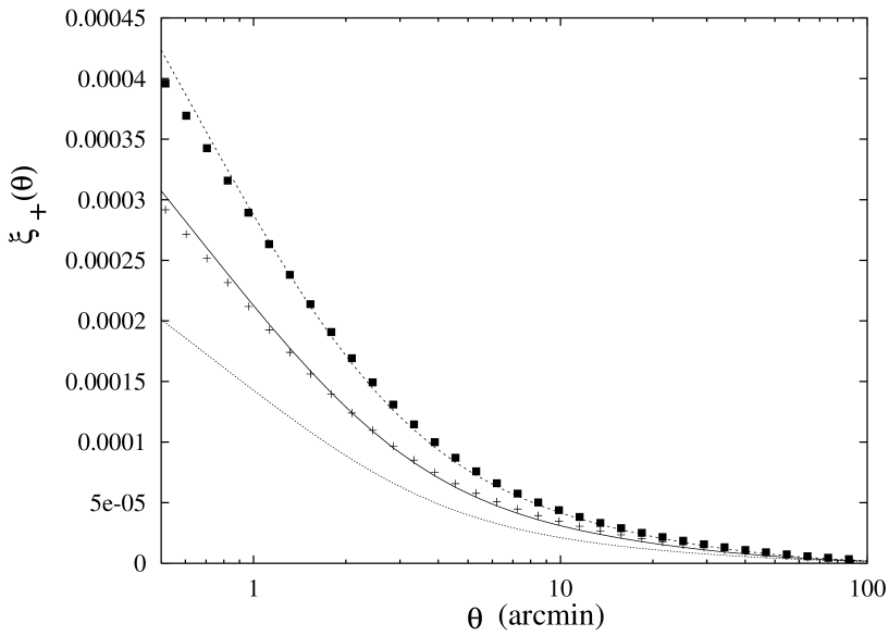
Figure 2: Dependence of $\xi_{+}$ on angular scale $\theta$ for $\left\langle z\right\rangle=0.8$ (dotted curve), $\left\langle z\right\rangle=1.0$ (solid curve) and $\left\langle z\right\rangle=1.2$ (short dashed curve). The cosmology for these curves is as described in the text, with $\Omega_{\rm m}=0.3$. The solid boxes correspond to $\left\langle z\right\rangle=1.0$, now with $\Omega_{\rm m}=0.38$. The crosses represent $\left\langle z\right\rangle=1.0$, $\Omega_{\rm m}=0.4$ and $\sigma_{8}=0.78$.

3 Estimators

Let us now consider how estimates of the correlation functions can be obtained in practice using the distorted images of galaxies. We begin by considering the case where the only mechanism giving rise to correlations in galaxy ellipticities is gravitational lensing.

In the limit of weak lensing, the complex ellipticity of a galaxy ${\epsilon}_{i}$ at position $\@vec{\theta}_{i}$ is related to its intrinsic ellipticity ${\epsilon^{\rm s}}\!\!_{i}$ and to the gravitational shear $\gamma(\@vec{\theta}_{i})$ through

$${\epsilon}_{i}={\epsilon^{\rm s}}\!\!_{i}+\gamma(\@vec{\theta}_{i})\;.$$ (14)

We use the definition of ellipticity from Bonnet & Mellier (1995) where for elliptical isophotes with axis ratio $b/a\leq 1$, $|{\epsilon}|=(1-b/a)(1+b/a)^{-1}$. Further, under this definition $\left\langle{\epsilon}\right\rangle\approx\gamma$ if the unlensed source population is randomly oriented. For simplicity we will use the notation $\gamma_{i}\equiv\gamma(\@vec{\theta}_{i})$. Using (14) it follows that the expectation value

$$\left\langle{\epsilon}_{i}{\epsilon}_{j}^{*}\right\rangle\equiv\left\langle\left({\epsilon^{\rm s}}\!\!_{i}+\gamma_{i}\right)\left({{\epsilon^{\rm s}}^{*}}\!\!\!\!_{j}+\gamma^{*}_{j}\right)\right\rangle\equiv\left\langle\gamma_{i}\gamma_{j}^{*}\right\rangle+\left\langle{\epsilon^{\rm s}}\!\!_{i}{{\epsilon^{\rm s}}^{*}}\!\!\!\!_{j}\right\rangle\;,$$ (15)

and in the absence of intrinsic correlations the final term vanishes. In this case, any correlation between observed galaxy ellipticities results from weak lensing.

As discussed in Schneider et al. (2002b), the correlation function can be estimated in bins of width $\Delta{\vartheta}$, centred on ${\vartheta}$, and a weight function can be defined such that $\Delta_{{\vartheta}}(\phi)=1$ for ${\vartheta}-\Delta{\vartheta}/2<\phi\leq{\vartheta}+\Delta{\vartheta}/2$ and is zero otherwise. An estimator for the correlation function $\xi_{+}({\vartheta})$ is given by

$$\hat{\xi}_{+}({\vartheta})=\frac{\sum_{ij}{\mathcal{W}}_{i}{\mathcal{W}}_{j}\Delta_{{\vartheta}}\left(|\@vec{\theta}_{i}-\@vec{\theta}_{j}|\right)\left({\epsilon}_{i}{\epsilon}_{j}^{*}\right)}{N_{\rm p}({\vartheta})}\;,\leavevmode\nobreak\ \leavevmode\nobreak\ \leavevmode\nobreak\ N_{\rm p}({\vartheta})=\sum_{ij}{\mathcal{W}}_{i}{\mathcal{W}}_{j}\Delta_{{\vartheta}}\left(|\@vec{\theta}_{i}-\@vec{\theta}_{j}|\right)\;,$$ (16)

where ${\mathcal{W}}_{i}$ and ${\mathcal{W}}_{j}$ are weights (depending on the reliability of the ellipticity measurement, for example) and $N_{\rm p}({\vartheta})$ is the effective number of pairs in that bin. In the absence of intrinsic correlations, since $\left\langle{\epsilon}_{i}{\epsilon}^{*}_{j}\right\rangle\equiv\xi_{+}(|{\hbox{$\bf\theta$}}_{i}-{\hbox{$\bf\theta$}}_{j}|)$, it follows that $\hat{\xi}_{+}({\vartheta})$ is an unbiased estimator of the shear correlation function of the lensing signal $\xi_{+}({\vartheta})$.

However, the existence of intrinsic alignments would imply that $\left\langle{\epsilon^{\rm s}}\!\!_{i}{{\epsilon^{\rm s}}^{*}}\!\!\!\!_{j}\right\rangle\neq 0$. The estimator $\hat{\xi}_{+}({\vartheta})$ is no longer an unbiased estimator of $\xi_{+}({\vartheta})$: rather it includes a contribution from correlated intrinsic (source) ellipticities, for which the two-point correlation function will be denoted by $\xi_{+}^{\rm int}({\vartheta})$. In order to minimise the impact of intrinsic correlations on the interpretation of the weak lensing signal, we need an estimate of the amplitude of $\xi_{+}^{\rm int}({\vartheta})$, and a scheme to give less weight to galaxy pairs where the intrinsic correlation is likely to be high.

4 Intrinsic alignments

Correlations between the intrinsic ellipticities of neighbouring galaxies are expected to arise during their formation, due to similarities in the tidal gravitational field in which they form. As noted in the introduction, a number of numerical and analytical studies have sought to quantify the amplitude of this correlation as a function of angular separation and redshift. For our purposes, we need a toy model to roughly predict the amplitude of intrinsic correlations expected. Since there is disagreement on the dominant mechanism responsible for intrinsic alignments, and on its subsequent enhancement or “washing out”, use of a detailed model is not warranted here.

Let us consider a close pair of galaxies with comoving distances $w_{i}\approx w_{j}\approx w$ and angular separation $\theta$. Their comoving separation $r$ is given by

$$r^{2}=(\Delta w)^{2}+f^{2}(w)(\theta)^{2}\;,$$ (17)

where $\Delta w\approx w_{i}-w_{j}$.

Denoting the (3-D) two-point density correlation function by $\xi_{\delta}(r)$, one might expect that the two-point correlations in intrinsic ellipticity $\propto\xi_{\delta}^{2}(r)$. Indeed, this dependence corresponds to the asymptotic behaviour at large separations derived by Cr01, whose normalisation we later adopt. The two-point density correlation function is the Fourier transform of the power spectrum, so the power spectrum used to predict the lensing correlation functions described in Sect. 2 could be used. However, since Cr01 focus on a $\xi_{\delta}(r)\propto 1/r$ behaviour, and because of its analytic simplicity, we also use this form.

Next, this 3-D intrinsic correlation function has to be projected into an angular intrinsic ellipticity correlation function, integrating over the distance distribution of galaxies and taking into account the (observed) galaxy two-point correlation function $\xi_{\rm gg}(r)$. Note that we do not consider the individual tangential and cross components of the correlation functions of the intrinsic ellipticities. Rather, we consider the sum of these quantities, which corresponds to $\xi_{+}$ in the notation of Schneider et al. (2002a; note that the notation of Cr01 differs here). We obtain

$$\xi_{+}^{\rm int}(\theta)\propto\frac{\int{\rm d}w_{1}\,p(w_{1})\int{{\rm d}w_{2}\,p(w_{2})[1+\xi_{\rm gg}(r)]\left[\xi_{\delta}(r)\right]^{2}}}{\int{\rm d}w_{1}\,p(w_{1})\int{{{\rm d}w_{2}\,p(w_{2})[1+\xi_{\rm gg}(r)]}}}\;,$$ (18)

where $p(w){\rm d}w$ is the galaxy distance distribution, which we take to be of the form given in Sect. 2.

Given that the scale over which intrinsic alignments operate is much smaller than the distances to the galaxies, the integral above can be recast as

$$\xi_{+}^{\rm int}(\theta)\propto\frac{\int{{\rm d}w\;p^{2}(w)\;\int{{\rm d}(\Delta w)\;[1+\xi_{\rm gg}(r)]\;\left[\xi_{\delta}(r)\right]^{2}}}}{1\;+\;\int{{\rm d}w\;p^{2}(w)\;\int{{\rm d}(\Delta w)\;\left[\xi_{\rm gg}(r)\right]}}}\;.$$ (19)

The two-point galaxy correlation function is taken to be $\xi_{\rm gg}(r)=(r/4.3\;h^{-1}{\rm Mpc})^{-1.8}$, constant in comoving separation. Evolution is ignored for both the galaxy and density correlation functions, in view of the weak evolution that is seen in galaxy samples out to $z\sim 3$ (e.g. Porciani & Giavalisco 2002). The normalisation of $\xi_{+}^{\rm int}(\theta)$ is set at an angular scale of $10\arcmin$ and for $\left\langle z\right\rangle=1$, using the value obtained by Cr01; Mackey et al. (2002) point out that on very small spatial scales ($\sim 1\,h^{-1}\,{\rm Mpc}$) non-linear clustering effects may erase any initial alignments, so we perform the normalisation well above this scale. We end up with a simple model for $\xi_{+}^{\rm int}(\theta)$, which depends upon the redshift distribution of sources.

5 Inclusion of a redshift dependent weighting factor

An important difference between ellipticity correlations arising from lensing and those due to intrinsic alignment is that the latter only has a significant amplitude over a relatively small range in redshift. For a given galaxy pair, the lensing correlations depend on the integrated effect of the matter along the line of sight out to the redshift of the closer galaxy.

In order to minimise the intrinsic signal, giving less weight to galaxy pairs where the redshift difference is small seems like a plausible step. How effective would such a weighting be, how would the lensing correlation be changed and how would the noise on our estimate of the correlation function increase?

Comparison of the observed correlation functions with the foregoing expressions requires one to adopt a source redshift distribution; in practice, what will become routinely available are photometric redshift estimates. The true redshift of galaxy $i$ will be denoted by $z_{i}$ and the photometric redshift estimate by $\bar{z}_{i}$, with equivalent notation for distances (i.e. $w_{i}$ and $\bar{w}_{i}$). The probability density to have sources at comoving distance $w_{i}$ and to have photometric distance estimates $\bar{w}_{i}$ will be denoted by $p(w_{i})$ and $p(\bar{w}_{i})$ respectively, and $p(w_{i},w_{j})$ is the joint probability to have sources at $w_{i}$ and at $w_{j}$ . For conditional probabilities, $p(w_{i}|{\bar{w}_{i}})$ represents the probability that the true source distance is $w_{i}$ given that the photometric distance estimate is $\bar{w}_{i}$. Similarly, $p({\bar{w}_{i}}|w_{i})$ is the probability that a photometric distance estimate $\bar{w}_{i}$ will be obtained, given that the true distance is $w_{i}$.

5.1 Estimator

A practical estimator for the lensing correlation function should minimise the relative signal from intrinsic alignments:

$$\hat{\xi}_{+}({\vartheta})=\frac{\sum_{ij}{\mathcal{W}}_{i}{\mathcal{W}}_{j}{\cal Z}_{i,j}\Delta_{{\vartheta}}\left(|\@vec{\theta}_{i}-\@vec{\theta}_{j}|\right)\left({\epsilon}_{i}{\epsilon}_{j}^{*}\right)}{N_{\rm p}({\vartheta})}\;,\leavevmode\nobreak\ \leavevmode\nobreak\ \leavevmode\nobreak\ N_{\rm p}({\vartheta})=\sum_{ij}{\mathcal{W}}_{i}{\mathcal{W}}_{j}{\cal Z}_{i,j}\Delta_{{\vartheta}}\left(|\@vec{\theta}_{i}-\@vec{\theta}_{j}|\right)\;;$$ (20)

${\cal Z}_{i,j}\equiv{\cal Z}(\bar{z_{i}},\bar{z_{j}})$ is a weighting factor which could be of the form

$${\cal Z}(\bar{z_{i}},\bar{z_{j}})=1-{\rm exp}\left[-\frac{(\Delta\bar{z})^{2}}{2\;\sigma_{{\cal Z}}^{2}}\right]\;,$$ (21)

where $\Delta\bar{z}$ is the difference between the photometric redshift estimates of the galaxies in a pair, and $\sigma_{{\cal Z}}$ is a factor that controls the extent of the region in $\Delta\bar{z}$ space over which galaxy pairs are down-weighted. This would be chosen to reflect photometric uncertainty, which is typically much larger than the range over which intrinsic correlations operate. We will neglect the weights $\cal W$ in what follows (since these would be determined from the data in practice), and see how this estimator performs in Sect. 6.

5.2 Lensing correlation function

We first consider what effect a redshift dependent weighting factor has on the lensing induced component of the correlation function, $\xi_{+}(\theta)$. The addition of such a weighting factor modifies the effective source distance distribution, and a distance correlation is introduced. To make this clear, consider the shear correlation function for particular source distances $w_{i}$ and $w_{j}$ i.e. $\xi_{+}(\theta;w_{i},w_{j})$, which would correspond to sources located on two sheets (Schneider et al 2002a);

$$\xi_{+}(\theta;w_{i},w_{j})={9H_{0}^{4}\Omega_{0}^{2}\over 4c^{4}}\int_{0}^{w_{i,j}}{{\rm d}w\over a^{2}(w)}$$

$$\times R(w,w_{i})\,R(w,w_{j})\int{{\rm d}\ell\,\ell\over(2\pi)}\,P_{\delta}\left({\ell\over f(w)},w\right)\,{\rm J}_{0}(\ell\theta)\,,$$ (22)

where the upper limit $w_{i,j}$ in the outer integral is the minimum of $w_{i}$ and $w_{j}$. What is important to note is the dependence on the product $R(w,w_{i})\,R(w,w_{j})$. When (22) is averaged over the source distance distribution, Schneider et al. (2002a) obtain

$$\xi_{+}(\theta)={9H_{0}^{4}\Omega_{0}^{2}\over 4c^{4}}\int_{0}^{w_{\rm H}}{{\rm d}w\over a^{2}(w)}\;\int{{\rm d}\ell\,\ell\over(2\pi)}\,P_{\delta}\left({\ell\over f(w)},w\right){\rm J}_{0}(\ell\theta)\left\langle R(w,w_{i})\,R(w,w_{j})\right\rangle\;,$$ (23)

where the angular brackets in $\left\langle R(w,w_{i})\,R(w,w_{j})\right\rangle$ denote averaging over the probability distribution $p(w_{i},w_{j})$. If $p(w_{i},w_{j})$ is the probability density to have sources at comoving distances $w_{i}$ and $w_{j}$, in the absence of intrinsic source correlations one has that $p(w_{i},w_{j})\equiv p(w_{i})p(w_{j})$. Then, $\left\langle(R(w,w_{i})R(w,w_{j})\right\rangle\equiv\bar{W}^{2}(w)$, as in in (6). The addition of the weighting factor ${\cal Z}({\bar{w}}_{i},{\bar{w}}_{j})$ changes the probability density of the redshifts of pairs included in the estimator (20) thus

$$p(w_{i},w_{j})=\frac{\int_{0}^{w_{H}}{\rm d}{\bar{w}}_{i}\;{\cal X}\int_{0}^{w_{H}}{\rm d}{\bar{w}}_{j}\;{\cal Y}\;{\cal Z}(\bar{w}_{i},\bar{w}_{j})}{\int_{0}^{w_{H}}{\rm d}{\bar{w}}_{i}\;\int_{0}^{w_{H}}{\rm d}{\bar{w}}_{j}\;{\cal Z}(\bar{w}_{i},\bar{w}_{j})\int_{0}^{w_{H}}{\rm d}w_{i}\;{\cal X}\int_{0}^{w_{H}}{\rm d}w_{j}\;{\cal Y}}\;,$$ (24)

where ${\cal X}\equiv p({\bar{w}}_{i})\,p(w_{i}|{\bar{w}}_{i})$ and ${\cal Y}\equiv p({\bar{w}}_{j})\,p(w_{j}|{\bar{w}}_{j})$, the inclusion of the denominator ensuring that the probability distribution is normalised. Using $p({\bar{w}_{i}}|w_{i})\;p(w_{i})=p(w_{i}|{\bar{w}_{i}})\;p({\bar{w}_{i}})$ (and similarly for galaxy $j$) we have that the expectation value of

$$\left\langle R(w,w_{i})R(w,w_{j})\right\rangle=\frac{\int_{w}^{w_{H}}{\rm d}w_{i}\,R(w,w_{i})\,\int_{w}^{w_{H}}{\rm d}w_{j}\,R(w,w_{j})\,\int_{0}^{w_{H}}{\rm d}{\bar{w}}_{i}\;{\cal X}^{\prime}\,\int_{0}^{w_{H}}{\rm d}{\bar{w}}_{j}\;{\cal Y}^{\prime}}{\int_{0}^{w_{H}}{\rm d}w_{i}\,\int_{0}^{w_{H}}{\rm d}w_{j}\,\int_{0}^{w_{H}}{\rm d}{\bar{w}}_{i}\;{\cal X}^{\prime}\,\int_{0}^{w_{H}}{\rm d}{\bar{w}}_{j}\;{\cal Y}^{\prime}}\;,$$ (25)

where ${\cal X}^{\prime}\equiv p(w_{i})\;p({\bar{w}}_{i}|w_{i})$  and  ${\cal Y}^{\prime}\equiv p(w_{j})\;p({\bar{w}}_{j}|w_{j}){\cal Z}({\bar{w}}_{i},{\bar{w}}_{j})$. Substitution of (25) into (23) gives the lensing two-point correlation $\xi_{+}(\theta)$. This depends upon the accuracy of photometric redshift estimates, and upon “filtering” using the weighting factor $\cal Z$.

5.3 Intrinsic correlation function

Now consider how accounting for photometric redshifts and applying the same weighting factor ${\cal Z}({\bar{w}}_{i},{\bar{w}}_{j})$ to the prescription for the intrinsic correlation function adjusts the intrinsic correlation function:

$$\xi_{+}^{\rm int}(\theta)=\frac{\int_{0}^{w_{H}}{\rm d}w_{i}\,\int_{0}^{w_{H}}{\rm d}w_{j}\,\int_{0}^{w_{H}}{\rm d}{\bar{w}}_{i}\;{\cal X}^{\prime}\,\int_{0}^{w_{H}}{\rm d}{\bar{w}}_{j}\;{\cal Y}^{\prime}\,\left[1+\xi_{\rm gg}(r)\right]\;\left[\xi_{\delta}(r)\right]^{2}}{\int_{0}^{w_{H}}{\rm d}w_{i}\,\int_{0}^{w_{H}}{\rm d}w_{j}\,\int_{0}^{w_{H}}{\rm d}{\bar{w}}_{i}\;{\cal X}^{\prime}\,\int_{0}^{w_{H}}{\rm d}{\bar{w}}_{j}\;{\cal Y}^{\prime}\,[1+\xi_{\rm gg}]\;}\;,$$ (26)

where ${\cal X}^{\prime}$ and ${\cal Y}^{\prime}$ are defined as below (25). The $\xi_{\rm gg}(r)$ term in the denominator can safely be ignored, leaving us with the same denominator as (25). We note that the galaxy correlation function $\xi_{\rm gg}$ should in principle also enter the expressions for the shear; however, as shown in Schneider et al. (2002a), this modifies the resulting cosmic shear signal only by a very small fraction and has therefore been ignored throughout.

6 Results

The error in each of our photometric redshift estimates is assumed to be a Gaussian of dispersion $\sigma_{\rm phot}=0.1$ in $z$, typical of the accuracy obtained using codes such as hyperz, which adopts a standard spectral energy distribution fitting procedure (Bolzonella et al. 2000), provided that photometric information is available in a sufficient number of wavelength bands. The ratio of the intrinsic signal to the total (lensing plus intrinsic) signal for the weighting factor given by (21) and for various widths of the weighting function, $\sigma_{\cal Z}$, is shown in Fig. 3. Two redshift distributions are shown, one with $\left\langle z\right\rangle=1.0$ and the other with $\left\langle z\right\rangle=0.5$. Note that the contamination from intrinsic alignments is much more dramatic in the lower redshift case, but that this can be largely suppressed by down-weighting pairs of galaxies with similar photometric redshifts. The higher mean redshift case is perhaps more typical of surveys suitable for cosmic shear studies. Although the fractional contribution from the intrinsic alignment signal is low, it can be reduced.

By down-weighting pairs depending on their photometric redshift estimates, the number of pairs is also effectively reduced and hence the noise is increased. For the higher (lower) redshift case, the solid (dashed) curve of Fig. 4 shows the fraction of pairs remaining (${\cal F}$) as a function of the filter width $\sigma_{\cal Z}$. Although the noise is increased, the expectation value $\left\langle R(w,w_{i})\,R(w,w_{j})\right\rangle$ is rather insensitive to $\sigma_{\cal Z}$ and hence the change in $\xi_{+}(\theta)$ is also small (see Fig. 5).

Figure 3: The ratio of the intrinsic correlation function $\xi_{+}^{\rm int}$ to the combined lensing and intrinsic correlation function $(\xi_{+}+\xi_{+}^{\rm int})$ as a function of angular scale $\theta$. For all cases, the photometric redshift error is assumed to be Gaussian distributed, with dispersion $\sigma_{\rm phot}=0.1$. The lower set of three curves are for $\left\langle z\right\rangle=1.0$, with the curve marked “A” corresponding to the case where there is no redshift dependent weighting factor, $\cal Z$. The curve below this is for $\sigma_{\cal Z}=0.1$ and the lowermost curve is for $\sigma_{\cal Z}=0.4$. The upper set of three curves are for a lower mean redshift $\left\langle z\right\rangle=0.5$, with the curve marked “B” being the case where there is no weighting factor. As for the higher mean redshift case, the other two curves correspond to $\sigma_{\cal Z}=0.1$ and $\sigma_{\cal Z}=0.4$ respectively.

Figure 4: The effective fraction of pairs remaining ($\cal F$) as a function of $\sigma_{\cal Z}$ (filter width) for $\left\langle z\right\rangle=1.0$ (solid curve) and $\left\langle z\right\rangle=0.5$ (dashed curve).

Figure 5: The lensing correlation function $\xi_{+}(\theta)$ as a function of $\theta$, for ${\left\langle z\right\rangle}=1$ (upper curves) and for ${\left\langle z\right\rangle}=0.5$ (lower curves). Within each set of three curves, the uppermost curve is for no weighting, the middle curve is for $\sigma_{\cal Z}=0.1$ and the lowermost curve is for $\sigma_{\cal Z}=0.4$.

7 Discussion and Conclusions

Recent studies of intrinsic ellipticity correlations have shown that the intrinsic signal can be comparable to (or exceed) the lensing signal in the case of shallow cosmic shear surveys (Jing 2002). We investigated to what extent the contribution of galaxy pairs which are likely to have larger intrinsic correlations can be suppressed, using photometric redshift information and a simple redshift dependent weighting factor. Such a process also results in a reduction in the effective number of pairs and hence an increase in the noise, which scales roughly as $1/{\sqrt{N_{\rm p}}}$. The width of the weighting factor, parameterised by $\sigma_{\cal Z}$, controls the fraction of pairs remaining. The photometric accuracy determines the precision with which galaxies at similar redshifts can be identified, hence the residual contribution from intrinsic alignments.

The reduction of the effective number of pairs is not the only relevant consideration for the noise in the determination of the two-point correlation function. Depending on the survey geometry, cosmic variance can become the dominant contribution to the covariance of the correlation function for larger angular separations. In particular, for a compact survey geometry, cosmic variance of the shear field dominates over shot noise for angular scales larger than a few arcminutes (e.g., Schneider et al. 2002b). Hence, for those scales the reduction of the effective number of pairs becomes of little relevance.

Intrinsic alignments have also been invoked as a possible source of the so-called B-mode contributions seen in cosmic shear surveys (van Waerbeke et al. 2001, 2002; Hoekstra et al. 2002b). Such B-modes are not expected from lensing effects and thus are usually interpreted as a remaining systematics; whereas galaxy correlations can in principle generate a B-mode contribution (Schneider et al. 2002a), its amplitude is very small. If the B-mode is due to an intrinsic alignment of galaxies, then the use of the redshift filter as discussed here should strongly suppress its relative contribution.

Choosing to apply such a weighting factor will be governed by the details of the survey. Such considerations include that the impact of intrinsic alignments is more dramatic for surveys of lower mean redshift or depth. Another important factor is the accuracy of photometric redshift estimates, which depends upon the combination and characteristics of filters used for the survey - see e.g. Wolf et al. (2001) for a discussion of photometric redshift estimate performance in the context of filter sets. Further, the size of the error bars associated with the practical determination of the two-point correlation function will also play a part in the decision. For deep surveys, with our assumed photometric errors, in order to decrease the fractional contribution of $\xi_{+}^{\rm int}$ by a few percent, a reduction of several tens of percent in the number of effective pairs may result. However, removal of the intrinsic alignment systematic becomes increasingly important as the experimental error bars in surveys become smaller. In shallower surveys, the contamination from intrinsic alignments is much more pronounced, and in this case down-weighting close galaxy pairs is more effective. Given real data, one might consider a more elaborate weighting scheme that is a function of not only the difference in photometric redshifts, but also giving more weight to higher redshift pairs. Furthermore, the weight factor ${\cal Z}_{i,j}$ need not be chosen as a function of the estimated photometric redshift only, but can be constructed such that it depends on the full redshift probability distribution as estimated by photometric redshift techniques. For example, a natural choice would be to have ${\cal Z}_{i,j}$ depending on the probability that the two galaxies $i,j$ lie within a narrow redshift interval $\Delta z$, as estimated from their individual $z$-distributions. The calculation of the expectation value of the corresponding shear estimator is then slightly more complicated, but can be done for each survey at hand.

Throughout we have assumed that photometric redshift estimates will be available for each of the source galaxies, and that the dispersion in these estimates is independent of magnitude or redshift. In practice, photometric redshift estimates are reliable down to a certain limiting magnitude, depending on the survey characteristics and the relative depths of the filters used. Particularly in a deep survey, this magnitude limit may exclude many of the fainter and smaller galaxies that are likely to be in the high-redshift tail of the redshift distribution, and to make a substantial contribution to the lensing signal. Requiring photometric redshift estimates could in fact lead to an increase in the Poisson noise of such a survey by reducing the usable number of pairs beyond the effect shown in Fig. 4, and in addition the reduction in mean redshift could increase the relative contribution from intrinsic alignments. One possibility to counteract such affects might be to include fainter galaxies where no photometric redshift estimates are available, assuming that these are at higher redshifts where intrinsic alignment is less of an issue.

The use of cosmic shear surveys as a tool to place constraints on the 3-D power spectrum, so-called power spectrum tomography, would rely on the availability of photometric redshift estimates for the galaxies involved in the analysis (e.g. Hu 1999; 2002). Croft & Metzler (2000) demonstrated that the intrinsic alignment signal is more severe when correlations within a narrow slice in source galaxy redshift space are considered. The application of a redshift dependent filter, similar to the one we have described here, would greatly suppress the intrinsic alignment systematic. Instead of slicing galaxies in redshift, and calculating the correlation function for galaxies in the same redshift bin – which both increases the relative importance of intrinsic alignments and reduces the total number of pairs – one should correlate galaxies from different redshift bins $i,j$, where the bin width would be chosen to be of the same order as the redshift uncertainty. This would yield a set $\xi_{i,j}(\theta)$ of correlation functions for which the intrinsic signal is strongly suppressed for $i\neq j$. When comparing these correlation functions with predictions from cosmological models, their covariance must be taken into account, which may turn out to be fairly complicated (see Schneider et al. 2002b for the case with no redshift information). This redshift slicing is most straightforwardly done with the correlation function, although for other estimators of the two-point cosmic shear statistics, such as the shear dispersion or the aperture mass, similar pair redshift-dependent estimators are easily constructed.

Most of what has been said above also applies to higher-order cosmic shear statistics. It is well known that the three-point statistics, i.e. the skewness, contains very useful cosmological information (e.g. van Waerbeke et al. 1999). As true for the 2-point statistics, the three-point correlation function is the quantity which is most easily derived from a cosmic shear survey. Bernardeau et al. (2002a) have constructed a statistics based on the measured three-point correlation function (see Schneider & Lombardi 2002 for the classification of three-point shear correlators), and Bernardeau et al. (2002b) obtained a significant detection in the VIRMOS-DESCART survey data. It is unclear whether, and by how much, intrinsic ellipticity correlations affect these measurements. Furthermore, up to now no B-mode estimator in the three-point function has been devised which may indicate the presence of intrinsic alignment effects. Redshift slicing can of course also be done for the three-point function which may be the only way to measure these lensing statistics without the potential influence of intrinsic effects; one needs to suppress those triplets of galaxies where the probability of all three being at the same redshift is not negligibly small (i.e., the estimator is unaffected by intrinsic effects if two of the three are at the same redshift).

Of course, the intrinsic alignment signal that we seek to suppress when performing a lensing analysis is also interesting in its own right, since it places constraints on the formation and evolution of galaxies. Suitable catalogues of galaxies to quantify this signal, and its evolution with redshift, will be a natural by-product of large cosmic shear surveys with photometric redshift information. For example, using a filter for the determination of the ellipticity correlation as in (20) with ${\cal Z}^{\prime}_{i,j}=1-{\cal Z}_{i,j}$ will make this estimate dominated by the intrinsic alignments, and could thus be used as a first estimate of it. More sophisticated techniques would include the consideration of the resulting correlation function in dependence of the width of the weighting function, and extracting the lensing and intrinsic signal from this functional form.

If the intrinsic alignment of galaxies indeed occurs, and in particular if the intrinsic effect is as strong as suggested by some models (e.g. Jing 2002), a deep multi-colour wide-field survey with a broad range of filters will be necessary, and rewarding, to remove this systematic from cosmic shear measurements. Most likely, the near-IR imaging will present the bottleneck, limiting the magnitude - and thus the effective number density - of galaxies that can be used for cosmic shear. A wide-field near-IR camera in space, such as the PRIME satellite mission, would be an ideal supplement to the planned extensive ground-based optical cosmic shear surveys.

After we had completed this paper, we became aware of work by Heymans & Heavens (2002), also addressing how redshift information can be used to reduce the contamination from intrinsic alignments. They apply their technique to estimate the reduction of the intrinsic signal in several surveys, including the SDSS photometric and spectroscopic samples.

- (1) Bacon, D.J., Refregier, A.R., Ellis, R.S. 2000, MNRAS, 318, 625
- (2) Bardeen, J.M., Bond, J.R., Kaiser, N., Szalay, A.S. 1986, ApJ, 304, 15 (BBKS)
- (3) Bartelmann M., Schneider P., 1999, A&A, 345, 17
- (4) Bartelmann M., Schneider P., 2001, Phys. Rep., 340, 291 (BS01)
- (5) Bernardeau, F., Mellier, Y., Van Waerbeke, L. 2002a, A&A, 389, L28
- (6) Bernardeau, F., Van Waerbeke, L., Mellier, Y. 2002b, A&A in press (also astro-ph/0201029)
- (7) Blandford, R.D., Saust, A.B., Brainerd, T.G., Villumsen, J.V. 1991, MNRAS, 251, 600
- (8) Bolzonella, M., Miralles, J.-M., Pelló, R. 2000, A&A, 363, 476
- (9) Bonnet, H., Mellier, Y. 1995, A&A, 303, 331
- (10) Brown, M.L., Taylor, A.N., Hambly, N. C., Dye, S. 2002, MNRAS, 333, 501
- (11) Catelan, P., Kamionkowski, M., Blandford, R.D. 2001, MNRAS, 320, L7
- (12) Crittenden, R.G., Natarajan, P., Pen, U.-L., Theuns, T. 2001, ApJ, 559, 552 (Cr01)
- (13) Croft, R., Metzler, C. 2000, ApJ, 545, 561
- (14) Eisenstein, D., Hu, W. 1999, ApJ, 511, 5
- (15) Hamilton, A.J.S., Matthews, A., Kumar, P., Lu, E. 1991, ApJ, 374, 1
- (16) Heavens, A., Refregier, A., Heymans, C. 2000, MNRAS, 319, 649
- (17) Heymans, C., Heavens, A. 2002, astro-ph/0208220
- (18) Hui, L., Zhang J. 2002, astro-ph/0205512
- (19) Hoekstra, H., Yee, H., Gladders, M., Barrientos L., Hall, P., Infante, L. 2002a, ApJ, 572, 55
- (20) Hoekstra, H., Yee, H., Gladders, M. 2002b, ApJ in press (also astro-ph/0204295)
- (21) Hu, W. 1999, ApJ, 522, L21
- (22) Hu, W. 2002, astro-ph/0208093
- (23) Jain, B., Seljak, U., White, S.D.M. 2000, ApJ, 530, 547
- (24) Jing, Y.P. 2002, astro-ph/0206098
- (25) Kaiser, N. 1992, ApJ, 388, 272
- (26) Kaiser, N. 1998, ApJ, 498, 26
- (27) Kaiser, N., Wilson, G., Luppino, G. 2000, astro-ph/0003338
- (28) Mackey, J., White, M., Kamionkowski, M. 2002, MNRAS, 332, 788
- (29) Maoli, R., Van Waerbeke, L., Mellier, Y., Schneider, P., Jain, B., Bernardeau, F., Erben, T., Fort, B. 2001, A&A 368, 766
- (30) Mellier, Y. 1999, ARA&A, 37, 127
- (31) Miralda-Escudé, J. 1991, ApJ 380, 1
- (32) Peacock, J.A., Dodds, S.J. 1996, MNRAS, 280, L19
- (33) Porciani, C., Giavalisco, M. 2002, ApJ, 565, 24
- (34) Schneider P., van Waerbeke L., Jain B., Kruse G. 1998, MNRAS, 296, 873
- (35) Schneider, P., Lombardi, M. 2002, astro-ph/0207454
- (36) Schneider, P., van Waerbeke, L., Mellier, Y. 2002a, A&A, 389, 729
- (37) Schneider, P., van Waerbeke, L., Kilbinger, M., Mellier, Y., 2002b, A&A in press (also astro-ph/020618)
- (38) Smail, I., Hogg, D., Yan, L., Cohen, J. 1995, ApJ, 449L, 105
- (39) Van Waerbeke, L., Bernardeau, F., Mellier, Y. 1999, A&A, 243, 15
- (40) Van Waerbeke, L. 2000, MNRAS, 313, 524
- (41) Van Waerbeke, L., Mellier, Y., Erben, T. et al. 2000, A&A, 358, 30
- (42) Van Waerbeke, L., Mellier, Y., Radovich, M.. et al. 2001, A&A, 374, 757
- (43) Van Waerbeke, L., Mellier, Y., Tereno, I. 2002, astro-ph/0206245
- (44) White M., Hu W. 2000, ApJ, 537, 1
- (45) Wittman, D.M., Tyson, J.A., Kirkman, D., Dell’Antonio, I., Bernstein, G. 2000, Nat, 405, 143
- (46) Wolf, C., Meisenheimer, K., Röser, H.-J. 2001, A&A, 365, 660