Galaxy Voids in Cold Dark Matter Universes

Abstract

We present predictions for numerous statistics related to the presence of voids in the distribution of galaxies in a cold dark matter model of structure formation using a semi-analytic model of galaxy formation. Our study is able to probe galaxies with masses as low as $10^{9}h^{-1}M_{\odot}$ corresponding to absolute magnitudes of $M_{\rm b_{J}}-5\log h=-18.1$ and $M_{\rm r}-5\log h=-18.7$. We quantify the void and underdense probability functions, distributions of nearest neighbour distances and void sizes and compute the density profiles of voids. These results are contrasted with the expectations for dark matter (and the difference examined in terms of the galaxy/dark matter biasing relation) and are compared to analytic predictions and observational data where available. The predicted void probability functions are consistent with those measured from the Center for Astrophysics redshift surveys given the rather large uncertainties in this relatively small (for studies of voids) observational sample. The size of the observational sample is too small to probe the bias between galaxies and dark matter that we predict. We also examine the predicted properties of galaxies living within voids and contrast these with the general galaxy population. Our predictions are aimed at forthcoming large galaxy redshift surveys which should for the first time provide statistically accurate measures of the void population.

Key words: galaxies: statistics, cosmology: theory, dark matter, large-scale structure of Universe

1 Introduction

One of the most striking features of galaxy redshift surveys is the presence of large regions of space that are nearly devoid of galaxies. These “voids” are thought to form from the most underdense regions of the initial density field, although other suggestions exist such as cosmic explosions (?) or first order phase transitions (?). While voids have been seen in redshift surveys since the late 1970’s (?; ?; ?), due to their large size and low number density it is only with the advent of the Two-degree Field Galaxy Redshift Survey (2dFGRS) and Sloan Digital Sky Survey (SDSS) that the statistical properties of voids will be quantified in a meaningful way.

It is well known that the cold dark matter (CDM) cosmogony produces voids in the distribution of dark matter (i.e. highly underdense regions which are not, however, completely empty of dark matter), and the properties of these voids are well studied (?; ?; ?; ?; ?; ?; ?; ?; ?; ?). The properties of voids, and the galaxies which live within them have been proposed as a strong test of the CDM scenario (?). However, there have been very few theoretical studies of voids in the galaxy distribution expected in CDM (with the notable exception of ?), primarily due to the lack of a detailed, physical model for galaxy formation in the past. It is known both theoretically and observationally that at least some galaxies are biased tracers of the dark matter (Davis & Geller 1976; for recent results see Hoyle et al. 1999, Benson et al. 2000a), even though $L_{*}$ galaxies may be close to unbiased, as shown in the 2dFGRS by ?. Recent studies of the dependence of clustering amplitude on galaxy luminosity and morphology in the SDSS (?; ?) and the 2dFGRS (?; ?) show a substantial increase with luminosity of the correlation function amplitude which is only partly induced by the variations in the morphological mix of galaxies. Consequently, we cannot expect voids in the distributions of galaxies and dark matter to have the same statistical properties. In fact we will show that they can be quite different.

In this work we aim to remedy this deficiency by presenting predictions for the simplest and most useful statistical quantifiers of galaxy voids in a CDM universe using a combination of N-body simulations of dark matter and semi-analytical modelling of galaxy formation. This technique has been demonstrated to naturally explain several aspects of galaxy clustering — such as the near power-law shape of the galaxy correlation function and the dependence of galaxy clustering on luminosity (?; ?; ?). Such an approach is currently the only means to make physically realistic predictions for galaxy voids (the only competitive method for modelling galaxy formation — direct hydrodynamical simulation — cannot currently be applied to sufficiently large volumes of the Universe with the desired resolution). We will make predictions specifically aimed at the 2dFGRS and SDSS surveys, and will contrast our results with previous analytical and numerical studies.

The remainder of this paper is arranged as follows. In §2 we describe the construction of galaxy catalogues and the details of the analysis which we apply to them. In §3, §4 and §5 we present results for a variety of statistical properties of voids and the galaxies within them. Finally, in §6 we present our conclusions.

2 Analysis

Catalogues of mock galaxies are constructed using the techniques of ?, to which the reader is referred for full details. Briefly, we use the semi-analytic model of ? with extensions due to ? to populate dark matter halos located in N-body simulations with galaxies. In this particular approach, dark matter halos are located in the simulation using the friends-of-friends technique together with an energy criterion to ensure the halos represent physical, bound objects. We retain halos containing ten or more particles. The semi-analytic model is used to predict the properties of galaxies occupying each halo by accounting for the rate at which gas can cool and turn into stars, galaxy-galaxy mergers and feedback from supernovae. Galaxies are then assigned a position (both in real and redshift-space) within the halo, resulting in a three dimensional distribution of galaxies.

We use the same two N-body simulations as ?, which we refer to as the “GIF” and “$512^{3}$”, which have cosmological parameters $(\Omega_{0},\Lambda_{0},h,\sigma_{8},\Gamma)=(0.3,0.7,0.7,0.9,0.21)$ and particle masses of $1.4\times 10^{10}$ and $6.8\times 10^{10}h^{-1}M_{\odot}$ respectively. We also make use of a third simulation, which we refer to as “GIF-II”, which has the exact same parameters as the GIF simulation, but with a different realization of the initial conditions. This GIF-II simulation will therefore provide a means to quantify uncertainties in the results from the GIF simulation due to its limited volume. The two simulations differ in mass resolution and volume as detailed in Table 1, where we also list the faintest absolute magnitudes in ${\rm b_{J}}$ and r-bands (appropriate to the 2dFGRS and SDSS respectively) to which our mock galaxy catalogues are complete in each simulation, along with the characteristic magnitude $M_{*}$ measured in these two surveys. (For the $512^{3}$ simulation these limits are comparable to $M_{*}$, while for the GIF simulation they are almost two magnitudes fainter than $M_{*}$.) At fainter magnitudes the limited resolution of the simulation means that some galaxies are missed. These magnitudes are relatively bright, perhaps significantly brighter than we might expect to be typical of “void galaxies”. Higher resolution simulations, allowing us to probe to fainter magnitudes, would clearly provide stronger tests of the void phenomenon in CDM models. Note that with our scheme for constructing mock galaxy catalogues, morphological evolution is correctly tracked for all galaxies brighter than this luminosity limit. The GIF simulation allows us to examine somewhat fainter galaxies than the $512^{3}$ but is of limited usefulness for studying voids because of its relatively small volume (voids have very low number densities). The $512^{3}$ simulation on the other hand is of sufficiently large volume to provide a statistically useful sample of voids. We will construct galaxy catalogues for a variety of absolute magnitude limits. For each galaxy catalogue we construct we create a “dark matter” catalogue with the same number density of points by randomly selecting dark matter particles from the N-body simulations. These dark matter catalogues will allow us to examine differences between the properties of voids in the dark matter and galaxy distributions (i.e. the “bias” of the galaxy distribution). Voids in an unbiased population of galaxies would have statistical properties identical to those in our dark matter catalogues. All catalogues use distributions of galaxies or dark matter in redshift space (i.e. we shift each galaxy in the catalogue a distance $v_{\rm x}/{\rm H_{0}}$, where $v_{\rm x}$ is the peculiar velocity of the galaxy, along the x-direction to account for redshift space distortions).

Table 1: Properties of the two N-body simulations used in this work and of the mock catalogues constructed from them. Limiting magnitudes indicate the faintest galaxies for which our samples will be complete, due to the limited resolution of each simulation.

			Limiting magnitude		Characteristic magnitude
Simulation	Particle mass ($h^{-1}M_{\odot}$)	Volume ($h^{3}$ Mpc-3)	$M_{\rm{b_{J}}}-5\log h$	$M_{\rm r}-5\log h$	$M^{*}_{\rm{b_{J}}}-5\log h$	$M^{*}_{\rm r}-5\log h$
GIF	$1.4\times 10^{10}$	$2.2\times 10^{6}$	$-18.1$	$-18.7$	$-19.79$	$-20.83$
$512^{3}$	$6.8\times 10^{10}$	$1.1\times 10^{8}$	$-19.8$	$-20.6$	$-19.79$	$-20.83$

It is important to note that the model of ? does not produce a galaxy luminosity function which agrees precisely with that observed (see their Fig. 9). As described in ? we modify the model of ? to use the ? dark matter halo mass function (since this is a better match to the mass function found in the N-body simulations that we use here than the Press-Schechter mass function) and, to preserve reasonable agreement with the observed luminosity functions, we adjust the star formation timescale and mass-to-light ratios in the model. The resulting model luminosity function is not a perfect match to that observed. Many of the void statistics employed in this work are sensitive to the number density of points (i.e. galaxies). To most fairly compare theory and observation, we construct predicted samples of galaxies that match the number density of the observed samples. Because of the difficulty in exactly matching the shape of the luminosity function, matching the number density leads to small offsets in the absolute magnitude limits of the theoretical and observed samples, typically $|\Delta M|~{}\hbox to0.0pt{$<$\hss}{\lower 4.30554pt\hbox{$\sim$}}0.4$. Therefore, we provide in Fig. 1 a mapping between observed and model absolute magnitudes which produce the same total number density of brighter galaxies. (This corresponds to the results which would be obtained if we were able to produce a good model luminosity function by changing the luminosities of model galaxies without changing the ranking of their luminosities.) Furthermore, Table 2 lists the number density of galaxies brighter than a given absolute magnitude cut, for all cuts used in this work. Throughout the remainder of this paper we will refer exclusively to model magnitudes.

Figure 1: The difference in model and observed absolute magnitudes for which the number density of galaxies brighter than that magnitude is the same as a function of observed absolute magnitude (solid lines). Dotted lines show the relation if the model luminosity function were to precisely match that observed. The left-hand panel shows the relation in the ${\rm b_{J}}$-band, for which we use the observed luminosity function of ?, while the right-hand panel shows the relation for the r-band, for which we use the observed luminosity function of ?.

Table 2: The number densities of galaxies brighter than a given absolute magnitude limit in our model. Values are given for all magnitude cuts used in this work. We use model magnitudes exclusively in this table.

	$n(>M)/h^{3}$Mpc-3
$M-5\log h$	2dFGRS (bJ-band)	SDSS (r-band)
$-18.0$	$1.98\times 10^{-2}$	—
$-18.5$	$1.37\times 10^{-2}$	—
$-19.5$	$5.39\times 10^{-3}$	$2.00\times 10^{-2}$
$-20.0$	$2.82\times 10^{-3}$	$1.37\times 10^{-2}$
$-20.5$	$1.16\times 10^{-3}$	$9.02\times 10^{-3}$
$-21.0$	$2.83\times 10^{-4}$	$2.92\times 10^{-3}$
$-21.5$	$3.71\times 10^{-5}$	$1.22\times 10^{-3}$
$-22.0$	$1.59\times 10^{-5}$	$2.37\times 10^{-4}$
$-22.5$	$1.43\times 10^{-5}$	$3.63\times 10^{-5}$
$-23.0$	—	$6.61\times 10^{-6}$

We now describe the analyses which we will apply to our mock galaxy catalogues.

2.1 Void and Underdense Probability Functions

The void probability function (VPF) for a distribution of points (e.g. galaxies), as defined by ?, is simply the probability that a randomly placed sphere of radius $R$ will contain no points within it. This statistic is sensitive to the presence of voids in the distribution, and also has a particularly simple relation to the halo occupation distributions considered by ?. (In the notation of ?, the VPF is just $S(0)$ when the halo distribution function $Q$ is computed for spheres of radius $R$.) We compute the VPF by placing a large number of such spheres in the simulation volumes and computing the fraction which contain no galaxies. This process is repeated for a range of sphere radii. We compute this statistic for samples of galaxies, dark matter particles and randomly distributed particles at the same number density as the galaxy sample in question. For a random set of points the VPF has a particularly simple form:

$$P_{0}(R)=\exp(-4\pi R^{3}n/3),$$ (1)

where $n$ is the mean number density of the points. We will also consider briefly the underdense probability function (UPF) as defined by ?. This statistic is defined as the probability that the mean density of a randomly placed sphere of radius $R$ will be below 20% of the global mean density. Unlike the VPF, the UPF does not vary with the mean density of the sample, with the exception of the small effect of galaxy discreteness on the threshold density.

2.2 Nearest Neighbour Distance Distributions

? has proposed the distribution of nearest neighbour distances as a useful statistic to quantify to what degree one type of galaxy respects the voids defined by another type. In this analysis we define one sample of “ordinary galaxies” and use these to define the locations of voids (we choose the name “ordinary” to distinguish these from the “wall galaxies” categorized by the void finder algorithm of §2.3). We then select a second set of galaxies, which we refer to as “test galaxies”. These two samples can be chosen in any way we see fit, the idea being to choose test galaxies which we suspect may populate the voids defined by the ordinary galaxies. In this work we will use very simple criteria, choosing ordinary galaxies to be those brighter than some particular luminosity, and test galaxies to be a sample of fainter galaxies. We compute the distance from each test galaxy to its nearest ordinary galaxy, $D_{\rm to}$, and construct the distribution function of these distances. Since $D_{\rm to}$ will depend on the number density of ordinary galaxies we also compute the distribution function of $D_{\rm oo}$, the distance from each ordinary galaxy to its nearest ordinary galaxy.

By comparing the two distributions we can assess to what extent test galaxies populate the voids defined by ordinary galaxies. For example, if the distribution of $D_{\rm to}$ exceeds that of $D_{\rm oo}$ at large distances we can infer that the test galaxies are populating the voids.

2.3 The Void Finder Algorithm

To study voids more directly we will apply the void finder algorithm of Hoyle & Vogeley (2002; see also El-Ad & Piran 1997) to locate individual voids in our simulations and then proceed to describe in detail below their properties and the properties of the galaxies residing within them. The void finder algorithm, as used in this work, operates on a sample of galaxies and consists of three steps, which we list below and then proceed to describe in outline:

1. Categorise each galaxy in the sample as a wall galaxy or a void galaxy.

2. Bin the wall galaxies into cells of a cubic grid.

3. Beginning from the centre of each empty grid cell, grow the largest possible sphere containing no wall galaxies.

4. Find overlaps between maximal spheres and determine the set of unique voids by computing the overlap of these spheres.

The void finder algorithm allows for some galaxies — known as “void galaxies” — to lie within voids. These galaxies are those which have three or fewer neighbours in a sphere of radius equal to $\langle d\rangle+\frac{3}{2}\sigma_{\rm d}$ centred on it (where $\langle d\rangle$ is the mean distance to the third nearest neighbour and $\sigma_{\rm d}$ is the standard deviation of this distance). Using this criteria, approximately 10% of the galaxies are void galaxies (consistent with the fraction found in observational samples by ?). Note that not all of these galaxies will in fact lie within voids.

Wall galaxies (i.e. all non-void galaxies) are then assigned to cells of a cubic grid. From each empty grid cell, a maximal sphere (i.e. the largest possible sphere which contains no wall galaxies) is grown. These are referred to as “holes”. As a single void will typically contain more than one empty cell, there is some redundancy, i.e. a single void will typically contain many holes. To determine which of the holes are voids, we order the list of holes by size. The largest hole is a void. Subsequent holes are only voids if they do not overlap in volume with a previously detected void by more than 10%. This choice of overlap fraction is somewhat arbitrary but is discussed in greater detail in ?. In ? the volumes of voids were enhanced by merging with smaller holes with which they overlapped. In the present work we choose to consider only the maximal sphere of each void, and so this volume enhancement process is not carried out.

The result of this procedure is a list of voids in the simulation volume, each of which is given a position (the centre of the sphere), and the sphere radius. We use these lists to determine the distribution of void sizes and the run of density with radius in voids. By cross-referencing with our various galaxy catalogues we also construct lists of galaxies residing within each void, which we use to explore differences between the properties of void galaxies and wall galaxies.

The catalogue of voids will become incomplete below some particular radius due to the finite resolution of the computational grid. The finite grid may also introduce some systematic bias in the sizes of voids. We discuss incompleteness and bias separately below. For a grid with cells of length $L$, the void finder algorithm is guaranteed to find all voids with radii larger than $\sqrt{3}L$. We choose to use a grid of $64^{3}$ cells, which results in void catalogues complete for radii in excess of $6.5$ and $15.7h^{-1}$Mpc for GIF and $512^{3}$ simulations respectively. For smaller radii we expect the catalogue to become gradually incomplete. Due to the nature of the void finder algorithm it is impossible to characterize the incompleteness analytically and so we will make no use of the results for voids of smaller radii. However, to approximately characterize the incompleteness we applied the void finder algorithm to one galaxy sample using a $96^{3}$ element grid. We find that the results using the $64^{3}$ grid are more than 90% complete down to radii of approximately 70% of the nominal completeness radius. Below this the completeness drops very rapidly. Using the higher resolution grid also demonstrates a small systematic bias in the recovered void sizes. We find that, even for voids well above the completeness limit, the higher resolution grid results in typical void sizes increasing by around 4%. This is due to the larger number of starting points for the growth of holes resulting in a better chance of finding the true maximal hole which can fit within a region of the sample (the effect is clearly small so has little consequence for the results presented in this work, but for the most accurate comparison of theory and observations the two should be analysed using a grid of the same resolution).

3 Statistics of Voids

In this section we present results for the statistics of voids using the analysis described in §2.

3.1 Void Probability Function

In Fig. 2 we show VPFs for galaxies selected by their b_J and r-band magnitudes (upper and lower panels respectively), with individual panels showing results for galaxies of different luminosities. For fainter samples we use the GIF simulation (shown by thin lines), while for the brighter samples we use the $512^{3}$ simulation (shown by heavy lines) to obtain better statistics. Where there is overlap between the two samples the agreement is very good (the small horizontal offsets in the results are due to slight differences in galaxy number density at fixed absolute magnitude in the two simulations which arise due to noise in the number of massive halos found in the GIF simulation). We indicate in the relevant panels the regions for which the VPF is expected to be determined accurately in each simulation. Furthermore, comparing results from the GIF and GIF-II confirms that the VPF is determined to high accuracy on these scales.

Figure 2: Void probability functions (VPF) for galaxies selected by their b_J and r-band luminosities as appropriate to the 2dFGRS (upper panels) and SDSS (lower panels) respectively. The absolute magnitude selection is shown in each panel. In each panel solid lines show the galaxy VPF, while dashed and dotted lines show the VPF of dark matter and a random distribution of points with the same number density as the galaxies. Thin lines show results from the GIF simulation while heavy lines show results from the $512^{3}$ simulation. For the $M_{\rm b_{\rm J}}-5\log h\leq-20.5$ and $M_{\rm r}-5\log h\leq-21$ samples we compare results from the two simulations and find good agreement (the diagonal dot-dashed lines in these panels indicate the point at which the average number of voids of given radius in each simulation equals unity). The number of galaxies in each sample is indicated in the panels.

We compare the VPFs of our galaxies (solid lines) to those of dark matter catalogues (dashed lines) and a random distribution of points having the same number density (dotted lines). Several interesting features are immediately obvious. Firstly, both dark matter and galaxies contain many more large voids than a random sample of points. This is not surprising of course given that both dark matter and galaxies are clustered. Secondly, the VPF for large $R$ (e.g. $r~{}\hbox to0.0pt{$>$\hss}{\lower 4.30554pt\hbox{$\sim$}}5$Mpc/h) is much higher for galaxy catalogues than for dark matter catalogues. This indicates that galaxy catalogues contain more large voids than the dark matter catalogues. This is a consequence of galaxy bias — few dark matter halos form in voids, and those that do are typically of low mass and so almost never form a galaxy bright enough to meet our selection criteria. Thus, although low density regions always contain some dark matter they frequently contain no galaxies.

We can address this point in more detail by examining the bias relation between galaxies, dark matter and halos as shown in Fig. 3. We caution that we are using the term “bias” in its most general sense — namely as any difference between the spatial distributions of galaxies and dark matter. It is possible that a sample of galaxies that are biased in this sense may be unbiased in terms of some particular statistic (e.g. the two-point correlation function). For the purposes of this example we examine our $M_{\rm b_{J}}-5\log h\leq-19.5$ galaxy sample, and a sample of dark matter halos more massive than $10^{12}h^{-1}M_{\odot}$ (galaxies in this sample are almost never found in lower mass halos, and most halos in this mass range host at least one galaxy of this luminosity). The distributions of galaxies, halos and dark matter in the GIF simulation are smoothed with a Gaussian filter with scale $10h^{-1}$Mpc in order to examine the bias on scales comparable to those of voids. The filled circles in Fig. 3 show the median galaxy density contrast as a function of dark matter density contrast, with the errorbars giving an indication of the scatter in the relation. The diagonal solid line indicates the result for an unbiased population. We caution that due to the small number of the highest density regions these results become unreliable at large density contrasts. In regions of average dark matter density the galaxy distribution is approximately unbiased. In low density regions (i.e. voids) we see that galaxies are biased, that is, their density contrast is typically lower than that of the dark matter. This effect is responsible for the differences seen in galaxy and dark matter VPFs. The filled squares show the bias relation for dark matter halos (note that the points are offset for clarity). Clearly, the halos show a similar biasing relation to the galaxies, specifically becoming more underdense than the dark matter in low density regions. This result is predicted by the extended Press-Schechter theory. This halo bias explains most of the galaxy bias, but is not the whole effect. The stars in Fig. 3 show the biasing relation between galaxies and halos. Clearly these two populations are almost unbiased relative to each other, particularly in high density regions. However, in low density regions the galaxies are slightly more underdense than halos. This relative bias is a consequence of galaxy formation, which means that the lower mass halos in our sample (preferentially located in the lower density regions) have a lower probability to host a sufficiently bright galaxy. The combination of halo/dark matter and galaxy/halo biases act constructively to produce the net galaxy/dark matter bias, resulting in larger voids in the galaxy distribution than in that of the dark matter. Note that this may not be the whole story. We have probed the bias on one particular scale only. In fact, as we will show in §4.2, galaxies are relatively more underdense in the centres of voids than near the edges, which will enhance the number of large galaxy voids relative to the number of dark matter voids.

Figure 3: The biasing relations between galaxies, halos and dark matter density contrasts (the density contrasts $\Delta_{1}$ and $\Delta_{2}$ refer to different populations for each symbol type as indicated in the figure labels). Results are shown for the GIF simulation, from which samples of halos more massive than $10^{12}h^{-1}M_{\odot}$ and galaxies brighter than $M_{\rm b_{J}}-5\log h=-19.5$ were extracted. The distributions were smoothed with a Gaussian filter of scale $10h^{-1}$Mpc. Points connected by lines show the median biasing relations, with errorbars enclosing 80% of the scatter in the relation. Diagonal solid lines indicate an unbiased relation. Circles show the relation between galaxies and dark matter, squares that between halos and dark matter, and stars that between galaxies and halos. The latter two relations are offset by $\pm 0.25$ in the vertical direction for clarity.

This bias is clearly visible in the galaxy and dark matter distributions shown by Benson et al. (2001, their Fig. 1). Finally, it is evident in Fig. 2 that the difference between galaxies, dark matter and random points is lessened for the brighter (and so sparser) samples. This is, of course, just a reflection of the lower number density of the brighter samples, which results in the Poisson sampling of the underlying density field becoming the dominant means of producing voids. These qualitative trends are seen for both b_J and r-selected samples, and agree with those found by ? using a similar technique.

? measured the VPF for volume limited samples in the Center for Astrophysics (CfA) surveys. In Fig. 4 we show their results for the combined CfA-1 and CfA-2 surveys for four absolute magnitude limits. To compare our model to this data we construct galaxy and dark matter catalogues with the same number density as the samples analysed by ?. The resulting model VPFs for galaxies and dark matter are shown in Fig. 4 as solid and dashed lines respectively. Note that the magnitudes shown in this plot are the observational magnitudes (i.e. not model magnitudes as referred to in the rest of this paper).

Figure 4: The void probability functions for volume limited samples drawn from the combined CfA-1 and CfA-2 galaxy redshift surveys (?) are shown by symbols (see figure for key). Error bars are shown for the $M_{\rm B}-5\log h\leq-19.5$ sample only and include contributions due to the finite volume of the survey and the uncertainty in the mean density due to fluctuations on scales larger than the survey. For each observational sample we show the predicted VPF for a sample of model galaxies with the same number density (solid lines) and an equivalent sample of dark matter (dashed lines). The luminosity corresponding to each line increases monotonically from left to right. The model predictions are computed from the $512^{3}$ simulation for the two brightest samples, and from the GIF simulation for the others.

Figure 5: The underdense probability functions for volume limited samples drawn from the combined CfA-1 and CfA-2 galaxy redshift surveys (?) are shown by symbols (see figure for key). Error bars are shown for the $M_{\rm B}-5\log h\leq-19.5$ and $-20.0$ samples only and are due to the finite volume of the survey. For each observational sample we show the predicted UPF for a sample of model galaxies with the same number density (solid lines) and an equivalent sample of dark matter (dashed lines). The luminosity corresponding to each line increases monotonically from bottom to top (seen most clearly for $R$’s of a few $h^{-1}$Mpc). The model predictions are computed from the $512^{3}$ simulation for the two brightest samples, and from the GIF simulation for the others.

This comparison of theory and observations shows an intriguing dichotomy. For $R~{}\hbox to0.0pt{$<$\hss}{\lower 4.30554pt\hbox{$\sim$}}8h^{-1}$Mpc our galaxy samples provide a good match to the observed VPFs, while the dark matter samples produce systematically low VPFs on these scales. On larger scales the situation is reversed, with our model galaxy samples overpredicting the observed VPFs, while dark matter samples agree rather well with the data. The brightest sample is an exception, with the dark matter sample agreeing best with the data on all scales. We must be cautious however not to over-interpret the significance of these results. The uncertainties in the observational determinations are shown in the $M_{\rm B}-5\log h\leq-19.5$ sample. These include contributions from both the finite number of independent volumes in the survey and the uncertainty in the mean density due to the fluctuations on scales larger than the survey. It should be kept in mind that the data points in the VPF (both observational and theoretical versions) are correlated. Given the current rather large observational uncertainties, both the model galaxy and dark matter samples are consistent with the data. Nevertheless, future observations could in principle distinguish between the predictions for dark matter and for galaxies.

In Fig. 5 we show the UPF for the same observational and model samples (again using model magnitudes). As the UPF is independent of the number density we expect the results for dark matter (dashed lines) to be identical in regions where shot noise is unimportant. “Shot noise” here refers to the fluctuations in local density caused by sparse sampling the underlying density field with a finite number of galaxies. A secondary effect, due to the discreteness in the number of galaxies which satisfy the density threshold, is responsible for the sharp discontinuities in the UPF. As expected, the three densest samples converge beyond about $6h^{-1}$Mpc (the sparsest sample is still significantly affected by shot noise beyond this radius). The galaxies show a bias relative to the dark matter, producing a larger number of large radius underdense regions (the effect is less visible for the sparsest sample where shot noise is still a significant contribution on the scales probed here). On small scales the model galaxies produce a UPF lower than that observed. On large ($R~{}\hbox to0.0pt{$>$\hss}{\lower 4.30554pt\hbox{$\sim$}}10h^{-1}$Mpc) scales the two brightest samples are in good agreement with the observations, but the fainter samples seriously overpredict the observed UPF. ? compared the UPF for galaxies in a hydrodynamic simulation of a $\Lambda$CDM universe with the observations of ?. Galaxies in their simulation are also consistent with the observational data on scales larger than $10h^{-1}$Mpc.

3.2 Nearest Neighbour Distribution

In Fig. 6 we show distributions of nearest neighbour distances for b_J and r-band selected galaxy samples (upper and lower panels respectively). In each panel we use a sample of bright “ordinary” galaxies (brighter than magnitude $M_{\rm ord}$ as listed in each panel) to define the voids. We then use a fainter sample (with magnitudes $M_{\rm test}$ in the range specified in each panel) as test galaxies. The solid histograms show the distribution of distances from each test galaxy to the nearest ordinary galaxy, $D_{\rm to}$, while the dotted histogram shows the distribution of distances from each ordinary galaxy to the nearest ordinary galaxy, $D_{\rm oo}$, as a reference.

The peak of the $D_{\rm oo}$ distribution clearly shifts to larger distances for the brighter samples of ordinary galaxies, as a consequence of their lower number density (this is partially offset by the stronger clustering of these galaxies, but this is a rather weak effect) — the vertical arrows in each panel show the mean separation for each distribution. The $D_{\rm to}$ distribution for the fainter ordinary samples is shifted to larger distances relative to that of $D_{\rm oo}$. This indicates that the fainter test samples here do begin to fill in the voids defined by the ordinary galaxies, with the typical $D_{\rm to}$ being up to 50% larger than the typical $D_{\rm oo}$. For the brightest samples of ordinary galaxies we see an opposite effect — the $D_{\rm to}$ distribution peaks at smaller distances than that of $D_{\rm oo}$. These bright ordinary galaxies nearly always dwell at the centres of quite massive dark matter halos. As such, two such ordinary galaxies are almost never found within the same halo. Such an effect might not occur if we were able to use significantly fainter samples of ordinary galaxies. A large number of the faint test galaxies on the other hand are satellite galaxies in the halos of the bright ordinary galaxies. As such, the test galaxies typically live much closer to a bright ordinary galaxy than do other bright ordinary galaxies. This is a crucial point in the modelling of the nearest neighbour distribution which is missed in calculations using halo centres as proxies for galaxies, and must be considered when comparing observations with theory.

? performed a similar analysis, measuring the distances from several samples of galaxies to their nearest bright spiral galaxy. They found that very blue galaxies were the best candidate for a population filling the voids, but none of their samples showed evidence for a homogeneously distributed component. ? also noted that their results were in broad agreement with those of ?. Here, we have chosen to simply present comprehensive predictions from our model which can be compared with well-defined and large observational samples within the next few years.

Figure 6: Distributions of distance to nearest neighbour for galaxy samples selected by their b_J and r-band luminosity (as appropriate to the 2dFGRS and SDSS respectively). In each panel we indicate the absolute magnitude criteria used to select “ordinary galaxies” and that used to select “test galaxies”. The solid histograms show the distribution of distances from each test galaxy to the nearest ordinary galaxy, $D_{\rm to}$. The dotted histograms show the distribution of distances from each ordinary galaxy to the nearest ordinary galaxy, $D_{\rm oo}$, for comparison. Arrows indicate the mean separation for each histogram. All results are computed using the GIF simulation.

4 Properties of Voids

We apply the void finder algorithm to several samples of galaxies and dark matter. The resulting void catalogues from the GIF simulation are complete for voids with radii larger than $6.5h^{-1}$Mpc, and for those larger than $15.6h^{-1}$Mpc in the $512^{3}$ simulation. Figure 7 shows an example of the distribution of these voids. It can be easily seen that voids frequently contain some galaxies (note that the “wall” galaxies — shown as black dots in the figure — are never really inside of voids, they only appear to be due to projection effects), and that small voids vastly outnumber larger voids. In the remainder of this subsection we will quantify these points.

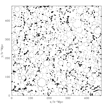
Figure 7: The distribution of voids in a $2h^{-1}$Mpc thick slice through the $512^{3}$ simulation. The positions of “wall galaxies” (in this specific case selected to be $M_{\rm b_{\rm J}}-5\log h\leq-20$ galaxies with more than three neighbours within a distance of $6.9h^{-1}$Mpc) are shown by black squares. “Void galaxies” — those with three or fewer or neighbours within the above distance — are shown as light grey squares. Voids detected using the algorithm of ? are indicate by circles. Where the void centre lies within the slice we show a solid-line circle with radius equal to the radius of the void. Where the void centre lies outside of the slice but some of the void overlaps the slice we show a dashed-line circle with radius equal to the radius of the circle where void and slice boundary intersect. Note that some wall galaxies appear to lie inside of voids due to projection effects. In reality all voids are devoid of wall galaxies.

4.1 Void Radius Distribution and Scaling Relations

Figure 8: The distribution of void radii. We plot the differential number of voids of radius $R$ per unit volume as a function of $R$. Points with errorbars show the results from our simulations, while the solid line shows the prediction from the analytical model of ?. Model results were obtained using samples of galaxies brighter than $M_{\rm b_{J}}-5\log h=-20.5$ in the GIF and $512^{3}$ simulation. We show estimates from the GIF and $512^{3}$ simulations and for dark and galaxy catalogues (symbol types as shown in the figure key). The vertical dotted line indicates the smallest radius for which the $512^{3}$ void catalogue is complete.

The simplest property of voids which we can compute is the distribution of their radii. Figure 8 shows void radii distributions for an $M_{\rm b_{J}}-5\log h\leq-20.5$ galaxy sample and the corresponding dark matter sample in both the GIF and $512^{3}$ simulations (see figure key for symbol types). Results from the $512^{3}$ simulation are incomplete for radii smaller than that indicated by the vertical dotted line, while those from the GIF simulation are complete over the whole range of radii shown. For larger voids the results from the GIF and $512^{3}$ simulations are in reasonable agreement.

Figure 8 shows, as expected from the VPF (Fig. 2), that there are more of the largest radii voids in the galaxy distribution than in the dark matter distribution. This is indicative that physical processes related to galaxy formation as well as gravity help produce voids in the galaxy distribution. At smaller radii however, the two distributions are very similar. We predict a very rapid decline in the number density of voids as their radii increase, with ${\rm d}n/{\rm d}\ln R$ falling by almost three orders of magnitude over less than half an order of magnitude in $R$. ? has derived an analytical formulae for the distribution of void sizes in the dark matter using arguments similar to those employed by ?. The distribution predicted by ? is shown in Fig. 8 by the solid line. It should be noted that in Sheth’s model a void is defined as being a region in which the interior dark matter density contrast is approximately $\Delta=\rho/\bar{\rho}=0.2$.

In contrast, our definition of voids (using the void finder) yields voids that have even lower density contrast, typically $\Delta=0.1$ or lower (especially for galaxy samples) as we will show in §4.2. As such, we should not make a direct comparison between our results and those of ?. (In particular, the analytic model of ? predicts a unique distribution, whereas our predicted distributions must necessarily depend on the density of points in our galaxy samples.) For this particular sample, the voids predicted by ? are of comparable size to those found by the void finder algorithm (typically being only 40% and 50% smaller than voids in our dark matter and galaxy catalogues respectively). More interestingly, the rapid decline in void abundance with radius seen in our model agrees well with that predicted by ?, who demonstrates that this is due to the fact that the underdense regions of the Universe from which these voids form are exponentially rare (assuming a Gaussian distribution of initial density contrasts).

In Fig. 9 we show void radii distributions for galaxy samples with different magnitude limits and selected in both b_J and r-bands. As expected, for brighter (and so sparser) samples the distribution shifts to larger sizes. The void radii distributions show evidence of a peak (especially visible in the $M_{\rm b_{J}}-5\log h\leq-20$ and $\leq-22$ panels), indicating a characteristic size for voids. Finding voids using a higher resolution grid does not change the position of this peak, indicating that it is a real feature and not an artifact due to the limited resolution of the computational grid. The limited dynamic range of the current simulations allows us to say that the position of the peak moves to larger radii as the sample of galaxies becomes brighter/sparser, but prevents us from making any more quantitative conclusions (although we can quantify the scaling of median void size with galaxy luminosity as we will show below). The presence and changing position of this peak is caused by the percolation of small voids into larger ones, a process which depends on the mean density of the sample.

Note that while the GIF simulation appears to contain systematically more large voids per unit volume than the $512^{3}$ simulation (e.g. see the third row in Fig. 9) the difference is only marginally significant. Assuming Poisson counting statistics the GIF simulation exceeds the void abundance in the $512^{3}$ simulation by $~{}\hbox to0.0pt{$<$\hss}{\lower 4.30554pt\hbox{$\sim$}}2\sigma$ for these samples. We have also computed void radii distributions using the GIF-II simulation (described in §2). We find that the Poisson errors are a reasonable representation of the differences between the results from the GIF and GIF-II simulations, while the GIF-II results are somewhat closer to those of the $512^{3}$ simulation.

? also predicts the clustering properties of voids (specifically their bias on large scales and defined in terms of the two-point correlation function). Even with the large volume of our simulations measuring void clustering is quite difficult. On scales comparable to the void radii we find a strong anti-correlation since the void finder algorithm allows voids to overlap by at most 10% in volume. On larger scales we typically find that voids have a close to uniform distribution. However, given the small amplitude of both void and dark matter correlation functions on these scales it is impossible to make strong statements about the void bias, or how it scales with void radius, from our current simulations.

Figure 9: The distribution of void radii. We plot the differential number of voids of radius $R$ per unit volume as a function of $R$. Points with errorbars show the results from our simulations. Left hand panels show samples selected by their b_J-band magnitude, while right-hand panels show samples selected by their r-band magnitude (the magnitude selection is shown in each panel). Open and filled symbols show results from the GIF and $512^{3}$ simulations respectively. Squares and circles show results for galaxies and dark matter respectively. The vertical dotted line shows the completeness limit for the $512^{3}$ simulation. The GIF simulation is complete for the whole range of radii shown.

Figure 10: The median void radius, $R$, as a function of mean inter-galaxy separation, $\lambda$. The left-hand panel shows results for galaxies selected by their b_J-band magnitude (as appropriate to the 2dFGRS), with the right-hand panel showing results for galaxies selected by their r-band magnitude (as appropriate to the SDSS). Open symbols show results for dark matter catalogues, while filled symbols show results for galaxy catalogues. Circles and squares show results from the GIF and $512^{3}$ simulations respectively. Errorbars enclose 50% of the distribution of void radii. Horizontal dotted lines indicate the completeness limit for each simulation. The solid line indicates the best fit linear relation to the galaxy results, including only those points for which more than 75% of the voids have radii greater than the completeness limit.

? show that voids in redshift surveys and in mock galaxy catalogues built from CDM simulations obey a simple scaling relation, such that the median void radius, $R$, obeys $R=R_{0}+\nu\lambda$, where $\lambda$ is the mean galaxy separation of the sample in question and $R_{0}$ and $\nu$ are parameters. In Fig. 10 we show the $R$–$\lambda$ relation for voids in our simulations. We compute $R$ for all the galaxy samples using both the GIF and $512^{3}$ simulations. Note that there is little difference seen in the median void size between galaxy and dark matter samples. The differences in the void size distribution seen in Fig. 8 occur only for the largest voids, which have very low number density and so have little impact on the median void size. The parameters $R_{0}$ and $\nu$ are determined using a least squares fit, including only those points for which 75% of the voids in the sample have radii in excess of the completeness limit for the simulation in question. For the 2dFGRS sample we find $R_{0}=-0.11\pm 0.6$ and $\nu=1.42\pm 0.04$, while for the SDSS sample we find $R_{0}=-0.06\pm 0.2$ and $\nu=1.40\pm 0.02$. Thus, the scaling relations for our two samples are consistent within the errorbars. Our results differ somewhat from those of ?, who find higher values of $\nu$, and larger values of $R_{0}$ for CDM mock galaxy catalogues constructed using a simple biassing scheme and for the Las Campanas Redshift Survey. This is not surprising given that we employ a different void finding algorithm, but does serve to highlight the importance of analyzing model and observations using the same algorithm. Nevertheless, such a linear scaling relation with slope $\nu>1$ is found in both void detection schemes, suggesting that it may be a generic feature of the void distribution.

4.2 Void Density Profiles

In the void finder algorithm voids need not be entirely devoid of galaxies. Galaxies with few nearby neighbours are classified as “void galaxies” and may be located within the subsequently detected voids. To assess the prevalence of such galaxies, and the larger scale structure surrounding voids, we have determined void density contrast profiles from our simulations. To do this we determine the number density of galaxies in concentric shells centred on each void centre, scaling all length scales by the void radius to allow us to compare voids of different sizes. We sum the resulting number density profiles over all voids in a particular range of radii and convert this into a density contrast profile. The results of this procedure are shown in Fig. 11.

Figure 11: Mean density contrast as a function of radial position in voids. We plot the mean density contrast as a function of scaled radius (i.e. we express radius in each void in units of the void radius) and averaged over all voids in our GIF and $512^{3}$ simulations (left and right-hand panels respectively). Left and right-hand panels show results for voids found in galaxy samples selected to have $M_{\rm b_{J}}-5\log h\leq-19.5$ and $-20.5$ respectively. Upper, middle and lower panels include those voids with radii larger than $15$, $17.5$ and $20h^{-1}$Mpc respectively. Open circles show results for dark matter catalogues, while filled circles show results for galaxy catalogues.

We show results for both galaxy and dark matter catalogues (filled and open points respectively), for a range of minimum void sizes and for two different magnitude selections (as indicated in the panels). Voids are highly underdense, galaxy voids more so than dark matter voids (typically density contrasts are $0.1$ and $0.2$ respectively for the $M_{\rm b_{J}}-5\log h\leq-20.5$ sample), again demonstrating the biasing of galaxies relative to dark matter (this can be seen most clearly in the upper left-hand panel of Fig. 11). There is little variation in density contrast within much of the void, but there is evidence for a decline in density contrast in the very central regions of the voids. There is a clear threshold corresponding to the edge of each void which occurs close to $r/R_{\rm void}=1$, especially for the $M_{\rm b_{J}}-5\log h\leq-20.5$ sample, indicating that the void finder algorithm is working successfully. Beyond the void radius we find the density contrast increases rapidly (more rapidly for galaxies than dark matter), but can remain below unity for a significant distance. Thus, for our $M_{\rm b_{J}}-5\log h\leq-20.5$ sample the regions around voids are, on average, still underdense even at twice the void radius. These findings are in qualitative agreement with the void density profiles reported by ?, with the exception that our voids are less dense (for both galaxies and dark matter), and their boundaries are sharper (i.e. density contrast increases more rapidly beyond the void radius). This is again a consequence of the differing algorithms for defining voids in the two approaches, highlighting the importance of analysing observations and theoretical models in identical ways.

5 Properties of Void Galaxies

Figure 12: Normalized distributions of b_J/r-band absolute magnitude, B$-$V/g$-$r colour, bulge-to-total ratio (measured in dust-extinguished b_J-band light) and star formation rate (top to bottom panels respectively) for 2dFGRS/SDSS samples for the general population of galaxies (dotted histograms) and galaxies living inside voids of radius 12.5Mpc/h or larger (solid histograms with error bars indicating the Poisson variation). In all cases we limit the sample of galaxies to those brighter than b${}_{\rm J}-5\log h\leq-19$ and ${\rm r}-5\log h\leq-20$ for 2dFGRS and SDSS samples respectively. The fraction of galaxies in these samples which live in such voids, $f_{\rm void}$, is shown at the bottom of the figure. All results are from the GIF simulation.

In Fig. 12 we show, for the GIF simulation, the distributions of galaxy luminosities, colours, morphologies and star formation rates for both the general population (dotted histograms) and for galaxies living within voids (i.e. those galaxies lying within the spherical voids found using the void finder; solid histograms). Note that the fraction of galaxies which are actually located within voids (shown at the bottom of Fig. 12) is much lower than the fraction of galaxies classified as “void galaxies” by the void finder algorithm. A similar result is found for the observational samples employed by ?. It is clear that void galaxies have systematically different properties to the general population—although the differences are typically rather small (similar results are found in the $512^{3}$ simulation). Nevertheless, a Kolmogorov-Smirnov test indicates that the void and field galaxy samples are inconsistent with being drawn from a single underlying distribution (the probability being less than 6% in all cases). Void galaxies are typically fainter and bluer, are more disk-dominated and show higher star formation rates. All of these differences can be traced to the difference in dark matter halo mass functions in voids (indeed, in our model, this is the only possible means of creating a difference between voids and the general field). For example, in the field some fraction of galaxies fall into clusters where their supply of fresh gas is “strangled” (i.e. their diffuse halos of hot gas is removed by the ram pressure and tidal forces due to the cluster), resulting in a cessation of star formation. Since there are no clusters in voids this process is far less important for void galaxies.

For the samples shown in Fig. 12 the halo mass function (for halos occupied by one of the galaxies) is shown in Fig. 13. Clearly the halo mass function of void galaxies (solid line) is shifted to much lower masses relative to that of the field sample (dotted line). The median occupied halo mass is over 6 times lower for void galaxies than for field galaxies. The majority of these void galaxies live at the centre of their halo, whereas in the general population we find a large fraction of the galaxies existing as satellites in more massive halos.

Figure 13: The (galaxy number weighted-)dark matter halo mass function for a sample of $M_{\rm b_{J}}-5\log h\leq-19$ galaxies from the GIF simulation. The dotted line shows that of all such galaxies, while the solid line shows the result for galaxies living inside voids of radius $12.5h^{-1}$Mpc or larger.

We are also able to explore how the star formation rate of galaxies varies with radius inside voids. In Fig. 14 we show the mean specific star formation rate (i.e. the star formation rate per unit mass of stars) in model galaxies as a function of their normalized distance from the nearest void centre, where we include only voids larger than a particular radius (as indicated in the figure). Results are shown for two b_J-band selected samples as indicated in the figure (the fainter one drawn from the GIF simulation, the brighter one from the $512^{3}$ simulation). Results for the full samples of galaxies are shown by the filled points. There is a clear trend for higher specific star formation rates as we move towards the centres of voids (for the fainter sample in particular, the trend is seen out to twice the void radius). There are two contributions to this effect. Firstly, outside of voids we find very massive halos which contain large populations of satellite galaxies. In our model these galaxies have lost their supply of fresh gas, and so star formation is strongly suppressed in these systems. Since such massive halos are very rare in voids the majority of void galaxies are the dominant galaxy of their halo, so retain a gas supply allowing higher rates of star formation. We can see the contribution of this effect by repeating this calculation using only central galaxies (i.e. those with a continued gas supply), as shown by the open symbols in Fig. 14. For the fainter sample in particular this can be seen to be the dominant contributor to the trend. A secondary contributor to the trend is that, even for galaxies with a continued gas supply, specific star formation rates tend to be higher for lower mass galaxies in our model. This weaker trend is visible in the open symbols in Fig. 14.

Figure 14: The specific star formation rate (i.e. the star formation rate per unit mass of stars) in model galaxies as a function of the radius relative to their nearest void centre. The mean specific star formation rate is plotted for two different luminosity selections (squares and circles, as indicated in the figure) as a function of normalized radius to the nearest void centre. Filled symbols include all model galaxies in the specified luminosity range, while open symbols include only those living at the centre of their halo (i.e. it excludes satellite galaxies). Results are computed for voids larger than $10$ and $15h^{-1}$Mpc for the faint and bright samples respectively.

Larger differences may occur for fainter samples of galaxies, below the resolution limit of our simulations. If faint field galaxies exist mostly as satellites in massive groups and clusters (which are not located in voids) then significant differences between field and void samples could occur. If, on the other hand, faint field galaxies exist mostly in lower mass halos (where the differences between field and void halo mass functions are much smaller) we would expect the differences to be smaller also. Benson et al. (in preparation) examine the relative contributions of satellite and non-satellite galaxies to the galaxy luminosity function, finding that satellites become the dominant contribution faintwards of $M_{\rm B}-5\log h\approx-16.5$, suggesting that we would need to probe over two magnitudes fainter than currently possible to see significant differences between void and field galaxies.

6 Discussion

We have presented detailed theoretical predictions for a wide range of statistics related to voids in the distribution of galaxies, and for properties of galaxies living within those voids. These predictions have been specifically aimed at the 2dFGRS and SDSS, which, due to their large size, should provide accurate measures of these statistics. We have focussed on simple selection criteria, namely simple cuts in luminosity, which we believe will permit the most robust comparison between theory and observations.

The properties of voids and void galaxies are potentially a strong constraint on models of structure and galaxy formation. However, we have shown that many of the properties of galaxy and dark matter voids differ significantly, indicating (as we have shown) that galaxy bias as well as gravitational instability is important for the formation of galaxy voids. Although our understanding of galaxy bias has progressed greatly in recent years we cannot be certain that our understanding is complete. Where suitable data already exist (specifically the void and underdense probability functions analysis applied to the CfA surveys by ?) we find that the model is consistent with the data, but that the current observational sample is too small to probe the signal of bias expected from our model. This situation should be rectified when this analysis is repeated on larger redshift surveys.

As has been shown in previous works on galaxy clustering using semi-analytic and N-body techniques, the results are rather robust to changes in model parameters (?). If we compute void statistics such as the VPF, nearest neighbour distributions or void size distributions at a fixed number density then our predictions are unaffected by changes in most model parameters (e.g. the strength of supernovae feedback, the star formation timescales in galaxies etc.). This results from the fact that the main effect of changing these parameters is to change galaxy luminosities without significantly changing the ranking of galaxy luminosity. Predictions are changed by parameters in the model which do change the ranking of luminosities. For example, significantly increasing or decreasing the rates of galaxy mergers can make strong differences in some of the statistics considered here. (Note however, that with the improved merging model of ? we no longer have the freedom to adjust merger rates in our model.) The properties of void galaxies (e.g. Fig. 12) are affected by changes in model parameters. As the differences between void and wall galaxies seen in Fig. 12 are so small we choose not to explore the dependencies of these properties on model parameters in this work.

The models employed in our analysis include the effects of “photoionization suppression” as described by ?. This feedback mechanism has the potential to strongly alter the properties of voids in the galaxy distribution. Halos in voids are of lower mass on average than in higher density regions. Since photoionization suppression acts most effectively on low-mass halos it will cause greatest suppression of galaxy formation in voids. (Furthermore, although not included in our present modelling, reionization of the Universe may begin in voids, enhancing the suppression in these regions further.) For the lowest mass galaxies resolved in our current N-body simulations the effects of photoionization suppression are negligible (e.g. the VPF and nearest neighbour distributions for galaxy samples of fixed number density are indistinguishable between models with and without photoionization suppression). We may expect however strong differences to show up in higher resolution simulations.

References

- [Amendola et al. ¡1999¿] Amendola L., Baccigalupi C., Gleiser M., Occionero F., 1999, New Astronomy, 3, 339
- [Arbabi-Bidgoli & Müller ¡2002¿] Arbabi-Bidgoli S., Müller V., 2002, MNRAS, 332, 205
- [Benson et al. ¡2000a¿] Benson A. J., Cole S., Frenk C. S., Baugh C. M., Lacey C. G., 2000a, MNRAS, 311, 793
- [Benson et al. ¡2000b¿] Benson A. J., Baugh C. M., Cole S., Frenk C. S., Lacey C. G., 2000b, MNRAS, 316, 10
- [Benson et al. ¡2001¿] Benson A. J., Frenk C. S., Baugh C. M., Cole S., Lacey C. G., 2001, MNRAS, 327, 1041
- [Benson ¡2001¿] Benson A. J., 2001, MNRAS, 325, 1039
- [Benson et al. ¡2002a¿] Benson A. J., Lacey C. G., Baugh C. M., Cole S., Frenk C. S., 2002a, MNRAS, 333, 156
- [Benson et al. ¡2002b¿] Benson A. J., Lacey C. G., Baugh C. M., Cole S., Frenk C. S., 2002b, in preparation
- [Blanton et al. ¡2001¿] Blanton M. R. et al., 2001, ApJ, 121, 2358
- [Cen & Ostriker ¡2000¿] Cen R., Ostriker J. P., 2000, ApJ, 538, 83
- [Cole et al. ¡2000¿] Cole S., Lacey C. G., Baugh C. M., Frenk C. S., 2000, MNRAS, 319, 168
- [Davis & Geller ¡1976¿] Davis M., Geller M. J., 1976, ApJ, 208, 1
- [Einasto et al. ¡1991¿] Einasto J., Einasto M., Gramann M., Saar E., 1991, 248, 593
- [El-Ad & Piran ¡1997¿] El-Ad H., Piran T., 1997, ApJ, 491, 421
- [Geller & Huchra ¡1989¿] Geller M. J., Huchra J. P., 1989, Science, 246, 897
- [Ghigna et al. ¡1994¿] Ghigna S., Borgani S., Bonometto S. A., Guzzo L., Klypin A., Primack J. R., Giovanelli R., Haynes M. P., 1994, ApJ, 437, 71
- [Ghigna et al. ¡1996¿] Ghigna S., Bonometto S. A., Retzlaff J., Gottlöber S., Murante G., ApJ, 469, 40
- [Gregory & Thompson ¡1978¿] Gregory S. A., Thompson L. A., 1978, ApJ, 222, 784
- [Hoyle et al. ¡1999¿] Hoyle F., Baugh C. M., Shanks T., Ratcliffe A., 1999, MNRAS, 309, 659
- [Hoyle & Vogeley ¡2002¿] Hoyle F., Vogeley M. S., 2002, ApJ, 566, 641
- [Jenkins et al. ¡2001¿] Jenkins A., Frenk C. S., White S. D. M., Colberg J. M., Cole S., Evrard A. E., Couchman H. M. P., Yoshida N., 2001, MNRAS, 321, 372
- [Kauffmann, Nusser & Steinmetz ¡1997¿] Kauffmann G., Nusser A., Steinmetz M., 1997, MNRAS, 286, 795
- [Kauffmann et al. ¡1999¿] Kauffmann G., Colberg J. M., Diaferio A., White S. D. M., 1999, MNRAS, 303, 188
- [Kirshner et al. ¡1981¿] Kirshner R. P., Oemler A. Jr., Schechter P. L., Shectman S. A., 1981, ApJ, 248, L57
- [Little & Weinberg ¡1994¿] Little B., Weinberg D. H., 1994, MNRAS, 267, 605
- [Mathis & White ¡2002¿] Mathis H., White S. D. M., 2002, submitted to MNRAS (astro-ph/0201193)
- [Müller et al. ¡2000¿] Müller V., Arbabi-Bidgoli S., Einasto J., Tucker D., 2000, MNRAS, 318, 280
- [Norberg et al. ¡2001a¿] Norberg P. et al., 2001a, MNRAS, 328, 64
- [Norberg et al. ¡2002¿] Norberg P. et al., 2002, MNRAS, 332, 827
- [Ostriker & Cowie ¡1981¿] Ostriker J. P., Cowie L. L., 1981, ApJ, 243, L127
- [Peebles ¡2001¿] Peebles P. J. E., 2001, astro-ph/0101127
- [Press & Schechter ¡1974¿] Press W. H., Schechter P., 1974, ApH, 187, 425
- [Sheth ¡2002¿] Sheth R. K., 2002, submitted to MNRAS
- [Verde et al. ¡2002¿] Verde L. et al., 2002, submitted to MNRAS (astro-ph/0112161)
- [Vogeley et al. ¡1991¿] Vogeley M. S., Geller M. J., Huchra J. P., ApJ, 1991, 382, 44
- [Vogeley et al. ¡1994¿] Vogeley M. S., Geller M. J., Park C., Huchra J. P., 1994, AJ, 108, 745
- [White ¡1979¿] White S. D. M., 1979, MNRAS, 186, 145
- [Zehavi et al. ¡2002¿] Zehavi I. et al. (the SDSS Collaboration), ApJ, 571, 172
- [Zehavi et al. ¡2003¿] Zehavi I. et al., in preparation