Dark Synergy: Gravitational Lensing and the CMB

Abstract

Power spectra and cross-correlation measurements from the weak gravitational lensing of the cosmic microwave background (CMB) and the cosmic shearing of faint galaxies images will help shed light on quantities hidden from the CMB temperature anisotropies: the dark energy, the end of the dark ages, and the inflationary gravitational wave amplitude. Even with modest surveys, both types of lensing power spectra break CMB degeneracies and they can ultimately improve constraints on the dark energy equation of state $w$ by over an order of magnitude. In its cross correlation with the integrated Sachs-Wolfe effect, CMB lensing offers a unique opportunity for a more direct detection of the dark energy and enables study of its clustering properties. By obtaining source redshifts and cross-correlations with CMB lensing, cosmic shear surveys provide tomographic handles on the evolution of clustering correspondingly better precision on the dark energy equation of state and density. Both can indirectly provide detections of the reionization optical depth and modest improvements in gravitational wave constraints which we compare to more direct constraints. Conversely, polarization B-mode contamination from CMB lensing, like any other residual foreground, darkens the prospects for ultra-high precision on gravitational waves through CMB polarization requiring large areas of sky for statistical subtraction. To evaluate these effects we provide fitting formula for the evolution and transfer function of the Newtonian gravitational potential.

]

I Introduction

With the launch of the MAP satellite and continuing progress in ground and balloon based experiments, cosmologists hope to soon be in a situation where cosmic microwave background (CMB) anisotropies have firmly established the adiabatic cold dark matter paradigm for structure formation and the parameters that govern it at high redshift. Attention on the experimental and theoretical front will increasingly turn to the potentially deeper questions at the two opposite ends of time: the energy contents of the universe and their clustering properties at recent epochs and the origins of structure perhaps in the inflationary epoch. From distance measures to high redshift supernova [2] and indications of a near critical density universe from the CMB [3], there is increasingly strong evidence for an unknown component of dark energy that accelerates the expansion at low redshifts.

In this context, it is useful to consider potential cosmological probes in light of what the primary CMB temperature anisotropies are and are not expected to reveal. While some parameters such as the physical baryon and non-relativistic matter density should be quite cleanly determined, others such as the dark energy properties, the epoch of reionization, and the gravitational wave amplitude are entangled with each other in parameter degeneracies. While the CMB polarization is one well-recognized means of breaking some of these degeneracies, these issues are sufficiently important and polarization measurements sufficiently difficult that multiple independent approaches are desirable.

In this Paper, we compare and contrast the ability of weak gravitational lensing in the shearing of faint galaxy images and distortions of the CMB temperature anisotropies in shedding light on these issues in the post-primary CMB epoch. Weak gravitational lensing shares with the primary anisotropies a unique status in cosmology in that its observables are in principle predictable ab initio given a cosmological model. Measurements are limited mainly by instrumental systematics rather than unknown astrophysics. As such lensing observables are well-suited to complement information from the CMB.

Recent works [4, 5, 6] have shown that it is possible to map structures on the largest scales at high redshift through the lensing of the CMB. We evaluate here the utility of such measurements and their cross-correlation with the anisotropies themselves as well as cosmic shear for cosmological parameter estimation. On the cosmic shear side, we extend the work of [7] by considering correlations with CMB temperature anisotropies and lensing. We also utilize the extended parameter space of [8] to study the background and clustering properties of the dark energy. In this context, Huterer [9] has recently shown that the sub-arcminute regime provides substantial information on the dark energy but will require a better understanding of the power spectrum and its statistical properties in the deeply non-linear regime (e.g. [10]). Here we take the complementary tack of supplementing information in the translinear regime with source redshift information [11].

The outline of the paper is as follows: in §II we describe the the cosmological parameter space, power spectra and cross correlations of the observables and the Fisher formalism for parameter estimation forecasts. In §III, we discuss the phenomenology of the lensing observables and their utility in breaking cosmological parameter degeneracies. We present parameter forecasts in §IV and conclude in §V. In the Appendix, we give fitting formula for the transfer function and evolution of the Newtonian curvature in the presence of the dark energy.

II Formalism

We begin in §II A by defining the cosmological context paying special care to define quantities properly in the presence of dark energy. In §II B we review the harmonic formalism for handling scalar, vector and tensor fields on the sky and consider the calculation of their power spectra and cross correlations in §II C. Finally we generalize the Fisher formalism for multiple observables from overlapping fields in §II D.

A Cosmological Parameters

We work in the context of spatially flat cold dark matter models for structure formation with initial curvature fluctuations. In units of the total (critical) density $3H^{2}/8\pi G$, with $c=1$, the fractional contribution of each component is denoted $\Omega_{i}(z)$, $i=c$ for the CDM, $b$ for the baryons and $\Lambda$ for the dark energy. We also define the auxiliary quantity $\Omega_{m}=\Omega_{c}+\Omega_{b}$, the total non-relativistic matter. We assume throughout that the neutrinos contribute negligible matter density. The expansion rate at epochs where the radiation is negligible is given by

$$H^{2}=H_{0}^{2}[\Omega_{m}(0)(1+z)^{3}+\Omega_{\Lambda}(0)\rho_{\Lambda}(z)/\rho_{\Lambda}(0)]\,,$$ (1)

where $H_{0}=100h$ km s^-1 Mpc^-1 is the Hubble constant. The evolution of the dark energy density is governed by its equation of state $w=p_{\Lambda}/\rho_{\Lambda}$ such that

$$\rho_{\Lambda}^{\prime}=-3(1+w)\rho_{\Lambda}\,,$$ (2)

where ^′ denotes a derivative with respect to $\ln(1+z)^{-1}$. For illustrative purposes, we take $w=$ const. such that $\rho_{\Lambda}(z)=\rho_{\Lambda}(0)(1+z)^{3(1+w)}$. Thus 4 parameters are associated with background energy densities $\Omega_{b}h^{2}$, $\Omega_{m}h^{2}$, $\Omega_{\Lambda}$ and $w$ all evaluated at the present epoch. We will often use the conformal lookback time in lieu of the redshift

$$D(z)=\int_{0}^{z}{dz^{\prime}\over H(z^{\prime})}\,,$$ (3)

abusing notation in the arguments of functions where no confusion will arise. Overdots will represent derivatives with respect to $D$ throughout. The final parameter associated with the background cosmology is the Thomson optical depth in the reionization epoch $\tau$.

Four parameters are associated with the perturbations to the background. An amplitude and a tilt define the initial fluctuations in the logarithmic power spectrum of the Bardeen or comoving gauge curvature $\zeta$ [12]

$$\langle\zeta({\bf k},z)\zeta({\bf k}^{\prime},z)\rangle=(2\pi)^{3}\delta({\bf k}-{\bf k}^{\prime}){2\pi^{2}\over k^{3}}\Delta_{\zeta}^{2}(k,z)\,,$$ (4)

as

$$\Delta_{\zeta}^{2}(k,z_{i})=\delta_{\zeta}^{2}\left({k\over k_{\rm fid}}\right)^{n-1}\,,$$ (5)

where the fiducial scale is taken to be $k_{\rm fid}=0.01$ Mpc^-1 and the initial (or inflationary) epoch $z_{i}$ is taken to be sufficiently early that all relevant scales are outside the horizon. Under slow roll inflation (e.g. [13]),

$$\Delta_{\zeta}^{2}(k,z_{i})={8\over 3\epsilon}{V\over m_{\rm pl}^{4}}\,,$$ (6)

where $m_{\rm pl}$ is the Planck mass and $\epsilon={3\over 2}(1+w_{i})$ is the deviation from vacuum domination in the equation of state of the inflaton, all evaluated when the relevant scale exited the horizon.

The Bardeen curvature provides a convenient representation since it remains constant outside the horizon in a flat universe regardless of its energy contents. It is related to the power spectrum of Newtonian curvature fluctuations as

$$\Delta_{\Phi}^{2}(k,z)=\Phi_{c}^{2}(z){T_{w}(k,z)\over T_{w}(0,z)}T_{m}(k)\Delta_{\zeta}^{2}(k,z_{i})$$ (7)

in the linear regime. The potential decay function in the large-scale limit $\Phi_{c}$ and transfer functions $T_{w}$ and $T_{m}$ are given in the Appendix. The partitioning of the transfer function into two pieces reflects its relationship to the matter density fluctuations $\Delta_{m}^{2}$ in the comoving gauge

$$\Delta_{\Phi}^{2}(k,z)={9\over 4}\left({H_{0}\over k}\right)^{4}\Omega_{m}^{2}(0)(1+z)^{2}\Delta_{m}^{2}(k,z)\,,$$ (8)

where

$$\Delta_{m}^{2}(k,z)\approx\delta_{H}^{2}\left({k\over H_{0}}\right)^{3+n}\left(T_{w}(k,z){T_{m}(k)\over 1+z}{\Phi_{s}(z)\over\Phi_{s}(0)}\right)^{2}\,,$$ (9)

under the approximation that the comoving dark energy density fluctuation contributes negligibly to the Newtonian curvature. Here $\Phi_{s}$ is the potential decay function in the small scale limit where dark energy clustering is negligible. Note that in the presence of dark energy with $w>-1$, the transfer function in the comoving gauge is no longer equivalent to that in the synchronous gauge on scales approaching $1/H(z)$ during dark energy domination. The factor $T_{w}(k,z)$ given in the Appendix accounts for dark energy clustering in the comoving gauge (c.f. [15]). $T_{m}$ is the usual matter transfer function defined in the absence of dark energy clustering and is here numerically evaluated to $k\approx 0.5h$ Mpc^-1 and extended to smaller scales with the fitting functions of [14]. We use the PD96 [16] scaling relations for $\Delta_{m}^{2}$ and the decay function $\Phi_{s}(D)$ to extend the potential power spectrum into the non-linear regime.

These relations also give the mapping between our normalization scheme and the more traditional one

$$\delta_{H}\approx{2\over 3}\left({k_{\rm fid}\over H_{0}}\right)^{{1-n}\over 2}{\Phi_{s}(0)\over\Omega_{m}(0)}\delta_{\zeta}\,.$$ (10)

We allow for scale-invariant initial tensor or gravitational wave fluctuations. In the notation of [17], where $H^{(\pm 2)}=(h_{+}\mp ih_{\times})/\sqrt{6}$ represent the amplitudes of the two polarizations in spin modes, the power spectrum in each component is given by (e.g. [13])

$$\Delta_{H}^{2}(k,z_{i}) = \delta_{T}^{2}\left({k\over k_{\rm fid}}\right)^{n_{T}}={32\over 9}{V\over m_{\rm pl}^{4}}\,.$$ (11)

We take $n_{T}=0$ throughout.

Finally, we take one parameter for the equation of state for the perturbations in the dark energy. Because the dark energy has negative pressure, pressure fluctuations cannot be adiabatically related to density fluctuations through the equation of state. Following [18], we take

$$c_{\rm eff}^{2}\equiv{\delta p\over\delta\rho}\Big{|}_{\rm rest}\,,$$ (12)

to be the sound speed of the dark energy in its rest frame where its energy flux vanishes. During dark energy domination the rest frame and the comoving frame coincide. The dark energy can be considered smooth on scales smaller than the distance sound can travel. If the dark energy is composed of a single slowly rolling scalar field [19], $c_{\rm eff}=1$ and the sound horizon coincides with the particle horizon. Because the horizon at high redshift decreases, the clustering of the dark energy can leave an imprint on observable scales even for a scalar field. Measurement of this imprint can therefore test the scalar field paradigm for dark energy (see §IV D). Note that as $w\rightarrow-1$, the phenomenological consequence of $c_{\rm eff}$ disappears due to the vanishing of the relativistic energy flux $(\rho_{\Lambda}+p_{\Lambda})v_{\Lambda}\rightarrow 0$. Dark energy candidates necessarily become indistinguishable from a true cosmological constant in this limit.

This family of models is therefore described by 9 parameters. We take as our fiducial choices: $\Omega_{b}h^{2}=0.02$, $\Omega_{m}h^{2}=0.148$, $\Omega_{\Lambda}=0.65$, $w=-1$ or $-2/3$, $\tau=0.05$, $\delta_{\zeta}=4.79\times 10^{-5}$, $n=1$, $\delta_{T}=0$, $c_{\rm eff}^{2}=1$. It is conventional to express the tensor amplitude in terms of the scalar amplitude normalized to their individual contributions to the CMB temperature quadrupole. Note that the normalization is dependent on cosmological parameters, especially the dark energy [20], and we take the scaling appropriate to the $w=-1$ fiducial model:

$${T\over S}\Big{|}_{\rm fid} = \left({\delta_{T}\over 1.85\times 10^{-5}}\right)^{2}\,,$$ (13)

$$= \left({V^{1/4}\over 3.9\times 10^{16}{\rm GeV}}\right)^{4}\,.$$ (14)

With this relation, $T/S$ constraints can be converted to tensor amplitude and inflationary energy scale constraints.

B Observables and Power Spectra

CMB and lensing observables are described by scalar, vector and tensor fields on the sky. A general scalar field on the sky $S(\hat{\bf n})$, where $\hat{\bf n}$ is the directional vector, is decomposed into multipole moments of the spherical harmonics as

$$S(\hat{\bf n})=\sum_{lm}S_{lm}Y_{l}^{m}(\hat{\bf n})\,.$$ (15)

Similarly a vector field ${\bf V}(\hat{\bf n})=(V_{1},V_{2})$ is decomposed as

$$[V_{1}\pm iV_{2}](\hat{\bf n})=\sum_{lm}(P_{lm}\pm iS_{lm})\,{}_{\pm 1}Y_{l}^{m}(\hat{\bf n})\,,$$ (16)

where $S_{lm}$ is the curl-free part and $P_{lm}$ is the divergence-free part. Here ${}_{s}Y_{lm}$ are the spin-spherical harmonics [21]. Finally a trace free tensor field can be represented with the Pauli matrices ${\bf\mbox{\boldmath$\sigma$}}_{i}$

$${\bf T}(\hat{\bf n})=T_{1}{\bf\mbox{\boldmath$\sigma$}}_{1}+T_{2}{\bf\mbox{\boldmath$\sigma$}}_{2}+T_{3}{\bf\mbox{\boldmath$\sigma$}}_{3}\,;$$ (17)

the trace behaves as a scalar field. The symmetric part can be further decomposed as

$$[T_{3}\pm iT_{1}](\hat{\bf n})=\sum_{lm}(S_{lm}\pm iP_{lm})\,{}_{\pm 2}Y_{l}^{m}(\hat{\bf n})\,.$$ (18)

For the tensor case $S_{lm}$ is often called the “electric” or “$E$” and $P_{lm}$ the “magnetic” or “$B$” component of the field. The remaining piece can be decomposed as

$$T_{2}(\hat{\bf n})=\sum_{lm}P_{lm}Y_{l}^{m}(\hat{\bf n})\,,$$ (19)

and is called the circular mode. As the notation implies, the harmonics of the gradient and electric components can be written in terms of those of a scalar potential field on the sky; the curl, magnetic and circular modes can be written in terms of the harmonics of a pseudo-scalar field.

Statistical isotropy guarantees that the for any of two sets of harmonics $X=S,$ $P$

$$\left<X_{lm}^{*}X^{\prime}_{l^{\prime}m^{\prime}}\right> = \delta_{l,l^{\prime}}\delta_{m,m^{\prime}}C_{l}^{XX^{\prime}}\,,$$ (20)

which defines the power spectra. Parity invariance requires that cross-spectra between scalar and pseudo scalar types vanish.

C Tracer Fields

In the linear regime, all scalar fields on the sky that are related to cosmological structures can be thought of as line-of-sight projections of the gravitational potential $\Phi({\bf x},D)$ with a suitable weight

$$X(\hat{\bf n})=\int dD\,W^{X}(D)\Phi(D\hat{\bf n},D)\,,$$ (21)

where $W$ can include differential operators on the potential field. In the non-linear regime, any tracer of the density fluctuations may also be treated as such. The scalar piece of vector and tensor fields can then also be reduced to this form.

Taking the harmonic moments of Eqn. (21) yields,

$$X_{lm} = 4\pi i^{l}\int{d^{3}k\over(2\pi)^{3}}\Phi({\bf k},0)I_{l}^{X}(k)Y_{l}^{m}(\hat{\bf k})\,,$$ (22)

$$I_{l}^{X}(k) = \int dD\,{\Phi(k,D)\over\Phi(k,0)}W^{X}(k,D)j_{l}(kD)\,.$$ (23)

The power spectrum of two fields then becomes

$$C_{l}^{XX^{\prime}}=4\pi\int{dk\over k}I_{l}^{X}(k)I_{l}^{X^{\prime}}(k)\Delta_{\Phi}^{2}(k,0)\,,$$ (24)

and can be reexpressed in terms of the initial spectrum $\Delta_{\zeta}^{2}(k,z_{i})$ through Eqn. (7). For the CMB, this technique is known as the integral approach to anisotropies [23].

In the Limber approximation limit [22], $k\gg\dot{W}^{X}/W^{X}$ and $l\gg 1$,

$$I_{l}^{X}(k)\approx\sqrt{\pi\over 2l}{1\over k}{\Phi(k,l/D)\over\Phi(k,0)}W^{X}(k,l/k)\,,$$ (25)

and with a change of variables $D=l/k$ the power spectrum becomes

$$C_{l}^{XX^{\prime}}={2\pi^{2}\over l^{3}}\int dD\,DW^{X}(D)W^{X^{\prime}}(D)\Delta_{\Phi}^{2}(k,D)\,.$$ (26)

We will use these equations to calculate the power spectra and cross correlations of the various effects.

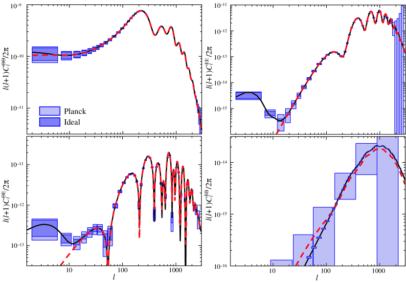
FIG. 1.: CMB power spectra in the fiducial model with $w=-1$ (solid) versus a dark energy model with $w=-2/3$ (dashed) and other parameters chosen to preserve the angular diameter distance and amplitude degeneracies (see text). Boxes represent $1\sigma$ errors on band powers for the Planck experiment and an ideal experiment out to $l=3000$ (see Tab. I).

D Fisher Matrix

If all fields are Gaussian random, then the power and cross spectra quantify all the information contained in the observables. We can then use Fisher matrix techniques to combine, compare and contrast the statistical precision to which various surveys can determine the parameters underlying the power spectra.

The Fisher matrix approximates the curvature of the likelihood function around its maximum in a space spanned by the parameters ${\bf p}$ such that the statistical errors on a given parameter $p_{\alpha}$: $\sigma(p_{\alpha})\approx({\bf F}^{-1})_{\alpha\alpha}$. The usual formulae (e.g. [24]) require a slight generalization to account for the possibility that different surveys may only partially overlap in sky coverage. For the $i$th patch of sky, the elements of the Fisher matrix are given by

$$F_{\alpha\beta}^{i}=\sum_{l_{\rm min}}^{l_{\rm max}}(l+1/2)f_{\rm sky}^{i}{\rm Tr}[{\bf C}^{-1}{\bf C}_{,\alpha}{\bf C}^{-1}{\bf C}_{,\beta}]\,,$$ (27)

Here $,\alpha=\partial/\partial p_{\alpha}$ and ${\bf C}$ is the covariance matrix of the multipole moments of the observables

$${\bf C}_{XX^{\prime}}=C_{l}^{XX^{\prime}}+N_{l}^{XX^{\prime}}$$ (28)

where $N_{l}^{XX^{\prime}}$ is the power spectrum of the noise in the measurement. $f_{\rm sky}^{i}$ is the fraction of sky in the patch and quantifies the loss of independent modes due to finite sky coverage. We take $l_{\rm min}=0.5f_{\rm sky}^{-1/2}$; the precise definition does not matter due to the increase in sample variance on the scale of the survey. Although formally $l_{\rm max}\rightarrow\infty$, we generally take $l_{\rm max}=3000$. Above this scale non-Gaussianity in both the CMB and lensing fields begin to violate the assumptions behind the Fisher formalism.

Under the approximation that each patch is statistically independent, the full Fisher matrix is the sum of those of the patches

$$F_{\alpha\beta}=\sum_{i=1}^{N_{\rm patch}}F_{\alpha\beta}^{i}\,.$$ (29)

The parameters can consist of any set that suitably parameterizes the signal and noise power spectra. For example, they might be the signal power spectra themselves in bands of $l$. We use this parameterization when plotting the various observable power spectra in §III. They may alternately be the cosmological parameters described in §II A. We take this approach in §IV.

III Phenomenology

Here we discuss the phenomenology of the various power spectra and cross correlations with an emphasis on parameter degeneracies and dark energy. We begin with the CMB temperature field and proceed through CMB polarization, CMB lensing and cosmic shear. For each observable we give the statistical noise power spectra as functions of experimental specifications.

A CMB Temperature

Experiment	Chan.	FWHM	$\Delta T/T$	$\Delta P/T$
MAP	22	$56^{\prime}$	4.1	5.9
$f_{\rm sky}=0.65$	30	$41^{\prime}$	5.7	8.0
	40	$28^{\prime}$	8.2	11.6
	60	$21^{\prime}$	11.0	15.6
	90	$13^{\prime}$	18.3	25.9
Planck	30	$33^{\prime}$	1.6	2.3
$f_{\rm sky}=0.65$	44	$23^{\prime}$	2.4	3.4
	70	$14^{\prime}$	3.6	5.1
	100	$10.7^{\prime}$	1.57	5.68
	143	$8.0^{\prime}$	2.0	3.7
	217	$5.5^{\prime}$	4.3	8.9
	353	$5.0^{\prime}$	14.4	$\infty$
	545	$5.0^{\prime}$	147	208
	857	$5.0^{\prime}$	6670	$\infty$
$D_{4000}$	140	$1.0^{\prime}$	3.7	$\infty$
$f_{\rm sky}=0.1$
Ideal	—	0	0	0
$f_{\rm sky}=1$

TABLE I.: CMB experimental specifications. Channel frequency is given in GHz, FWHM in arcminutes and noise in $10^{-6}$. The $D_{4000}$ is a mock up of a secondary CMB survey used for lensing and the ideal experiment assumes perfect information out to $l=3000$.

1 Calculation

The CMB temperature field $\Theta(\hat{\bf n})=\Delta T/T$ is a scalar on the sky. We calculate the CMB temperature power spectrum before lensing via the Einstein-Boltzmann solver described in [11] based on the hierarchy code of [25] and modified for dark energy. Although the solutions may be recast into the integral form of Eqn. (24), the hierarchy technique provides better control over accuracy in the presence of degeneracies, at the price of computational speed [8]. Gravitational lensing modifies the power spectrum [26, 27], and we postprocess it following [31]. This power spectra is shown in Fig. 1 (top left).

It will be useful to separate one contribution to the temperature anisotropies for cross correlation studies. In the presence of dark energy, the decay of the Newtonian potential due to the inability of dark energy to cluster below its sound horizon produces a differential gravitational redshift whose net effect is called the Integrated Sachs-Wolfe (ISW) effect. In a flat universe its presence is a direct signature of dark energy. Shown in Fig. 2 are the contributions as calculated under the formalism of §II C with

$$W^{\Theta_{\rm ISW}}(D)=-2{\dot{\Phi}\over\Phi}\,,$$ (30)

and the growth rates given in the Appendix.

Detector noise and telescope beam can be incorporated as a sky signal with a spectrum given by the inverse variance weights of the channels

$$(N_{l}^{\Theta\Theta})^{-2}=\sum_{i=1}^{N_{\rm chan}}\left[\left({\Delta T\over T}\right)_{i}\sigma_{i}e^{l(l+1)\sigma_{i}/16\ln 2}\right]^{-2}\,,$$ (31)

where $\sigma$ is the FWHM beam in radians. The noise and beam for various experiments are given in Tab. I. In principle, foregrounds that are approximately Gaussian can also be included in the noise term. We will work in the idealization that they are absent but see [32] for potential effects of foregrounds under the Fisher formalism.

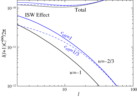
FIG. 2.: ISW effect in the $w=-1$ fiducial model compared with models with $w=-2/3$ and sound speeds $c_{\rm eff}=1,1/3$ with other parameters held fixed. The ISW effect is highly sensitive to the equation of state and clustering properties of the dark energy but only becomes a substantial fraction of the total temperature anisotropy power spectrum at the lowest multipoles.

2 Degeneracies

The Fisher matrix identifies degenerate directions in parameter space through its eigenvectors. It has been intensely studied for primary CMB anisotropies [33, 37] revealing two underlying and related degeneracies. The first is the so-called angular diameter distance degeneracy. A change in parameters that leaves the angular diameter distance to the last scattering surface at recombination and the physics of acoustic oscillations unchanged preserves the structure and locations of the acoustic peaks. In the present context, shifts to lower $l$ by an increase in $w$ can be compensated by a decrease in $\Omega_{\Lambda}$ as long as the physical baryon and matter density are held fixed. The only way to break this degeneracy through the temperature spectrum is to study the ISW contributions at the lowest $l$’s.

The large-scale nature of the ISW effect is both a blessing and a curse. It offers the rare opportunity to study the properties of the dark energy including its clustering (see Fig. 2). However precision in these studies is severely limited by sample variance. Even an all sky experiment has only a handful of realizations of the large scale modes. Worse still, as we shall see next, there are a multitude of effects that can change the spectrum at the lowest $l$’s. The angular diameter distance can be broken in two general ways: with precision measures of a complementary combination of the parameters or through isolation of the ISW effect. The primary example of the former is external constraints on the Hubble constant. In the context of flat cosmologies, the CMB measurement of $\Omega_{m}h^{2}$ combined with $h$-constraints yields a measure of $\Omega_{\Lambda}=1-\Omega_{m}$.

Because of the ISW effect, the angular diameter distance degeneracy is linked with a degeneracy in the amplitude of the peaks relative to the lowest $l$’s. The effect of reionization through $\tau$ is to uniformly lower the amplitude of the peaks compared with the lowest $l$’s since scattering destroys anisotropies. It can therefore be compensated by a change in the initial amplitude $\delta_{\zeta}$ again except for the lowest $l$’s. Finally the tensor contribution also appears only at the lowest $l$’s. To resolve this degeneracy, the effects of reionization, initial amplitude, dark energy and tensors must be separated. Of these only reionization is likely to have direct external constraints, e.g. in the form of a detection of the Gunn-Peterson effect.

In Fig. 1 we show an example that employs both the angular diameter distance degeneracy and the peak amplitude degeneracy. The dashed line represents a model with the parameters: $\Omega_{b}h^{2}=$ same, $\Omega_{m}h^{2}=$ same, $\Omega_{\Lambda}=0.54$, $w=-0.63$, $\tau=0$, $\delta_{\zeta}=4.56\times 10^{-5}$, $T/S=0.015$. From the unlensed temperature power spectrum it is distinguished at only the $0.2\sigma$ level by the Planck experiment which is essentially ideal for these purposes.

B CMB Polarization

The Stokes parameter polarization fields for the linear polarization of the CMB form a tensor field on the sky $T_{1}=U(\hat{\bf n})$, $T_{2}=V(\hat{\bf n})=0$, and $T_{3}=Q(\hat{\bf n})$. We define the corresponding multipole moments in Eqn. (18) as $E_{lm}$ and $B_{lm}$ for $E$ and $B$ modes respectively. Their power spectra and cross-correlation with the temperature field are calculated in the same way as for the temperature anisotropies themselves. The effective noise power of an experiment is given by

$$(N_{l}^{EE})^{-2} = \sum_{i=1}^{N_{\rm chan}}\left[\left({\Delta P\over T}\right)_{i}\sigma_{i}e^{l(l+1)\sigma_{i}/16\ln 2}\right]^{-2}$$ (32)

$$= (N_{l}^{BB})^{-2}\,.$$ (33)

We assume $N_{l}^{\Theta E}=0$. Values for various experiments are given in Tab. I.

As is well known, CMB polarization can break the peak amplitude degeneracy and so also assist in breaking the angular diameter distance degeneracy. Mainly, rescattering during reionization generates a the low $l$ bump in the polarization $E$-power and $\Theta E$ cross spectra (see Fig. 1). Gravitational lensing and tensor fluctuations also generate $B$-mode polarization which can help determine the initial amplitudes of the scalar and tensor fluctuations. The main concern in this route to breaking parameter degeneracies is that the interesting signatures are at the lowest $l$’s where the polarization is at the level of tenths of a $\mu$K and below. The assumption that foreground contamination is negligible compared with the sample errors on the fields themselves is unlikely to hold true [32]. Note that in the context of constraints on the tensor amplitude the gravitational lensing $B$-modes act as a foreground. As we shall see in §IV B, they place a lower limit on the detection threshold for tensors even in the absence of true foregrounds.

C Lensing

The observables of weak lensing of the CMB and faint galaxies are all based on the projected potential $\phi_{i}(\hat{\bf n})$, a scalar field on the sky. It follows the general prescription of a tracer field in §II C with the lensing weight

$$W^{\phi_{i}}(D)={2\over D}\int_{D}^{D(z_{i})}dD^{\prime}{(D^{\prime}-D)\over D^{\prime}}g_{i}(D^{\prime})\,,$$ (34)

from which one can calculate the multipole moments of $\phi_{i}$ and its cross-correlation with other fields. Here $g_{i}(D)$ is the source distribution for the $i$th set of lensed objects.

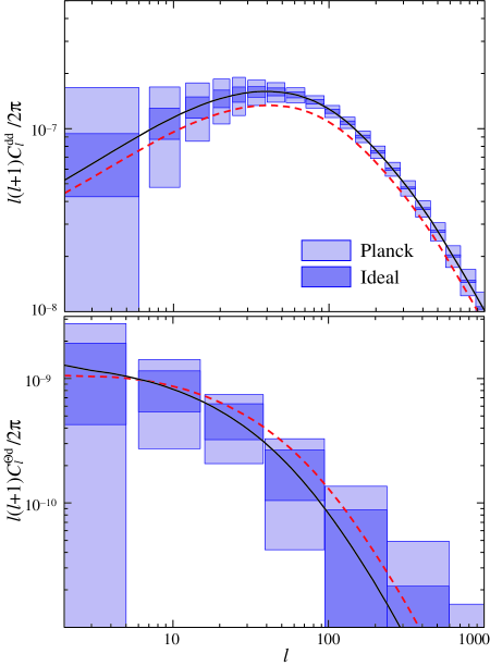
FIG. 3.: CMB lensing power spectra for the fiducial $w=-1$ model (solid) and the degenerate $w=-2/3$ model (dashed) of Fig. 1. Boxes represent 1$\sigma$ errors on band powers assuming the Planck and ideal experiments of Tab. I. Top: deflection power spectra. Bottom: cross correlation of deflection and temperature fields.

1 CMB Lensing

For the CMB, it is the primary anisotropies themselves that are lensed and the source distribution in Eqn. (34) is the Thomson visibility

$$g_{\rm CMB}(D)=\dot{\tau}e^{-\tau(D)}\,,$$ (35)

where here and here only $\tau(D)$ refers to the optical depth out to a distance $D$ and not the reionization optical depth. It may be replaced by a delta function at the last scattering surface $z\sim 10^{3}$.

The associated observable is the deflection angle

$${\bf d}(\hat{\bf n})=\nabla\phi_{\rm CMB}(\hat{\bf n})\,,$$ (36)

which remaps the original temperature field $\tilde{\Theta}$ as $\Theta(\hat{\bf n})=\tilde{\Theta}(\hat{\bf n}+{\bf d})$ and similarly for the polarization field. Its harmonic moments are thus curl free and obey

$$[{d_{1}\pm id_{2}}](\hat{\bf n}) = \pm i\sum_{lm}d_{lm}{}_{\pm 1}Y_{l}^{m}(\hat{\bf n})\,,$$ (37)

$$d_{lm} = -i\sqrt{l(l+1)}\phi_{lm}\,.$$ (38)

These deflections alter the power spectrum of the temperature and polarization fields. On the scales of the acoustic peaks, the main effect is a smoothing of features in the power spectra [26] and the generation of $B$-mode polarization [27]. These are potentially observable and can themselves break parameter degeneracies [28, 29]. One must be careful in that features can also be smoothed and $B$-modes generated artificially by sky cuts and uneven sampling [30].

The deflections also introduce non-Gaussianity into the CMB fields. A negative impact of the non-Gaussianity is that creates a covariance between the power spectra at different $l$’s and technically invalidates the expression for the Fisher matrix (27). The covariance is small and does not affect the bulk of parameter estimation [6]. However it can lead to misleadingly optimistic estimates of parameter forecasts when strong degeneracies like those discussed above are involved (see §IV).

Fortunately, the non-Gaussianity also makes the deflection field itself and its power spectrum $C_{l}^{dd}$ directly observable with quadratic combinations of the temperature field. A quadratic estimator of the deflection field with the optimal noise power spectrum

$$N_{l}^{dd} = \left[\sum_{l_{1}l_{2}}{(C_{l_{2}}^{\tilde{\Theta}\tilde{\Theta}}F_{l_{1}ll_{2}}+C_{l_{1}}^{\tilde{\Theta}\tilde{\Theta}}F_{l_{2}ll_{1}})^{2}\over 2(C_{l_{1}}^{\Theta\Theta}+N_{l_{1}}^{\Theta\Theta})(C_{l_{2}}^{\Theta\Theta}+N_{l_{2}}^{\Theta\Theta})}\right]^{-1}$$ (40)

$$\times l(l+1)(2l+1)\,,$$

was given in [6] and involves the divergence of the temperature weighted temperature-gradient field. Here $\tilde{C}_{l}^{\Theta\Theta}$ is the unlensed CMB spectrum and

$$F_{l_{1}ll_{2}} = \sqrt{(2l_{1}+1)(2l+1)(2l_{2}+1)\over 4\pi}\left(\begin{array}[]{ccc}\!l_{1}\!&l\!&l_{2}\!\\ \!0\!&0\!&0\!\end{array}\right)$$ (44)

$$\times{1\over 2}[l(l+1)+l_{2}(l_{2}+1)-l_{1}(l_{1}+1)]\,.$$

and is approximately Gaussian. The deflection power spectrum for the fiducial model is shown in Fig. 3 (top) along with the degenerate model from Fig. 1 and the band power errors calculated according to the noise spectrum of Eqn. (40). Since the deflection strength depends on the absolute amplitude of the underlying potential, its power spectrum breaks the amplitude degeneracy of the CMB temperature fluctuations. It also probes the dark energy dependent growth rates and distances.

Because the deflections trace the gravitational potential, they are correlated with temperature anisotropies themselves through the ISW effect [34, 35, 36]. The cross-power spectrum is shown in Fig. 3 (bottom). It helps isolate the ISW contribution in the temperature anisotropies and provide a means of constraining the clustering properties of the dark energy as we shall see in §IV D.

Lensing Survey Specifications Experiment area $N_{z}$ $\bar{n}_{i}$ $W_{25}$ 25 1 56 $Z_{25}$ 25 3 (28,14,14) $W_{1000}$ 1000 1 56 $Z_{1000}$ 1000 3 (28,14,14) $W_{65\%}$ 27000 1 56 $Z_{65\%}$ 27000 3 (28,14,14)

TABLE II.: Lensing survey specifications. Area is in deg², source density in gal/arcmin² and median redshift $z=1$ corresponding to band divisions $z<1$, $1<z<1.5$ and $z>1.5$.

2 Cosmic Shear

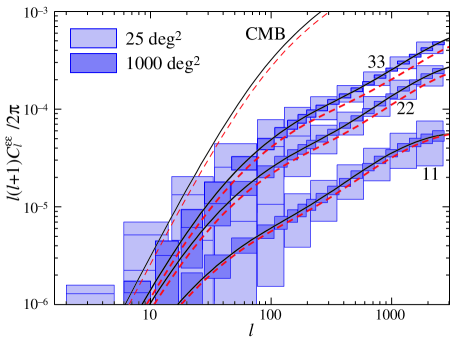
FIG. 4.: Shear power spectra for three redshift bands $z<1$, $1<z<1.5$ and $z>1.5$ for the fiducial model (solid) and the degenerate $w=-2/3$ model of Fig. 1. Error boxes represent $1\sigma$ errors on band powers appropriate to the survey parameters of Tab. II, $Z_{25}$ and $Z_{1000}$.

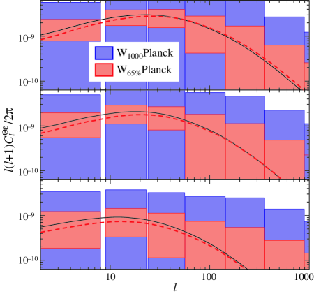
FIG. 5.: Cross correlation of cosmic shear with the CMB temperature in three redshift bands for the fiducial model (solid) and the degenerate $w=-2/3$ model of Fig. 1. Errors are appropriate for Planck and lensing surveys with $1000$ deg² and all of the $65\%$ of sky covered by Planck.

For galaxy weak lensing the distance distribution of the sources is directly related to the source galaxy redshift distribution,

$$g_{i}(D)=n_{i}(z){dz\over dD}\,,$$ (45)

where $n_{i}(z)$ is the normalized redshift distribution $\int dzn_{i}(z)=1$. $n_{i}(z)$ is itself an observable that is produced in conjunction with the survey but for definiteness we take the redshift distribution corresponding to

$$g_{\rm tot}(D)\propto D\exp[-(D/D_{*})^{4}]\,,$$ (46)

with $D_{*}$ fixed by the median redshift taken to be $z=1$. This distribution roughly approximates a survey with a magnitude limit of $R<25$. For cosmic shear, the associated observable is the symmetric trace free shear tensor

$$-[\nabla_{i}\nabla_{j}-{1\over 2}g_{ij}\nabla^{2}]\phi(\hat{\bf n})=[\gamma_{1}(\hat{\bf n})\sigma_{3}+\gamma_{2}(\hat{\bf n})\sigma_{1}]_{ij}\,,$$ (47)

where $g_{ij}$ is the metric on the sphere. Its harmonic moments are magnetic-mode free and obey

$$[{\gamma_{1}\pm i\gamma_{2}}](\hat{\bf n}) = \sum_{lm}\epsilon_{lm}\,{}_{\pm 2}Y_{l}^{m}(\hat{\bf n})\,,$$ (48)

$$\epsilon_{lm} = -{1\over 2}\sqrt{(l+2)!\over(l-2)!}\phi_{lm}\,.$$ (49)

Shot noise produces the noise power spectrum [22]

$$N_{l}^{\epsilon\epsilon}=\langle\gamma_{\rm int}^{2}\rangle/\bar{n}_{i}$$ (50)

where $\langle\gamma_{\rm int}^{2}\rangle^{1/2}$ is the rms intrinsic shear per galaxy due to intrinsic ellipticities and measurement errors. We assume $\langle\gamma_{\rm int}^{2}\rangle^{1/2}=0.4$ throughout. $\bar{n}_{i}$ is the number of galaxies per steradian in the measurement.

With measurements of not just the redshift distribution but of individual source galaxies, the total distribution can be broken into redshift bands to yield separate but correlated power spectra. The evolution of the spectra can be used to probe structures and their evolution tomographically. To test the efficacy of tomography, we divide the total into $N_{z}=3$ redshift bins that contain a fixed fraction of the galaxies (1) the lower half, (2) the third quartile and (3) the upper quartile and label the distributions and as $g_{1}$, $g_{2}$ and $g_{3}$ respectively. The shear power spectra and cross correlation in bands then follow from the prescriptions above. This scheme was found in [11] to be a good trade off between shot noise and signal. Table II lists the parameters of the fiducial surveys used in the Fisher analysis.

Similar to the CMB lensing case, the cosmic shear is correlated with the CMB temperature through the ISW effect as shown in Fig. 5. Because the ISW effect is confined to low-$l$’s, this correlation only becomes measurable with lensing surveys that cover a significant fraction of the sky. Finally the cosmic shear in the higher redshift bands and CMB deflection angles are substantially correlated as shown in Fig. 6. The CMB can thus provide the high redshift anchor for tomography studies.

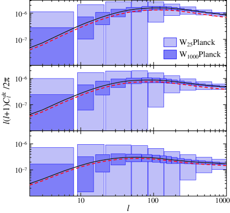
FIG. 6.: Cross correlation of CMB deflection angle with cosmic shear in three redshift bands and errors appropriate for Planck and lensing surveys with $25$ and $1000$ deg².

	$\Omega_{\Lambda}$	$w$	$\tau$	$T/S$	$\ln\delta_{\zeta}$	$n$	$\ln\,\Omega_{m}h^{2}$	$\ln\,\Omega_{b}h^{2}$
T	0.604	1.93	0.1833	0.281	0.1882	0.0746	0.1412	0.0956
TD	0.475	1.42	0.1684	0.263	0.1614	0.0711	0.1334	0.0905
TD4000	0.195	0.53	0.0987	0.142	0.0549	0.0474	0.0719	0.0621
TP	0.330	1.07	0.0267	0.139	0.0448	0.0360	0.0696	0.0493
TPD4000	0.162	0.48	0.0193	0.084	0.0208	0.0185	0.0160	0.0300
TH10	0.083	0.69	0.1714	0.262	0.1832	0.0721	0.1369	0.0937
T$\tau_{10}$	0.565	1.83	0.0050	0.280	0.0834	0.0733	0.1401	0.0947
TW25	0.295	0.87	0.1578	0.110	0.1122	0.0450	0.0745	0.0577
TZ25	0.063	0.29	0.1297	0.094	0.0905	0.0392	0.0660	0.0518
TW1000	0.083	0.19	0.0876	0.077	0.0658	0.0230	0.0435	0.0326
TZ1000	0.010	0.08	0.0522	0.065	0.0426	0.0125	0.0288	0.0222
TPD4000Z1000	0.010	0.04	0.0141	0.060	0.0120	0.0110	0.0102	0.0211

TABLE III.: Fisher parameter estimation errors for MAP and supplemented by various other sources. $T$ refers to temperature spectra, $D$ deflection angles, $P$ polarization, $H$ 10% Hubble constant measurements, $\tau$ 10% optical depth measurements ($\sigma(z_{i})\sim 0.5$), $W$ weak lensing galaxy shear, $Z$ weak lensing galaxy shear with 3 redshift divisions. Experimental assumptions are given in Tab. I and II.

	$\Omega_{\Lambda}$	$w$	$\tau$	$T/S$	$\ln\delta_{\zeta}$	$n$	$\ln\,\Omega_{m}h^{2}$	$\ln\,\Omega_{b}h^{2}$
T	0.581	1.88	0.1724	0.113	0.1715	0.0052	0.0157	0.0084
TD	0.110	0.35	0.0262	0.056	0.0231	0.0051	0.0151	0.0078
TP	0.098	0.32	0.0042	0.007	0.0058	0.0033	0.0094	0.0060
TPD	0.065	0.20	0.0039	0.007	0.0054	0.0030	0.0079	0.0056
TH10	0.070	0.23	0.1641	0.106	0.1635	0.0051	0.0157	0.0082
T$\tau_{10}$	0.553	1.79	0.0050	0.086	0.0086	0.0051	0.0156	0.0082
TW25	0.265	0.86	0.0387	0.057	0.0340	0.0051	0.0152	0.0079
TZ25	0.062	0.20	0.0313	0.054	0.0259	0.0051	0.0152	0.0078
TW1000	0.050	0.15	0.0298	0.053	0.0240	0.0050	0.0148	0.0078
TZ1000	0.010	0.05	0.0258	0.053	0.0208	0.0046	0.0135	0.0076
TPDZ1000	0.010	0.03	0.0036	0.007	0.0039	0.0026	0.0026	0.0045

TABLE IV.: Same as Tab. III but for Planck.

	$\Omega_{\Lambda}$	$w$	$\tau$	$T/S$	$\ln\delta_{\zeta}$	$n$	$\ln\,\Omega_{m}h^{2}$	$\ln\,\Omega_{b}h^{2}$
T	0.451	1.45	0.1343	0.090	0.1335	0.0017	0.0020	0.0012
TD	0.050	0.16	0.0077	0.041	0.0079	0.0016	0.0020	0.0011
TP	0.049	0.16	0.0015	0.000	0.0018	0.0009	0.0008	0.0004
TPD	0.018	0.06	0.0015	0.000	0.0017	0.0009	0.0008	0.0004
TH10	0.069	0.22	0.1299	0.084	0.1292	0.0016	0.0020	0.0011
T$\tau_{10}$	0.435	1.40	0.0050	0.065	0.0054	0.0016	0.0020	0.0011
TW25	0.248	0.80	0.0248	0.045	0.0245	0.0016	0.0020	0.0011
TZ25	0.062	0.20	0.0129	0.042	0.0130	0.0016	0.0020	0.0011
TW1000	0.047	0.15	0.0059	0.041	0.0059	0.0016	0.0020	0.0011
TZ1000	0.010	0.03	0.0043	0.041	0.0046	0.0016	0.0020	0.0011
TPDZ1000	0.008	0.03	0.0012	0.000	0.0015	0.0009	0.0007	0.0004

TABLE V.: Same as for Tab. III but for an ideal CMB experiment out to $l=3000$.

IV Parameter Forecasts

Here we study parameter forecasts using the Fisher matrix formalism of §II D to combine information from the primary CMB anisotropies and gravitational lensing. We give details of the implementation in §IV A and discuss the effect of lensing on the gravitational wave and reionization detectability in §IV B and dark energy properties in §IV C-IV D.

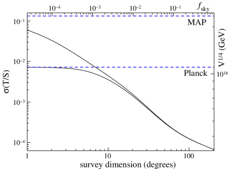
FIG. 7.: Improvement in the polarized MAP and Planck $1\sigma$ detection thresholds for tensors with a dedicated polarization survey. The statistical subtraction of the lensing $B$-mode contamination requires a large survey area and places and ultimate detection threshold of $3-4\times 10^{15}$ GeV for the energy scale of inflation.

A Methodology

The methodology of Fisher-matrix parameter forecasts with the CMB and cosmic shear are well established [33, 37, 11]. Here we simply note the details of our implementation. We approximate the parameter derivatives in the Fisher matrix (27) with finite differences of step size $\Delta\Omega_{b}h^{2}=\pm 0.15\Omega_{b}h^{2}$, $\Delta\Omega_{m}h^{2}=\pm 0.05\Omega_{m}h^{2}$, $\Delta\Omega_{\Lambda}=\pm 0.05\Omega_{m}$, $\Delta n=\pm 0.005n$, $\Delta\delta_{\zeta}=\pm 0.1\delta_{\zeta}$, $\Delta\tau=\pm 0.1\tau$, $\Delta w=0.1w$, $\Delta\log_{10}c_{s}=-2$, where “$\pm$” refers to the fact that two-sided differences are taken for better accuracy. Derivatives with respect to $\delta_{T}$ or $T/S$ are simply proportional to the power spectra themselves since non-linearities never develop in the tensor sector. For the fiducial model of $w=-1$, derivatives with respect to the sound speed vanish identically and consequently these elements are dropped from the Fisher matrix. We truncate the Fisher sum in Eqn. (27) at $l_{\rm max}=3000$; beyond this secondary anisotropies and nonlinearities in the projected potential make the associated CMB and lensing observables non-Gaussian and invalidate the Fisher formalism.

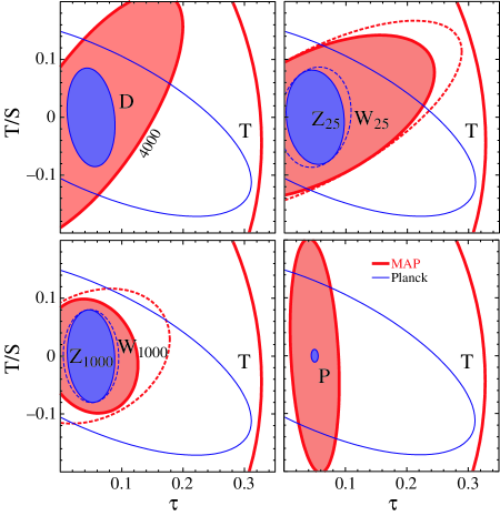
FIG. 8.: Breaking of the tensor-reionization degeneracy. Top-left: addition of CMB deflection angle information (“D”) to the MAP (thick) and Planck (thin) temperature constraints. For MAP, we assume that the deflection angle information comes from a separate $4000$deg² secondary anisotropy survey. For Planck, we assume that they are internal. Top-right: the addition of a $25$ deg² cosmic shear survey with ($Z_{25}$) and without ($W_{25}$) tomographic redshift information. Bottom-left: same but for a $1000$ deg² cosmic shear survey. Bottom-right: addition of polarization information.

As discussed in [37], the angular diameter distance degeneracy must be protected against numerical errors. We replace finite differences in $w$ with those in $\Omega_{\Lambda}$ beyond $l=150$ with the proportionality fixed at this scale. We have tested that the results are insensitive to the exact choice of the matching.

For the CMB power spectra, we have the choice of using the lensed or unlensed power spectra as inputs to the Fisher matrix. As discussed in §III, using the unlensed spectra generally underestimates the information content since lensing breaks parameter degeneracies whereas using the lensed power spectra overestimates the information content due to the non-Gaussian correlation of power spectra errors. One can show that using the lensed power spectra for a ideal experiment out to $l=3000$ and Gaussian assumptions artificially predicts a better breaking of the angular diameter distance degeneracy than complete (cosmic variance limited) information on both the unlensed power spectrum and the deflection angles. The reason is that lensing effects at $l\sim 1000$ still arise from mass structures at $l\sim 100$. Consequently the sample variance on lensing effects is much larger than the Gaussian assumption would imply. For this reason and the fact that we directly measure the deflection spectrum through quadratic statistics, we use the unlensed power spectra in parameter forecasts given in Tab. III-V. The exception is in the discussion of the tensor amplitude and $B$-mode polarization in §IV B. Here the generation of $B$-modes by lensing introduces a foreground to the tensor measurement and the unlensed spectra would give a falsely optimistic limit on the detectability of tensors.

B Tensors and Reionization

Gravitational lensing both provides and obscures information about the tensor or gravitational wave fluctuations. In the absence of lensing and with the complete removal of foregrounds through their frequency dependence, the $B$-mode of the CMB polarization maps provide a direct measure of the tensor contribution that is ultimately limited only by its own cosmic variance. By generating $B$-modes in the polarization with a blackbody spectrum, lensing adds an extra source of noise bias that must be subtracted statistically. Hence the threshold for tensor detectability is set by the sample variance of the lensing not the tensor signal. Without lensing (or foregrounds and systematics) it is always better to go deep on a small patch than shallow on a wide patch. The optimal size is approximately $3^{\circ}\times 3^{\circ}$ [38]. With lensing, more samples of such regions is required to beat down the variance on the lensing contamination if extremely small tensor signals are to be recovered.

To quantify these considerations, we use the Fisher approach to examine the $1\sigma$ threshold for detection of tensors including the lensed polarization as a Gaussian random field. For the detector noise limited, all-sky MAP and Planck missions lensing has essentially no effect on the detectability of tensors.

Lensing does change the optimal strategy for a dedicated polarization experiment that seeks to improve on the Planck experiment as shown in Fig. 7. To reach below $T/S\approx 0.01$ (or inflationary energy scales $<10^{16}$ GeV) and improve on Planck’s potential, a survey area of greater than $10^{\circ}\times 10^{\circ}$ is required.

Note that these considerations assume perfect foreground and systematic error removal (including $E$, $B$-mode separation in a finite survey) as well as a Gaussian $B$-field from lensing. As such, they should be taken as a lower limit on the detectability of tensors. Conversely, they assume statistical subtraction only; limits can be improved if direct subtraction methods can be developed.

Lensing also indirectly assists the detection of tensors in the absence of polarization. Since lensing is sensitive to the absolute amplitude of the potential fluctuations, measurements of the CMB deflection power spectrum or cosmic shear power spectra can break the amplitude degeneracy of the CMB acoustic peaks and so improve the errors on both tensors and the reionization optical depth.

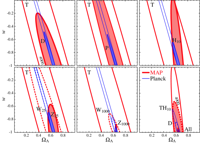
FIG. 9.: Improvement on the MAP (thick) and Planck (thin) temperature ($T$) determination of the dark energy equation of state and density. Clockwise from the top left: addition of CMB deflection angles ($D$); polarization ($P$); 10% Hubble constant measurements ($H$); 25 deg² cosmic shear survey with ($Z$ solid) and without ($W$ dashed) tomography; same but for 1000 deg²; Hubble constant ($TH$), plus deflections ($D$), plus a 1000 deg² lensing survey (All).

In Fig. 8, we quantify this degeneracy breaking. While polarization information still provides better constraints on tensors and reionization, deflection angle information can improve errors on $\tau$ by $2-20$ (MAP to Ideal CMB experiment) and $T/S$ by $2$. Cosmic shear can help by a comparable but somewhat smaller amount with or without tomographic information. The reionization epoch is also potentially directly observable in the Gunn-Peterson effect and so we show the influence of a prior of $\sigma(\tau)=0.1\tau$ on the other parameters in Tab. III-V.

C Equation of State

As is well known and shown in Fig. 9, there is an angular diameter distance degeneracy between the dark energy equation of state $w$ and energy density $\Omega_{\Lambda}$. There are many ways to break the angular diameter distance degeneracy some involving pure geometry and other employing the clustering properties of the dark matter and dark energy. As such strong consistency checks will be available for parameter constraints and underlying assumptions for dark energy parameters.

Although both MAP and Planck show a strong degeneracy, it is important to note that for the Planck experiment the direction orthogonal to the degeneracy line is highly constrained. This corresponds to the better constraints on $\Omega_{m}h^{2}$ which also enters into the angular diameter distance relation.

A purely geometric way of breaking the degeneracy then is to introduce constraints on the Hubble constant. In a flat universe, a precise determination of $\Omega_{m}h^{2}$ combined with constraints on $h$ yield corresponding constraints on $\Omega_{\Lambda}=1-\Omega_{m}$ as shown in Fig. 9. For the Planck experiment, the 10% measurement of the Hubble constant currently claimed [39] is sufficient to yield an interesting constraint on the equation of state $\sigma(w)=0.23$ (see Tab. IV). Using the baryon bumps in the galaxy power spectrum as a standard ruler to measure the Hubble constant, this means of degeneracy breaking can potentially be substantially improved [37].

As seen in Fig. 3, the CMB deflection power spectrum is another means of breaking the degeneracy. It differs by also involving the effect of the dark energy on the clustering of the matter. Because of the nature of the quadratic estimator of the deflection angle, it is crucial here to resolve CMB temperature anisotropies through the damping tail to $l\sim 3000$ [6]. This is reflected in the negligible improvement in $\sigma(w)$ for MAP alone to the order of magnitude improvement for the ideal experiment.

Information on the deflection power spectra do not have to come from the same experiment as that for the temperature anisotropies themselves. To measure deflection angles, one requires high resolution in the temperature map but essentially no information on the large-scale anisotropy itself. Combining an all sky experiment such as MAP with an experiment that is dedicated to measuring secondary arcminute scale anisotropies can therefore be fruitful. We show in Fig. 9 that a $4000$ deg² survey is sufficient to provide interesting constraints on the equation of state.

Similarly cosmic shear power spectra also provide information on the equation of state. As shown by [9], if the whole power spectrum can be recovered to $l=10000$ and theoretical predictions in the deeply non-linear regime improved, a single redshift band suffices to yield powerful constraints on the equation of state in the Gaussian approximation. Non-linearities produce non-Gaussianity in the cosmic shear that degrades the amount of information in the deeply non-linear regime beyond $l\sim 3000$ [40]. In Fig. 9 we show that information in the trans-linear regime of $l<3000$ suffices to determine the dark energy equation of state when broken into multiple redshift bands and combined with CMB temperature information. Notice that redshift information on a 25 deg² survey (filled ellipses) is competitive with no redshift information on a 1000 deg² survey (dashed ellipses).

With the multitude of avenues for constraints on the dark energy equation of state discussed above as well as those from high redshift supernovae [2] and number counts [41], it is possible that the observations will be inconsistent with the simple underlying model of a constant equation of state and dark energy clustering appropriate for a single slowly-rolling scalar field. Since geometric tests can potentially probe the time evolution of the equation of state, we conclude in the next section with a discussion of dark energy clustering.

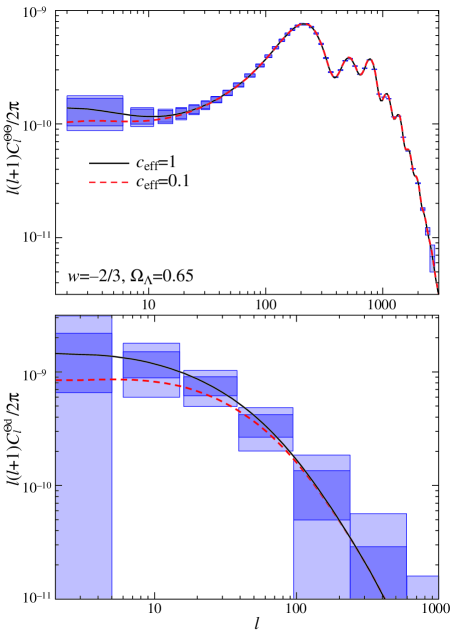
FIG. 10.: Dark energy clustering in a model with $w=-2/3$ and $c_{s}=1$, $0.1$ and other parameters the same as in the fiducial model. Top: effect on the CMB. Bottom: cross correlation of deflection angles with the temperature anisotropies.

	Planck			Ideal
	$\Omega_{\Lambda}$	$w$	$\log_{10}c_{\rm eff}$	$\Omega_{\Lambda}$	$w$	$\log_{10}c_{\rm eff}$
T	0.4377	1.105	4.1221	0.3527	0.890	3.2039
TD	0.0861	0.215	1.0938	0.0329	0.083	0.4973
TP	0.1967	0.497	1.1856	0.1085	0.274	0.8531
TPD	0.0431	0.099	0.7516	0.0088	0.021	0.3828
TH10	0.0693	0.179	3.8768	0.0687	0.173	3.0108
TW25	0.2377	0.599	1.4426	0.2201	0.556	1.1640
TZ25	0.0623	0.158	1.3827	0.0618	0.156	1.0978
TW1000	0.0479	0.114	1.3599	0.0447	0.113	1.0798
TZ1000	0.0106	0.030	1.3497	0.0099	0.025	1.0724
TPDZ1000	0.0098	0.023	0.7264	0.0058	0.014	0.3790

TABLE VI.: Fisher parameter estimation errors for dark energy parameters in a fiducial $w=-2/3$ model. Notation follows Tab. III. Parameters not shown are marginalized.

D Dark Energy Clustering

If the equation of state of the dark energy $w>-1$, then there is a new dimension to the dark energy defined by its clustering properties. In §II A, we introduced the sound speed of the dark energy for this purpose. Recall that the scalar field candidate for the dark energy has $c_{\rm eff}=1$.

As shown in Fig. 2 and 10, the ISW effect in the CMB rapidly decreases with the sound speed but is difficult to isolate from other contributions to the anisotropies at low $l$. By breaking the amplitude degeneracy, the deflection power and cosmic shear power spectra help isolate the ISW effect. Furthermore the deflection angles are themselves correlated with the temperature anisotropies leading to an additional more direct handle on the dark energy clustering (see Fig. 10 bottom). For Planck the constrains are are equivalent to saying the dark energy is smooth at least across $\sim$10% of the current horizon or 1.4 Gpc in the fiducial model. As Tab. VI shows, there is room for substantial improvement especially on the CMB deflection angle side for a next generation mission with higher angular resolution. With an ideal CMB experiment to $l=3000$ and a cosmic shear survey with $1000$deg², the dark energy smoothness an be constrained to be $\sim$40% of the current horizon or 6 Gpc. If cosmic shear surveys can reach the sky coverage and control of systematics to measure the multipoles $l\ll 100$ then additional information and consistency checks will be available from their cross-correlation with the CMB temperature maps (see Fig. 5). Note however that these constraints greatly weaken as the equation of state approaches $-1$.

V Discussion

Gravitational lensing as manifest in CMB deflection and cosmic shear measurements complements CMB primary anisotropies by providing information that breaks degeneracies involving the dark energy density and equation of state, reionization and gravitational waves, specifically the angular diameter distance degeneracy and the amplitude degeneracies in the acoustic peaks. In this way, it is similar in utility to the well-studied CMB polarization and offers sharp consistency checks on the difficult-to-measure dark energy parameters. Conversely, CMB lensing obscures polarization information on the gravitational waves and necessitates large sky coverage to beat down sample variance even with perfect detectors and no foregrounds.

CMB lensing offers information that is similar to cosmic shear but with important additional strengths and weaknesses. Its primary strengths are that it is intrinsically more sensitive to structure on larger scales and higher redshifts than even the next generation of wide-field galaxy surveys. These strengths translate into the opportunity to study the clustering of the dark energy, primarily through cross-correlation with the ISW effect. Indeed any such correlation is a direct indication of dark energy in a spatially flat universe. Its primary disadvantage is that the sources are confined to a single epoch, the last scattering surface, so that tomographic studies of the evolution of the dark energy and dark matter are impossible. Galaxy lensing with source redshift information can therefore better constrain the equation of state of the dark energy including potentially its evolution.

It is important to realize that Fisher parameter forecasts include statistical errors only making the blind combination of information from disparate sources dangerous. In particular, the information supplied by lensing relies in large part on the accurate absolute calibration of the power spectra. On the CMB lensing side, this involves first an accurate determination of the CMB power spectrum itself as well as any detector or foreground power spectrum contaminants. On the cosmic shear side, it requires exquisite control over the myriad systematics that enter into the measurement of shear from galaxy images. Furthermore, Fisher forecasts are only probe the degeneracy structure locally around a fiducial model. When error ellipses are extended in parameter space due to degeneracies, Fisher forecasts can yield both overly optimistic or pessimistic results. Our results provide the motivation for future studies that do incorporate these systematic effects involving the combination of cosmological information from CMB anisotropy and gravitational lensing.

Acknowledgements: I acknowledge useful conversations with R. Caldwell, A.R. Cooray, D.J. Eisenstein, D. Huterer, J. Miralde-Escude, M. Zaldarriaga and the participants of the Aspen Wide-Field Survey workshop where this work was begun. This work was supported by NASA NAG5-10840, DOE OJI and an Alfred P. Sloan Foundation Fellowship.

A Potential Evolution and Transfer Function

Above the sound horizon of the dark energy, defined as

$$s(a)=\int_{z}^{z_{i}}{dz^{\prime}\over H(z^{\prime})}c_{\rm eff}\,,$$ (A1)

where $z_{i}$ is some initial effectively infinite redshift, the Bardeen curvature remains constant after radiation becomes negligible at some epoch $z_{\rm md}$. The Newtonian curvature consequently obeys

$$\Phi(k,z)=\Phi_{c}(z)\zeta(k,z_{\rm md})\,,$$ (A2)

where the decay function in the clustering regime is [42]

$$\Phi_{c}(z)=\left(1-{\sqrt{\rho}\over a}\int_{0}^{a}{da\over\sqrt{\rho}}\right)\,,$$ (A3)

where $a=(1+z)^{-1}$. Conversely, for scales that are much smaller than the sound horizon at the epoch of dark energy domination the dark energy may be considered effectively smooth for all time and hence the Newtonian curvature obeys

$$\Phi(k,z)=\Phi_{s}(k,z)\zeta(k,z_{\rm md})\,,$$ (A4)

where

$$\Phi_{s}^{\prime\prime}+[{5\over 2}-{3\over 2}w\Omega_{\Lambda}(z)]\Phi_{s}^{\prime}+{3\over 2}[1-w]\Omega_{\Lambda}(z)\Phi_{s}=0$$ (A5)

and ^′ denotes derivatives with respect to $\ln a$. To match solutions $\Phi_{c}(z_{\rm md})=\Phi_{s}(z_{\rm md})$ in the matter dominated epoch, the initial conditions are set to be $\Phi_{s}(z_{\rm md})=3/5$, $\Phi_{s}^{\prime}(z_{\rm md})=0$.

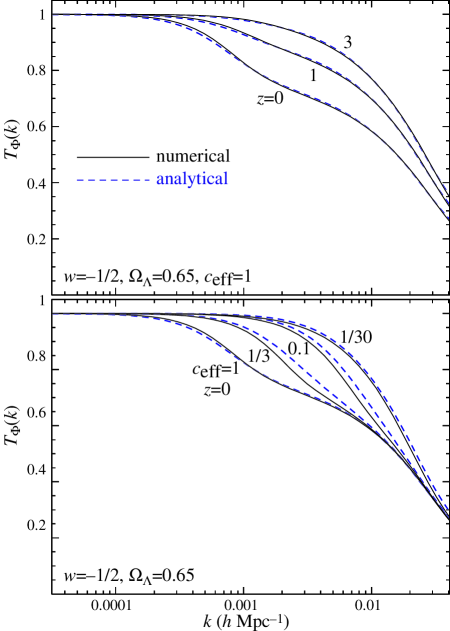
FIG. 11.: Potential transfer function as a function of redshift (top) and dark energy sound speed (bottom). Solid lines represent numerical results; dashed lines represent the analytic fits of [14] supplemented by dark energy clustering.

The decay function in the intermediate regime can be approximated with a smooth interpolation of these two solutions. First we define the epoch of dark energy domination as

$${\rho_{\Lambda}(z_{\Lambda})\over\rho_{m}(z_{\Lambda})}={1\over\pi}\,,\quad(1+z_{\Lambda})=\left(\pi{\Omega_{\Lambda}\over\Omega_{m}}\right)^{-{1\over 3w}}\,,$$ (A6)

where the solution assumes a constant equation of state. Next, we introduce the interpolation function

$$T_{w}(k,z)={{1+q^{2}}\over{\Phi_{s}/\Phi_{c}+q^{2}}}\,,$$ (A7)

where

$$q\equiv{k\over 2\pi}\sqrt{s(z)s(z_{\Lambda})}\,.$$ (A8)

The full evolution of the potential from the matter dominated epoch on can be described by

$$\Phi(k,z)=T_{w}(k,z)\Phi_{s}(z)\zeta(k,z_{\rm md})\,.$$ (A9)

Since in the matter dominated regime, the potential is related to the matter density fluctuations by the Poisson equation, the potential transfer function asymptotically approaches a scaled version of the matter transfer function $T_{m}(k)$ at high $k$

$$T_{\Phi}(k,z) = {\Phi(k,z)\over\Phi(0,z)}{\Phi(0,z_{i})\over\Phi(0,z)}\,.$$ (A10)

$$= {T_{w}(k,z)\over T_{w}(0,z)}T_{m}(k)\,,$$ (A11)

where $T_{m}(k)$ is the matter transfer function assuming scale-independent growth (a smooth dark energy component). Note that the true matter transfer function is still not the same as the potential transfer function due to dark energy contributions to the Poisson equation. Moreover, their is no one unique matter transfer function since it the presence of dark energy clustering the growth of density perturbations differs between the commonly used synchronous and comoving gauges. The Newtonian potential transfer function is most closely related to the comoving gauge matter transfer functions and is in fact the density-weighted sum of the components.

REFERENCES

- [1]
- [2] A.G. Riess, et al. Astron. J, 116 1009 (1998); S. Perlmutter, et al. ApJ, 517 565 (1999).
- [3] A.D. Miller, et al. Astrophys. J Lett., 524 L1 (1999); P. de Bernardis, et al. Nature, 404 955 (2000); S. Hanany, et al. Astrophys. J Lett., 545 5 (2000).
- [4] M. Zaldarriaga, U. Seljak, Phys. Rev. D, 59 123507 (1999).
- [5] M. Zaldarriaga, Phys. Rev. D, 62 063510 (2000).
- [6] W. Hu, Phys. Rev. D, in press (2001, astro-ph/0105117); W. Hu, Astrophys. J Lett., in press (2001, astro-ph/0105424).
- [7] W. Hu, M. Tegmark, Astrophys. J Lett., 514 65 (1999).
- [8] W. Hu, D.J. Eisenstein, M. Tegmark, M. White, Phys. Rev. D, 59 023512 (1999).
- [9] D. Huterer, Astrophys. J, submitted 2001 (astro-ph/0106399).
- [10] M. White, W. Hu, Astrophys. J, 537 1 (2000).
- [11] W. Hu, Astrophys. J Lett., 522 21 (1999).
- [12] J.M. Bardeen, Phys. Rev. D, 22 1882 (1980).
- [13] A.R. Liddle, D.H. Lyth, Phys. Rept., 231 1 (1993).
- [14] D.J. Eisenstein, W. Hu, Astrophys. J, 511 5 (1999).
- [15] C.P. Ma, R.R. Caldwell, P. Bode, L. Wang, Astrophys. J, 521 L1 (1999).
- [16] J.A. Peacock, S.J. Dodds, Mon. Not. Roy. Astr. Soc., 280 19 (1996). This prescription works equally well in dark energy models (M. White private communication).
- [17] W. Hu, M. White, Phys. Rev. D, 56 596 (1997).
- [18] W. Hu, Astrophys. J, 506 485 (1998).
- [19] J. Frieman, C. Hill, A. Stebbins, I. Waga, Phys. Rev. Lett., 75 2077 (1995);; B. Ratra & P. J. E. Peebles, Phys. Rev. D. 37, 3406 (1988); R. R. Caldwell, R. Dave, & P. J. Steinhardt, Phys. Rev. Lett. 80 1582 (1998).
- [20] A.E. Schulz, M. White, Phys. Rev. Lett., submitted (2001, astro-ph/0104112).
- [21] E. Newman, R. Penrose, J. Math Phys. 7, 863 (1966); J.N. Goldberg et al., ibid, 8, 2155 (1967).
- [22] N. Kaiser, Astrophys. J, 388 272 (1992).
- [23] U. Seljak, M. Zaldarriaga, Astrophys. J, 469 437 (1996).
- [24] M. Tegmark, A. Taylor, A. Heavens, Astrophys. J, 480 22 (1997).
- [25] M. White, D. Scott, Astrophys. J, 459 415 (1996).
- [26] U. Seljak, Astrophys. J, 463 1 (1996).
- [27] M. Zaldarriaga, U. Seljak, Phys. Rev. D, 58 023003 (1998).
- [28] R.B. Metcalf, J. Silk, Astrophys. J, 489 1 (1997).
- [29] R. Stompor, G. Efstathiou, Mon. Not. Roy. Astr. Soc., 302 735 (1999).
- [30] M. Tegmark, A. de Oliveira-Costa, PRD, submitted (2001, astro-ph/0012120).
- [31] W. Hu, Phys. Rev. D, 62 043007 (2000).
- [32] M. Tegmark, D.J. Eisenstein, W. Hu, A. de Oliviera Costa, Astrophys. J, 530 133 (2000).
- [33] G. Jungman, M. Kamionkowski, A. Kosowsky, D.N. Spergel, Phys. Rev. D, 54 1332 (1995); M. Zaldarriaga, D.N. Spergel, U. Seljak, Astrophys. J, 488 1 (1997); J.R. Bond, G. Efstathiou, M. Tegmark, Mon. Not. Roy. Astr. Soc., 291 L33 (1997).
- [34] U. Seljak, M. Zaldarriaga, Phys. Rev. D, 60 043504 (1999).
- [35] D.M. Goldberg, D.N. Spergel, Phys. Rev. D, 59 103002 (1999).
- [36] A.R. Cooray, W. Hu, Astrophys. J, 534 533 (2000).
- [37] D.J. Eisenstein, W. Hu, M. Tegmark, Astrophys. J, 518 2 (1999).
- [38] A.H. Jaffe, M. Kamionkowski, L. Wang, Phys. Rev. D, 61 083501 (2000).
- [39] W.L. Freedman, et al. Astrophys. J, 553 47 (2001).
- [40] A.R. Cooray, W. Hu, Astrophys. J, in press 2001 (astro-ph/0012087).
- [41] Z. Haiman, J.J. Mohr, G.P. Holder, Astrophys. J, 553 545 (2001).
- [42] W. Hu, D.J. Eisenstein, Phys. Rev. D, 52 083509 (1999).