ANNz: estimating photometric redshifts using artificial neural networks

Abstract

We introduce annz, a freely available software package for photometric redshift estimation using Artificial Neural Networks. annz learns the relation between photometry and redshift from an appropriate training set of galaxies for which the redshift is already known. Where a large and representative training set is available annz is a highly competitive tool when compared with traditional template-fitting methods.

The annz package is demonstrated on the Sloan Digital Sky Survey Data Release 1, and for this particular data set the r.m.s. redshift error in the range $0\lesssim{z}\lesssim{0.7}$ is $\sigma_{\mathrm{rms}}=0.023$. Non-ideal conditions (spectroscopic sets which are small, or which are brighter than the photometric set for which redshifts are required) are simulated and the impact on the photometric redshift accuracy assessed.

The package may be freely downloaded from http://www.ast.cam.ac.uk/~aac.

1. Introduction

In its most general sense, the term photometric redshift refers to a redshift estimated using only medium- or broad-band photometry or imaging. Most commonly, photometric redshifts are determined on the basis of galaxies’ colours in three or more filters (thus giving a very coarse approximation to the spectral energy distribution, hereafter SED), but they could also be based on other properties which can be derived from images, such as the angular size or concentration index. The method has found successful application to deep-field and wide-field surveys, notably the Hubble Deep Field (e.g. Fernández-Soto, Lanzetta, & Yahil, 1999), and the Sloan Digital Sky Survey (Csabai et al., 2003).

The most commonly used approach to photometric redshift estimation is the template-matching technique. This requires a set of ‘template’ SEDs covering a range of galaxy types, luminosities and redshifts appropriate to the population for which photometric redshifts are required. For a particular target galaxy, the photometric redshift is chosen to be the redshift of the most closely matching template spectrum; this is usually defined as the template which minimizes the $\chi^{2}$ between the template and actual magnitudes.

The template spectra are usually derived from a small set of SEDs representing different classes of galaxy at redshift $z=0$, which are then manually redshifted to give a discrete sampling along the redshift axis (note that this method does not account for evolution with redshift). Commonly used template sets are the Coleman, Wu, & Weedman (CWW; 1980) SEDs which are derived observationally, or those of Bruzual & Charlot (1993), derived from population synthesis models. The template-matching technique owes its popularity to the very few resources required for a basic implementation (i.e. a handful of template SEDs), but the accuracy of the technique strongly depends on the extent to which the template spectra are representative of the target populations: for example, template SEDs derived from observations of low-redshift galaxy populations may be a poor match for populations at higher redshifts.

The chances of success can be improved by increasing the number of templates, or by more carefully matching the templates to the populations being studied. For example, the spectroscopic catalogue of the Sloan Digital Sky Survey (SDSS; York et al. 2000) could be used to produce a set of templates which are very well representative of the SDSS photometric catalogue (Csabai et al., 2003). However, in situations with such a large amount of prior redshift information about the sample, the template-matching technique is not the best approach: so-called empirical methods usually offer greater accuracy, as well as being far more efficient.

In essence, empirical photometric redshift methods aim to derive a parametrization for the redshift as a function of the photometric parameters. The form of this parametrization is deduced through use of a suitably large and representative training set of galaxies for which we have both photometry and a precisely known redshift. A simple example is to express the redshift as a polynomial in the galaxy colours (e.g. Connolly et al. 1995; Sowards-Emmerd et al. 2000). The coefficients in the polynomial are varied to optimize the fit between the predicted and measured redshift. The photometric redshift for the galaxies for which we have no spectroscopy can then be estimated by applying the optimized function to the colours of the target galaxy.

Ideally the training set would be a representative subset of the actual photometric target sample (this has the attractive side-effect of nullifying any systematics in the photometry). However, the training set could also be derived from a set of template spectra or from simulated catalogues (e.g. Vanzella et al. 2003). The photometry for the training set must be for the same filter set and should have the same noise characteristics as that for the target sample. The trained method can usually only be reliably applied to target galaxies within the ranges of redshift and spectral type adequately sampled by the training set.

In this paper we introduce annz, a software package for photometric redshift estimation using Artificial Neural Networks (hereafter ANNs) to parametrize the redshift-photometry relation. It can be shown (e.g. Jones 1990; Blum & Li 1991) that a sufficiently complex ANN is capable of approximating to arbitrary accuracy any continuous functional mapping. ANNs have previously found a number of applications in astronomy, including morphological classification of galaxies (e.g. Lahav et al. 1996; Ball et al. 2003) star/galaxy separation (Bertin & Arnouts, 1996) and object detection (e.g. Andreon et al., 2000). Firth, Lahav, & Somerville (2003) previously demonstrated the feasibility of using ANNs for photometric redshift estimation, and more recently Vanzella et al. (2003) have applied the method to the Hubble Deep Fields.

The layout of this paper is as follows. In §2 Artificial Neural Networks are introduced, and the particular methods used by annz are explained. In §3 annz is applied to the Sloan Digital Sky Survey. The results are compared with rival photometric redshift estimators and various extensions to the basic technique are explained and illustrated. Finally, less ideal conditions are simulated to assess the impact on the accuracy of photometric redshift estimation. In §4 the results are summarised, and prospects for the application of annz discussed.

2. Artificial neural networks

annz uses a particular species of ANN known formally as a multi-layer perceptron (MLP). A MLP consists of a number of layers of nodes (Fig. 1; see e.g. Bishop 1995, and references therein, for background). The first layer contains the inputs, which in our application to photometric redshift estimation are the magnitudes, $m_{i}$, of a galaxy in a number of filters (for ease of notation we arrange these in a vector $\mathbf{m}\equiv(m_{1},m_{2},...,m_{n})$). The final layer contains the outputs; we will usually use just one output, the photometric redshift $z_{\mathrm{phot}}$, but see §3.2.2 for an example with multiple outputs. Intervening layers are described as hidden and there is complete freedom over the number and size of hidden layers used. The nodes in a given layer are connected to all the nodes in adjacent layers. A particular network architecture may be denoted by $N_{\mathrm{in}}$:$N_{1}$:$N_{2}$: $\ldots$ :$N_{\mathrm{out}}$ where $N_{\mathrm{in}}$ is the number of input nodes, $N_{1}$ is the number of nodes in the first hidden layer, and so on. For example 9:6:1 takes 9 inputs, has 6 nodes in a single hidden layer and gives a single output.

Figure 1.— A schematic diagram of a multi-layer perceptron, as implemented by annz, with input nodes taking, for example, magnitudes $m_{i}=-2.5\log_{10}f_{i}$ in various filters, a single hidden layer, and a single output node giving, for example, redshift $z$. The architecture is $n$:$p$:1 in the notation used in this paper. Each connecting line carries a weight $w_{ij}$. The bias node allows for an additive constant in the network function defined at each node. More complex networks can have additional hidden layers and/or outputs.

Each connection carries a weight, $w_{ij}$; these comprise the vector of coefficients, $\mathbf{w}$, which are to be optimized. An activation function, $g_{j}(u_{j})$, is defined at each node, taking as its argument

$$u_{j}=\sum_{i}w_{ij}g_{i}(u_{i}),$$ (1)

where the sum is over all nodes $i$ sending connections to node $j$. The activation functions are typically taken (in analogy to biological neurons) to be sigmoid functions such as $g_{j}(u_{j})=1/[1+\exp{(-u_{j})}]$, and we follow this approach here. An extra input node – the bias node – is automatically included to allow for additive constants in these functions.

For a particular input vector, the output vector of the network is determined by progressing sequentially through the network layers, from inputs to outputs, calculating the activation of each node (hence this type of neural network is often referred to as a feed-forward network).

2.1. Network training

Given a suitable training set of galaxies for which we have both photometry, $\mathbf{m}$, and a spectroscopic redshift, $z_{\mathrm{spec}}$, the ANN is trained by minimizing the cost function

$$E=\sum_{k}(z_{\mathrm{phot}}(\mathbf{w},\mathbf{m}_{k})-z_{\mathrm{spec},k})^{2},$$ (2)

with respect to the weights, $\mathbf{w}$, where $z_{\mathrm{phot}}(\mathbf{w},\mathbf{m}_{k})$ is the network output for the given input and weight vectors, and the sum is over the galaxies in the training set. To ensure that the weights are regularized (i.e. that they do not become too large), an extra quadratic cost term

$$E_{\mathrm{w}}=\beta\sum_{i,j}w_{ij}^{2},$$ (3)

is added to equation 2.

annz uses an iterative quasi-Newton method to perform this minimization. Details of the minimization algorithm and regularization may be found in Bishop (1995) and Lahav et al. (1996, Appendices).

After each training iteration, the cost function is also evaluated on a separate validation set. After a chosen number of training iterations, training terminates and the final weights chosen for the ANN are those from the iteration at which the cost function is minimal on the validation set. This is useful to avoid over-fitting to the training set if the training set is small. The trained network may then be presented with previously unseen input vectors, and the outputs computed.

2.2. Photometric noise

In real situations the inputs to the network (e.g. the magnitudes in this case of photometric redshift estimation) will usually have a measurement noise associated with them. We can assess the variance these errors effect in the output using the usual chain-rule approach:

$$\sigma_{z}^{2}=\sum_{i}{\Big{(}\frac{\partial{z}}{\partial{m_{i}}}\Big{)}^{2}\sigma_{m_{i}}^{2}},$$ (4)

where the sum is over the network inputs.

Given a trained network, the output is an analytic function of the network weights and the input vector: $z=z(\mathbf{w},\mathbf{m})$. Provided the activation functions, $g_{i}(u_{i})$, are differentiable, the derivatives $\partial{z}/\partial{m_{i}}$ can be obtained through a simple and efficient algorithm (Bishop, 1995, pp.148–150). This method is used by annz to estimate the variance in its photometric redshifts due to the photometric noise.

2.3. Network variance

Prior to training, annz randomizes the initial values of the weights. Depending on the particular initialization state used, the training process will usually converge to different local minima of the cost function. A simple possibility is to train a number of networks and select one based on the best performance on the validation set. However, this is wasteful of training effort and, in fact, the sub-optimal networks can be used to improve overall accuracy: the mean of the individual outputs of a group of networks (known as a committee) will usually be a more accurate estimate for the true redshift than the outputs of any one committee member in isolation.

Using a committee also allows the uncertainty in the output due to the variance in the network weights to be estimated. For a particular target galaxy the photometric redshift prediction should ideally be robust to different intializations of the weight vector. However, it may be the case that the available photometry or training set does not constrain the redshift very well (even for high signal-to-noise photometry, so the error estimated by the method of §2.2 could be relatively small). These cases are more likely to show a large variance in the output for different initializations of the weight vector, hence using a committee may assist in their identification. annz allows arbitrarily large committees to be used, and estimates the contribution of the network variance to the error in the photometric redshift for each target galaxy.

2.4. Using the ANNz package

We have made annz available on the WWW at the following address: http://www.ast.cam.ac.uk/~aac. Full instructions are provided with the package, but we provide an outline of the procedure here. annz comprises two main programs, annz_train and annz_test.

1

When applying annz to any data set for the first time it is strongly recommended that a portion of the available training data be set aside as an evaluation set. This is used as a mock target sample to assess and tune annz’s performance on the data. The evaluation set should therefore be chosen to match the real target sample as closely as possible in terms of its magnitude and colour distributions.

2

The remaining training data should be separated into training and validation sets which are supplied to the annz_train program along with a description of the required network architecture. This program performs the network training as described in §2.1. The trained network weights are saved to file.

3

Step 2 may be repeated several times using different network initialisations to obtain a committee of trained networks.

4

The annz_test program can now be used to apply the trained networks to the target data.

Before applying annz to the actual photometric target sample, the whole procedure should be run several times using the evaluation set as the target data, and varying the parameters of the training (e.g. weight decay, training and validation set sizes, number of networks in the committee) so as to optimize the performance.

3. Application to SDSS data

The Sloan Digital Sky Survey (SDSS; York et al. 2000) combines a large, five-band ($ugriz$) imaging survey with a smaller spectroscopic follow-up survey. This is an ideal situation for the application of annz since the spectroscopic survey represents an excellent training set for the imaging survey.

The selection algorithm for the SDSS spectroscopic survey results in two subsets of the data: a main galaxy catalogue and a luminous red galaxy catalogue (LRG; Eisenstein et al., 2001). The main galaxy catalogue is a flux-limited sample ($r<17.77$) with a median redshift $z=0.104$ (Strauss et al., 2002), while the LRG catalogue is flux- and colour-selected to be a very uniform and approximately volume-limited sample (it is volume limited to $z\approx 0.4$, but probes out to $z\approx 0.6$ at lower completion).

3.1. Comparison of ANNz with other techniques

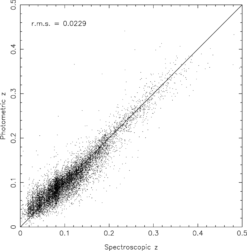
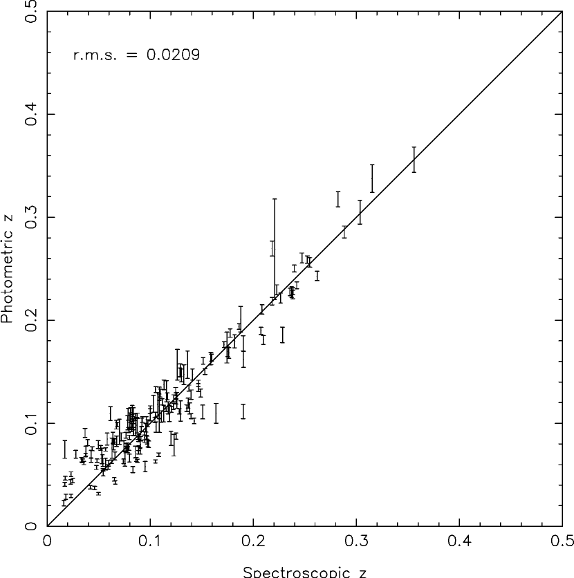
The SDSS consortium have themselves applied a range of photometric redshift techniques to their commissioning data (Csabai et al., 2003). Table 1 lists the estimation errors they obtained. This commissioning data was made public in the Early Data Release (EDR; Stoughton et al., 2002). In order to allow a direct comparison of the accuracy of annz with the methods used by Csabai et al. (2003) we selected the main galaxy and LRG samples from the EDR. From these $\sim$30,000 galaxies we randomly selected training, validation and evaluation sets with respective sizes 15,000, 5,000 and 10,000. The network inputs were the dereddened model magnitudes in each of the five filters and the overall architecture was 5:10:10:1. A committee of five such networks was trained on the training and validation sets, then applied to the evaluation set. Figure 2 shows the annz photometric redshift against the spectroscopic value for each galaxy in the evaluation set. The rms deviation between these is $\sigma_{\mathrm{rms}}=\sqrt{\langle{}(z_{\mathrm{phot}}-z_{\mathrm{spec}})^{2}\rangle{}}=0.0229$, which compares well with the results in Table 1. For clarity the estimated errors on the photometric redshifts are not shown in Fig. 2. The results for a randomly-selected subset of 200 galaxies are shown with errorbars in Figure 3. Due to the high quality of the training data in this case, network variance makes only a small contribution and the errors are therefore dominated by the photometric noise.

Figure 2.— Spectroscopic vs. photometric redshifts for annz applied to 10,000 galaxies randomly selected from the SDSS EDR.

Figure 3.— A subset of 200 galaxies randomly selected from the results of Fig. 2, and with the error bars calculated by annz shown. These are a combination of contributions from photometric noise (§2.2) and network variance (§2.3).

Table 1Photometric redshift accuracies for the SDSS EDR

Estimation Method	$\sigma_{\mathrm{rms}}$
CWW	0.0666
Bruzual-Charlot	0.0552
Interpolated	0.0451
Polynomial	0.0318
Kd-tree	0.0254
annz	0.0229

Note. — The first five entries are the photometric redshift accuracies obtained by Csabai et al. (2003) for the SDSS Early Data Release. The result obtained using annz is appended for comparison.

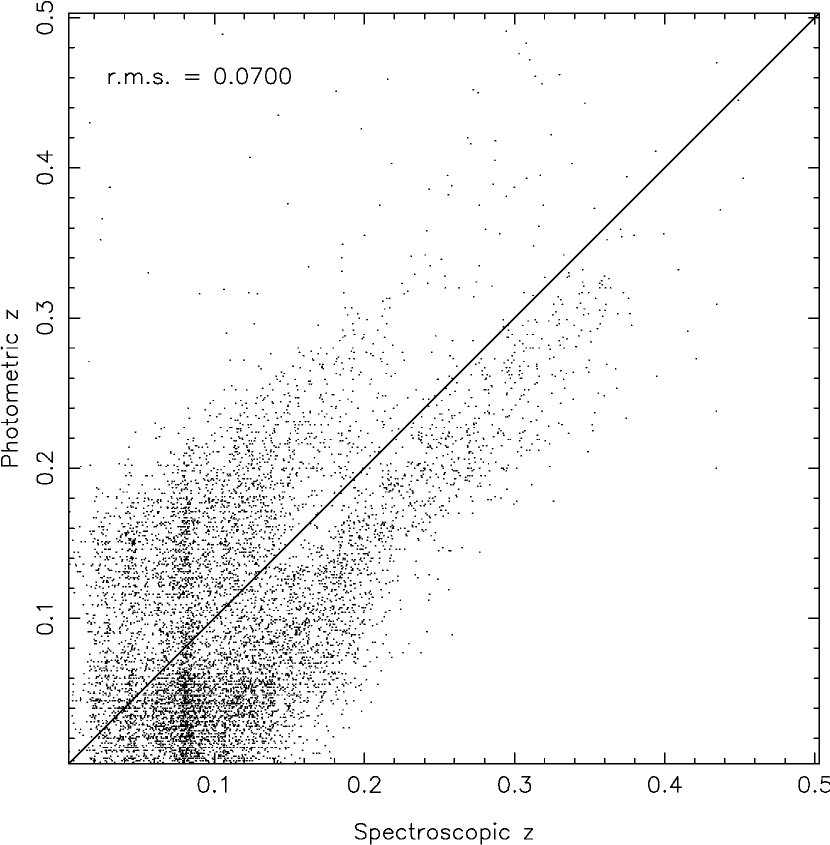
Hyperz (Bolzonella, Miralles, & Pelló, 2000) is a widely used template-based photometric redshift package. In order to more directly compare annz with the template-matching method, hyperz was applied to the same evaluation set using the CWW template SEDs (Coleman et al., 1980). It is clear from the results in Fig. 4 that not only is the rms dispersion in the photometric redshift considerably greater than that for annz, but there are also systematic deviations in the hyperz results. The SDSS consortium obtained similar accuracies to hyperz in their implementation of the basic template-fitting technique (the results labelled CWW and Bruzual-Charlot in Table 1 are for the respective template sets). With more sophisticated template-based methods they were able to improve on these errors: the result labelled Interpolated was obtained by first tuning the templates using the spectroscopic sample as a training set, then producing a continuous range of templates by interpolating between the tweaked SEDs. However, even “hybrid” methods such as this still do not match the accuracy achieved by the purely empirical methods (in the table these are: Polynomial, which uses a second-order polynomial as the fitting function, and Kd-tree, in which the training set is partitioned in colour-space and a separate second-order polynomial is fitted in each cell).

Figure 4.— Photometric redshift estimation using hyperz with the CWW template SEDs. This uses the same 10,000 galaxy sample as figure 2. There are obvious systematic deviations, with bands apparent above and below the $z_{\mathrm{phot}}=z_{\mathrm{spec}}$ line.

3.2. Extensions to the basic method

In this section more advanced use of annz is demonstrated. These examples use the LRG and main galaxy data from the SDSS Data Release 1 (DR1; Abazajian et al. 2003), split into training, validation and evaluation sets of respective sizes 50,000, 10,000 and 64,175. For these data the photometric redshift accuracy on the evaluation set when using the same basic method as in §3.1 was $\sigma_{\mathrm{rms}}=0.0238$.

3.2.1 Using additional inputs

One of the great advantages of empirical photometric redshift methods is the ease with which we can introduce additional observables into our parametrization of the photometric redshift. This is particularly true for annz; we simply add an extra input to our network architecture for each new parameter we wish to consider. annz treats these new inputs in exactly the same way as it does the galaxy magnitudes.

If the additional inputs contain useful information then the ANN will use this to improve the accuracy of its predictions. However, increasing the number of inputs to the ANN generally leads to a reduction in the generalization capabilities of the network (that is, its ability to make predictions for data on which it has not been trained). Thus, the inputs should be chosen carefully as non-informative inputs may actually lead to a worsened ANN performance: due to the increased dimensionality of the input space, larger training sets may be required and there will be an increased likelihood of converging to a local rather than the global minimum.

By way of example, the $r$-band 50 and 90 per cent Petrosian flux radii were added as two extra inputs to our ANN. These are the angular radii (concentric with the galaxy brightness distribution) containing the stated fraction of the Petrosian flux, and therefore contain information on the angular size of the galaxy (clearly a strongly distance-dependent property) and the concentration index (essentially the steepness of the galaxy brightness profile, which may help break degeneracies in the redshift-colour relationship). Running this extended data set through annz (using a committee of five 7:11:11:1 networks) produced a redshift estimation accuracy of $\sigma_{\mathrm{rms}}=0.0230$, an improvement of $\sim$3 per cent compared to the results based only on the magnitudes. In this example the improvement is small (mainly because the training sample already provided excellent redshift information), but it demonstrates well how straightforwardly the extra information could be included for consideration by annz.

3.2.2 Predicting spectral type

It is equally straightforward to train annz to make predictions for properties other than the redshift. Template-matching photometric redshift techniques have the useful side effect of assigning an estimated spectral type to each galaxy, in addition to estimating the redshift. Firth et al. (2003) demonstrated the use of ANNs to determine spectral types from broad-band photometry.

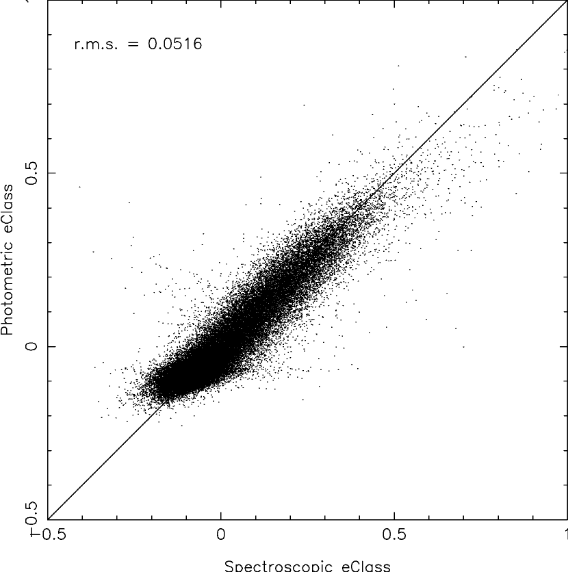
The spectroscopic catalogue of the SDSS includes a continuous parameter (eClass) indicating spectral type which ranges from approximately $-0.5$ (early types) to $1$ (late types). A 5:10:10:2 network architecture was used to attempt the simultaneous estimation of redshift and eClass from the photometry. The accuracy of the redshift estimation was very slightly poorer, $\sigma_{\mathrm{rms}}=0.0241$. The eClass was determined with an rms error of $\sigma_{\mathrm{rms}}=0.0516$ (Fig. 5).

Figure 5.— Results from using annz to predict the spectral type (in the form of the eClass parameter) simultaneously with the redshift for 64,175 galaxies from the SDSS Data Release 1.

3.3. More realistic conditions

Our example applications to the SDSS above are somewhat idealistic, since we are training and testing on samples with identical redshift, magnitude and galaxy species distributions. Furthermore, our training samples have thus far been very large. In this section less optimal training sets are used to investigate their impact on the photometric redshift accuracy.

3.3.1 Smaller training sets

The size of training sample needed will be strongly dependent on the range of redshifts and galaxy types in the target sample. The same evaluation set of 64,175 galaxies was submitted to networks trained on randomly selected samples of (i) 2000 galaxies and (ii) 200 galaxies. In both cases these samples were split equally into the training and validation sets. Committees of five 5:10:10:1 networks were used.

The photometric redshift accuracies were respectively (i) $\sigma_{\mathrm{rms}}=0.0263$ and (ii) $\sigma_{\mathrm{rms}}=0.0343$. In the first case the loss of accuracy is small, while the second case demonstrates well the problems associated with small training sets. The rarer classes of object in the target sample (e.g. here, those at high redshift) feature very sparsely (if at all) in the training set and so the network is unable to sensibly deal with these objects when they appear in the testing data. This leads to an increased number of outliers and, potentially, the introduction of systematic errors.

3.3.2 Biased training sets

For increasingly faint targets, acquiring good spectroscopy becomes increasingly difficult and eventually prohibitively expensive; this problem is the primary motivation for photometric redshifts. In practice then, the available spectroscopic training sample is likely to be somewhat brighter on average than the photometric target sets. However, the major stumbling block for empirical photometric redshift estimation techniques is the difficulty in applying them outside of the regions of parameter space which are well sampled by the training data: while the estimator ought to be able to interpolate within the training regime, extrapolating beyond is much more problematic. Ideally we would like to be able to train our estimator on bright galaxies, and then confidently apply it to faint galaxies.

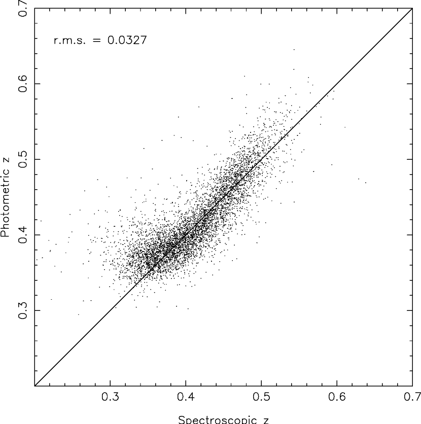
We can improve the ANN’s prospects by careful pre-selection of the data set. The Luminous Red Galaxies are a very uniform sample with respect to spectral types, since these early-type galaxies show little spectral evolution with redshift; this might be expected to make extrapolation a more manageable task. To assess the effectiveness of annz in this situation the LRG sample was split roughly in half by imposing a magnitude cut at $r=18.5$. The brighter subsample was further divided at random into training and validation sets of size 5000 and 2000 galaxies respectively. A committee of five 5:10:10:1 networks was trained on this data and then applied to the remaining $\sim 6000$ LRGs (for which the limiting magnitude is $r\approx 19.6$).

The results are shown in Fig. 6. The overall dispersion is $\sigma_{\mathrm{rms}}=0.0327$ which represents only a slight loss of accuracy when compared with results using a LRG training set selected over all magnitudes ($\sigma_{\mathrm{rms}}=0.0294$). Thus, in this particular case, annz is able to extrapolate with some success to around a magnitude fainter than is sampled by the training data.

Figure 6.— Results from training networks on LRGs with $r<18.5$, but applied to LRGs with strictly $r>18.5$ (note the change of intercept of the axes). The limiting magnitude for the LRGs is $r\approx 19.6$.

4. Conclusions

In appropriate circumstances, annz is a highly competitive tool for photometric redshift estimation. However, it does rely on the existence of a sufficiently large training set which is representative of the particular populations being studied. The package’s utility therefore lies particularly with large photometric surveys such as the SDSS, GOODS (Dickinson et al., 2001) or the VIRMOS-VLT Deep Survey (Le Fevre et al., 2003), some of which include spectroscopic surveys for subsets of the photometric catalogues (for example, of the eventual 100 million photometric objects which the SDSS expect to catalogue, 1 million will also have spectroscopy, and hence accurate redshifts).

A major problem for empirical photometric redshift estimators is the difficulty in extrapolating to regions of the input parameter space which are not well sampled by the training data. Care should be taken to match the training data to the target sample as closely as possible in terms of the magnitude and colour distributions of each. Use of an evaluation set is essential when applying annz to a new data set: the good performance demonstrated here on the SDSS data cannot be guaranteed on different data sets.

A potential solution to the problem of obtaining training sets when spectroscopy is difficult to obtain is to use simulated catalogues as training data (e.g. Vanzella et al. 2003). Since this requires the use of theoretical SEDs it introduces the disadvantages of the template-based methods, such as the need for precise calibration. However, the ANN approach has advantages over standard template-matching: simulated catalogues can contain galaxies representing a large range of complex star formation histories, dust extinction models and metallicities etc., giving fully Bayesian statistics, and ANNs allow much more flexible weighting to be applied to the filters than is possible with the simple $\chi^{2}$-weighting of standard template-matching.

References

- Abazajian et al. (2003) Abazajian, K., et al. 2003, AJ, 126, 2081
- Andreon et al. (2000) Andreon, S., Gargiulo, G., Longo, G., Tagliaferri, R., & Capuano, N. 2000, MNRAS, 319, 700
- Ball et al. (2003) Ball, N. M., Loveday, J., Fukugita, M., Nakamura, O., Okamura, S., Brinkmann, J., & Brunner, R. J. 2003, astro-ph/0306390
- Bertin & Arnouts (1996) Bertin, E., & Arnouts, S. 1996, A&AS, 117, 393
- Bishop (1995) Bishop, C. M. 1995, Neural Networks for Pattern Recognition (place of publication: Oxford University Press)
- Blum & Li (1991) Blum, E. K., & Li, L. K. 1991, Neural Networks, 4, 511
- Bolzonella et al. (2000) Bolzonella, M., Miralles, J.-M., & Pelló, R. 2000, A&A, 363, 476
- Bruzual & Charlot (1993) Bruzual, A. G., & Charlot, S. 1993, ApJ, 405, 538
- Coleman et al. (1980) Coleman, G. D., Wu, C.-C., & Weedman, D. W. 1980, ApJS, 43, 393
- Connolly et al. (1995) Connolly, A. J., Csabai, I., Szalay, A. S., Koo, D. C., Kron, R. G., & Munn, J. A. 1995, AJ, 110, 2655
- Csabai et al. (2003) Csabai, I., et al. 2003, AJ, 125, 580
- Dickinson et al. (2001) Dickinson, M., & GOODS Legacy Team. 2001, Bulletin of the American Astronomical Society, 33, 820
- Eisenstein et al. (2001) Eisenstein, D. J., et al. 2001, AJ, 122, 2267
- Fernández-Soto et al. (1999) Fernández-Soto, A., Lanzetta, K. M., & Yahil, A. 1999, ApJ, 513, 34
- Firth et al. (2003) Firth, A. E., Lahav, O., & Somerville, R. S. 2003, MNRAS, 339, 1195
- Jones (1990) Jones, L. K. 1990, Proceedings of the IEEE, 78, 1586
- Lahav et al. (1996) Lahav, O., Naim, A., Sodré, L., & Storrie-Lombardi, M. C. 1996, MNRAS, 283, 207
- Le Fevre et al. (2003) Le Fevre, O., Vettolani, G., Maccagni, D., Mancini, D., Mazure, A., Mellier, Y., & Picat, J. P. 2003, Proc. SPIE, 4834, 173
- Sowards-Emmerd et al. (2000) Sowards-Emmerd, D., Smith, J. A., McKay, T. A., Sheldon, E., Tucker, D. L., & Castander, F. J. 2000, AJ, 119, 2598
- Stoughton et al. (2002) Stoughton, C., Lupton, R. H., Bernardi, M., Blanton, M. R., Burles, S., & Castander, F. J. 2002, AJ, 123, 485
- Strauss et al. (2002) Strauss, M. A., Weinberg, D. H., Lupton, R. H., & Narayanan, V. K. 2002, AJ, 124, 1810
- Vanzella et al. (2003) Vanzella, E., et al. 2003, astro-ph/0312064
- York et al. (2000) York, D. G., Adelman, J., Anderson, J. E., & Anderson, S. F. 2000, AJ, 120, 1579