Detection of Weak Gravitational Lensing by Large-scale Structure

Abstract

We report a detection of the coherent distortion of faint galaxies arising from gravitational lensing by foreground structures. This “cosmic shear” is potentially the most direct measure of the mass power spectrum, as it is unaffected by poorly-justified assumptions made concerning the biasing of the distribution. Our detection is based on an initial imaging study of 14 separated $8^{\prime}\times 16^{\prime}$ fields observed in good, homogeneous conditions with the prime focus EEV CCD camera of the 4.2m William Herschel Telescope. We detect an rms shear of 1.6% in $8^{\prime}\times 8^{\prime}$ cells, with a significance of $3.4\sigma$. We carefully justify this detection by quantifying various systematic effects and carrying out extensive simulations of the recovery of the shear signal from artificial images defined according to measured instrument characteristics. We also verify our detection by computing the cross-correlation between the shear in adjacent cells. Including (gaussian) cosmic variance, we measure the shear variance to be $(0.016)^{2}\pm(0.012)^{2}\pm(0.006)^{2}$, where these $1\sigma$ errors correspond to statistical and systematic uncertainties, respectively. Our measurements are consistent with the predictions of cluster-normalised CDM models (within $1\sigma$) but a COBE-normalised SCDM model is ruled out at the $3.0\sigma$ level. For the currently-favoured $\Lambda$CDM model (with $\Omega_{m}=0.3$), our measurement provides a normalisation of the mass power spectrum of $\sigma_{8}=1.5\pm 0.5$, fully consistent with that derived from cluster abundances. Our result demonstrates that ground-based telescopes can, with adequate care, be used to constrain the mass power spectrum on various scales. The present results are limited mainly by cosmic variance, which can be overcome in the near future with more observations.

1 Introduction

Determining the large scale distribution of matter remains a major goal of modern cosmology. Comparisons between theory and observations are hampered fundamentally by the fact that the former is concerned with dark matter whereas the latter usually probes luminous matter, particularly when the distribution is probed by galaxies and clusters. By contrast, gravitational lensing provides direct information concerning the total mass distribution, independently of its state and nature. As a result, lensing has had considerable impact in studies of cluster mass distributions (see reviews by Fort & Mellier 1994, Schneider 1996) and observational limits have improved significantly. Weak shear has now been detected $>$1.5 Mpc from the centre of the cluster Cl0024+16 (Bonnet et al. 1994), and in a supercluster (Kaiser et al. 1998).

Weak lensing by large-scale structure also produces small coherent distortions in the images of distant field galaxies (see Mellier 1999; Kaiser 1999; Bartelmann & Schneider 1999 for recent reviews). A measurement of this effect on various scales (defined as ‘cosmic shear’) would provide invaluable cosmological information (Kaiser 1992; Jain & Seljak 1997; Kamionkowski et al. 1997; Kaiser 1998; Hu & Tegmark 1998; Van Waerbeke et al. 1998). In particular, it would yield a direct measure of the power spectrum of density fluctuations along the line of sight and thus provide an independent constraint on large scale structure models and cosmological parameters.

Because of its small amplitude (a few percent on arcmin scales for favoured CDM models), cosmic shear has however been difficult to detect. In a pioneering paper, Mould et al. (1994) attempted to detect the coherent distortion of $R\sim$26 field galaxies over a 9.6 arcmin diameter field and found an upper limit quoted in terms of the rms shear at the 4% level. A search for this effect is the object of active observational effort (Van Waerbeke et al. 1998; Refregier et al. 1998; Seitz et al. 1998; Rhodes et al. 1999; Kaiser 1999). At present however, no unambiguous detections of cosmic shear have been reported (see however the limited results of Villumsen 1995; Schneider et al. 1998).

A fundamental limitation of narrow field imaging as a probe of cosmic shear is that arising from cosmic variance, i.e. the fluctuation in the lensing signal measured with a limited number of pencil beam sight lines. Only through the analysis of image fields in many statistically-independent directions can this variance be overcome. Prior to such a measurement, it is important to demonstrate a reliable detection strategy, particularly in the presence of significant instrumental and other systematic effects.

In this paper, we report the detection of a cosmic shear signal with 14 separated $16^{\prime}\times 8^{\prime}$ fields observed with the 4.2m William Herschel Telescope (WHT). We provide a detailed treatment of systematic effects and of the shear measurement method. We test our results with numerical simulations of lensed images and quantify both our statistical and systematic errors. We discuss the consequence of our measurement for the normalisation of the mass power spectrum. Subsequent papers will extend this technique to a larger number of fields, reducing the limitations caused by cosmic variance.

This paper is organised as follows. In §2, we introduce the theory of weak lensing in the context of a cosmic shear survey. In §3 we discuss our observational strategy for detecting it and describe our observations taken at the WHT and the routine aspects of data reduction. In §4, we describe the generation of the object catalogue and how the image parameters were measured. In §5 we discuss and characterise distortions introduced by the telescope optics. In §6 we discuss the point spread function and present our shear measurement method, alongside an important comparison with the same analysis conducted with simulated data (§7). In §8, we describe the estimator used for measuring the shear variance and the cross-correlation between adjacent cells. In §9, we present our results. Our conclusions are summarised in §10.

2 Theory

2.1 Distortion Matrix

Gravitational lensing by large scale structure produces distortions in the image of background galaxies (see Mellier 1999; Kaiser 1999; Bartelmann & Schneider 1999 for recent reviews). These distortions are weak (about 1%) and can be fully characterised by the distortion matrix

$$\Psi_{ij}\equiv\frac{\partial(\delta\theta_{i})}{\partial\theta_{j}}\equiv\left(\begin{array}[]{cc}\kappa+\gamma_{1}&\gamma_{2}\\ \gamma_{2}&\kappa-\gamma_{1}\\ \end{array}\right),$$ (1)

where $\delta\theta_{i}({\mathbf{\theta}})$ is the displacement vector produced by lensing on the sky. The convergence $\kappa$ describes overall dilations and contractions. The shear $\gamma_{1}$ ($\gamma_{2}$) describes stretches and compressions along (at $45^{\circ}$ from) the x-axis.

The distortion matrix is directly related to the matter density fluctuations along the line of sight by

$$\Psi_{ij}=\int_{0}^{\chi_{h}}d\chi~{}g(\chi)\partial_{i}\partial_{j}\Phi$$ (2)

where $\Phi$ is the Newtonian potential, $\chi$ is the comoving distance, $\chi_{h}$ is the comoving distance to the horizon, and $\partial_{i}$ is the comoving derivative perpendicular to the line of sight. The radial weight function $g(\chi)$ is given by

$$g(\chi)=2\int_{\chi}^{\chi_{h}}d\chi^{\prime}~{}n(\chi^{\prime})\frac{r(\chi)r(\chi^{\prime}-\chi)}{r(\chi^{\prime})},$$ (3)

where $r$ is the comoving angular diameter distance, and $n(\chi)$ is the probability of finding a galaxy at comoving distance $\chi$ and is normalised as $\int d\chi n(\chi)=1$. If the galaxies all lie at a single distance $\chi_{s}$, $n(\chi)=\delta(\chi-\chi_{s})$ and

$$g(\chi)=2\frac{r(\chi)r(\chi_{s}-\chi)}{r(\chi_{s})}$$ (4)

In practice, this approximation is accurate to within 10%, if $\chi_{s}$ is set to the median distance of the galaxy sample. This is adequate given the median redshift of our galaxy sample is itself uncertain by about 25% (see §3.2), yielding an uncertainty in the predicted rms shear of about 20% (see Eq. [20] below).

2.2 Power Spectrum

The amplitude of the cosmic shear can be quantified statistically by computing its 2-dimensional power spectrum (Jain & Seljak 1997; Kamionkowski et al. 1997; Schneider et al. 1997; Kaiser 1998). For this purpose, we consider the Fourier transform of the shear field

$$\widetilde{\gamma_{i}}({\mathbf{l}})=\int d^{2}\theta~{}\gamma_{i}({\mathbf{\theta}})e^{i{\mathbf{l}\cdot\theta}}$$ (5)

The shear power spectrum $C_{{\mathbf{l}}}^{ij}$ is defined by

$$\langle\widetilde{\gamma_{i}}({\mathbf{l}})\widetilde{\gamma_{j}}({\mathbf{l}^{\prime}})\rangle=(2\pi)^{2}\delta^{(2)}({\mathbf{l}}-{\mathbf{l}^{\prime}})C_{{\mathbf{l}}}^{ij}$$ (6)

where $\delta^{(2)}$ is the 2-dimensional Dirac-delta function, and the brackets denote an ensemble average. It is also useful to define the scalar power spectrum $C_{l}=C_{{\mathbf{l}}}^{11}+C_{{\mathbf{l}}}^{22}$ for the shear amplitude by

$$\langle\widetilde{\gamma_{i}}({\mathbf{l}})\widetilde{\gamma_{i}}({\mathbf{l}^{\prime}})\rangle=(2\pi)^{2}\delta^{(2)}({\mathbf{l}}-{\mathbf{l}^{\prime}})C_{{\mathbf{l}}},$$ (7)

where the summation convention was used.

Applying Limber’s equation in Fourier space (Kaiser 1998) to Equation (2) and using the Poisson equation, we can express the shear power spectrum $C_{l}$ in terms of the 3-dimensional power spectrum $P(k,\chi)$ of the mass fluctuations $\delta\rho/\rho$ and obtain

$$C_{l}=\frac{9}{16}\left(\frac{H_{0}}{c}\right)^{4}\Omega_{m}^{2}\int_{0}^{\chi_{h}}d\chi~{}\left[\frac{g(\chi)}{ar(\chi)}\right]^{2}P\left(\frac{l}{r},\chi\right),$$ (8)

where $a$ is the expansion parameter, and $H_{0}$ and $\Omega_{m}$ are the present value of the Hubble constant and matter density parameter, respectively. After noting that $C_{l}$ is also equal to the power spectrum of the convergence $\kappa$, we find that this expression agrees with that of Schneider et al. (1997). The component-wise power spectrum is given by

$$C_{{\mathbf{l}}}^{ij}=u_{i}(\lambda)u_{j}(\lambda)C_{l}$$ (9)

where $u_{i}(\lambda)=\{\cos(2\lambda),\sin(2\lambda)\}$ and $\lambda$ is the angle of the vector ${\mathbf{l}}$, counter-clockwise from the $l_{1}$-axis.

A measurement of the power spectrum enables differentiation between the different cosmological models listed in Table 1. Standard Cold Dark Matter (SCDM) is approximately COBE-normalised (Bunn & White 1997), while the other variants are approximately cluster normalised ($\sigma_{8}\Omega_{m}^{.53}=0.6\pm 0.1$; Viana & Liddle 1996). For each model we compute the non-linear power spectrum using the fitting formula of Peacock & Dodds (1996). The resulting power spectra are shown in Figure 1 for sources observed at $z_{s}=1$.

Table 1: Cell-averaged statistics for each cosmological model (with $z_{s}=1$)

Model	$\Omega_{m}$	$\Omega_{\Lambda}$	$\sigma_{8}$	$\Gamma$	$\sigma_{\gamma}$ (%)	$\sigma_{\times}$ (%)	$\sigma_{\times 1}$ (%)	$\sigma_{\times 2}$ (%)
SCDM	1.0	0	1	0.50	2.60	1.62	1.23	1.05
$\tau$CDM	1.0	0	0.6	0.25	1.25	0.86	0.64	0.58
$\Lambda$CDM	0.3	0.7	1	0.25	1.15	0.71	0.54	0.46
OCDM	0.3	0	1	0.25	1.04	0.62	0.48	0.39

Figure 1: Shear power spectrum for each cosmological model and for sources at $z_{s}=1$. Note that the SCDM spectrum is larger due to its higher normalisation.

2.3 Cell-Averaged Statistics

For our measurement, we will consider statistics of the shear averaged over angular cells on the sky. This has the advantage of diminishing the impact of systematic effects (Rhodes et al. 1999) and allows extension in later surveys to minimise cosmic variance. The average shear $\overline{\gamma}_{i}$ in a cell can be written as

$$\overline{\gamma}_{i}=\int d^{2}\theta~{}W({\mathbf{\theta}})\gamma_{i}({\mathbf{\theta}})$$ (10)

where $W({\mathbf{\theta}})$ is the cell window function and is normalised as $\int d^{2}\theta~{}W({\mathbf{\theta}})=1$.

It is convenient to define the Fourier transform of the window function as

$$\widetilde{W}_{{\mathbf{l}}}=\int d^{2}\theta~{}W({\mathbf{\theta}})e^{i{\mathbf{l}\cdot\theta}}.$$ (11)

For a square cell of side $\alpha$, this is

$$\widetilde{W}_{{\mathbf{l}}}=\left(\frac{\sin(\alpha l_{1})}{\alpha l_{1}}\right)\left(\frac{\sin(\alpha l_{2})}{\alpha l_{2}}\right),$$ (12)

To a good approximation, we can ignore the small azimuthal dependence of the window function and approximate

$$\widetilde{W}_{l}\simeq\left(\frac{\sin(\alpha l/\sqrt{2})}{\alpha l/\sqrt{2}}\right)^{2}.$$ (13)

Let us consider 2 cells separated by an angle ${\mathbf{\theta}}$. We are interested in the correlation function

$$w_{ij}({\mathbf{\theta}})\equiv\langle\overline{\gamma}_{i}(0)\overline{\gamma}_{j}({\mathbf{\theta}})\rangle$$ (14)

As is the case in our experiment, we take the separation vector ${\mathbf{\theta}}$ to lie along the $\theta_{1}$-axis (or equivalently along the $\theta_{2}$-axis). By taking Fourier transforms and using Equation (6), we thus obtain

$$w_{ij}({\mathbf{\theta}}) \simeq \frac{1}{4\pi}\int_{0}^{\infty}dl~{}lC_{l}\left|\widetilde{W}_{l}\right|^{2}\times$$ (17)

$$\left(\begin{array}[]{cc}J_{0}(l\theta)+J_{4}(l\theta)&0\\ 0&J_{0}(l\theta)-J_{4}(l\theta)\\ \end{array}\right).$$

As noted above, we have ignored the azimuthal dependence of the window function $\widetilde{W}_{l}$. In particular, the shear variance $\sigma_{\gamma}^{2}\equiv\langle\overline{\gamma}^{2}\rangle=w_{11}(0)+w_{22}(0)$ is given by

$$\sigma_{\gamma}^{2}=\frac{1}{2\pi}\int_{0}^{\infty}dl~{}lC_{l}\left|\widetilde{W}_{l}\right|^{2}.$$ (18)

We will denote the component-wise covariances between two adjacent cells by

$$\sigma_{\times 1}^{2}\equiv w_{11}(\alpha),~{}~{}~{}\sigma_{\times 1}^{2}\equiv w_{22}(\alpha),$$ (19)

and their modulus by $\sigma_{\times}^{2}\equiv\sigma_{\times 1}^{2}+\sigma_{\times 2}^{2}$. The values of these statistics for each model are listed in Table 1 for our cell size of $\alpha=8^{\prime}$. The rms shear is of the order of 1% for the cluster-normalised models and of about 2% for the COBE-normalised model. The cross-correlation rms is about half the zero-lag value (c.f. Schneider et al. 1997).

Figure 2 shows the dependence of $\sigma_{\gamma}$ on the source redshift $z_{s}$ and $\sigma_{8}$ for the $\Lambda$CDM model (again for $\alpha=8^{\prime}$). The range chosen approximately reflects the likely uncertainty in these parameters for our experiment. Importantly, the rms shear is more sensitive to $\sigma_{8}$. A 10% uncertainty in the source redshift results in a 8% uncertainty in $\sigma_{\gamma}$. For this model, the dependence of $\sigma_{\gamma}$ is very well approximated by

$$\sigma_{\gamma}\simeq 0.0115z_{s}^{0.81}\sigma_{8}^{1.25},$$ (20)

in agreement with the scaling laws of Jain & Seljak (1997).

Figure 2: Dependence of the rms shear on the source redshift $z_{s}$ and the power spectrum normalisation $\sigma_{8}$. The cell was chosen to be a square of side $\alpha=8^{\prime}$.

3 Data

3.1 Survey Strategy

In order to detect and ultimately measure the cosmic shear, an array of deep imaging fields is required. These must be randomly placed on the sky to provide a fair sample, and should be well separated in order to be statistically independent, from the point of view of cosmic variance. As mentioned in §1, it is expedient to distinguish between a detection based on a careful analysis of a few fields, noting carefully the systematic effects, before embarking upon an exhaustive measurement survey utilising a larger number of fields to beat down the uncertainties arising from cosmic variance. With these factors in mind, we now discuss our strategy and observations using the William Herschel Telescope (WHT).

A bank of appropriate fields were selected for observation with the WHT prime focus CCD Camera (field of view 8’ $\times$ 16’, pixel size 0.237”, EEV CCD) in the $R$ band. This photometric band offers the deepest imaging for a given exposure time with minimal fringing. Fields were selected using the Digital Sky Survey by choosing coordinates randomly within the range appropriate for the time of observations. Each field was retrospectively checked to see whether it contained large galaxies ($\gg 5$ arcsec) (which would occult a significant fraction of the imaging field) or prominent groups/clusters (located using the NASA/IPAC Extragalactic Database) on a scale comparable to that under study ($\simeq$8 arcmin). There is, of course, a danger of over-compensating by exclusion in this respect but, fortunately, none of the originally-chosen fields were discarded according to the above criteria.

The fields were further required to be $>5^{\circ}$ away from one other, in order to ensure statistical independence (c.f. figure 1, where the power is small for $l<10$).

Using the APM and GCC catalogues, we ensured that the fields contained no stars with $R<11$ (in order to avoid large areas of saturation and ghost images). On the other hand, we required the fields to contain $\simeq 200$ stars with $R<22$ in order to map carefully the anisotropic PSF and the camera distortion across the field of view. In order to achieve this, the fields were chosen to be at intermediate Galactic latitudes ($30^{\circ}<b<70^{\circ}$; see Table 2). A calibration of the stellar density at limits fainter than the APM and GCC catalogues was obtained from a test WHT image (see below).

The final constraint on field position was our desire to observe each field within $20^{\circ}$ of the telescope’s zenith during the observing run; this reduces image distortion introduced by telescope and instrument flexure. This criterion was relaxed for the fields VLT1, CIRSI1 and CIRSI2 (see nomenclature below).

Table 2 summarises the positions and Galactic latitude of the fields which are used in this paper. Two fields are in common with the VLT (Mellier et al., in preparation) and HST STIS (Seitz et al. 1998) cosmic shear programmes, allowing future comparisons with these programmes. A further two fields spanned the Groth Strip (Groth et al. 1998; Rhodes 1999) a deep survey conducted with HST, which has previously been studied for cosmic shear detection (Rhodes et al. 1999). Finally, two fields were chosen to be in common with the current CIRSI photometric redshift survey (Firth et al., in preparation) to give us clearer understanding of the redshift distribution of objects in our fields at a later date.

Table 2: Field Coordinates (equinox 2000) and Properties

Field name	RA (h:m:s)	Dec (d:m:s)	Galactic	Seeing	Magnitude	Median	No. Survey Galaxies
			latitude	(arcsec)	limit	magnitude	$(8^{\prime}\times 16^{\prime}field$)
			(deg)		(imcat $5\sigma)$	of survey
						galaxies
WHT0	02:03:09.31	11:30:20.0	-47.6	0.59	26.2	23.1	1550
WHT3	14:00:15.00	10:13:40.0	66.6	0.82	26.2	23.3	2141
WHT5	14:50:46.67	20:18:03.2	61.9	0.76	26.5	23.7	2181
WHT7	15:13:40.86	36:31:30.8	58.6	0.83	25.9	23.0	1354
WHT11	16:31:44.28	27:56:30.0	41.6	0.85	26.0	23.3	1379
WHT12	16:37:20.00	20:46:30.0	38.4	0.90	26.0	23.3	1855
WHT14	16:51:15.38	25:46:44.0	36.8	0.99	25.9	23.2	1701
WHT16	17:13:40.00	38:39:19.0	34.9	0.78	25.8	23.4	2074
WHT17	14:24:38.10	22:54:01.0	68.5	0.63	27.3	24.5	2287
VLT1	12:28:18.50	02:10:05.0	64.4	0.71	26.4	23.6	1721
VLT2	15:28:43.00	10:14:20.0	49.3	0.79	26.1	23.4	2093
CIRSI1	12:05:35.01	-07:43:00.0	60.1	1.14	25.4	22.6	1192
CIRSI2	15:23:37.00	00:15:00.0	60.4	0.76	26.3	23.5	1824
GROTH1	14:17:18.74	52:20:18.5	53.4	0.78	26.1	23.4	2237
GROTH2	14:15:35.00	52:08:48.0	44.7	0.89	26.1	23.6	1195

An exposure time of 1 hour on the WHT enables the detection of $R$=26 objects with a signal-to-noise of 5.8 in 0.8” seeing. This limit should correspond to a median redshift of about $z_{s}\simeq$1.2. In our eventual analysis, we will introduce a brighter limit so as to keep only resolved galaxies (referred to as the survey sample). This serves to reduce the median redshift to about 0.8 (see $\S$9.3). We however note from figure 2 that our expected shear signal is not very sensitive to median redshift ($\sigma_{\gamma}\propto z_{s}^{0.8}$). In §9, we will show that the resulting depth is still sufficient to detect the lensing signal.

3.2 Observations

We observed 14 selected fields with the WHT during the nights of 13-16 May 1999. For each field, a total of 4 exposures in $R$, each of 900s, was taken. All fields were observed as they passed through the meridian.

Each exposure on a given field was offset by 10” from its predecessor in order to remove cosmetic defects and cosmic rays, and to measure the optical distortion of the telescope and camera (see §5 and §6). All but two of the fields were observed with the long axis of the CCD pointing East-West; the exception being the two Groth fields, for which a $45^{\circ}$ rotation (i.e. North-West orientation) was effected to align the WHT exposures with the HST survey (Groth et al. 1998; Rhodes 1999). Bias frames and sky flats were taken at the beginning and end of each night, and standard star observations were interspersed with the science exposures. The median seeing on our used exposures is 0.81”; one exposure with seeing $>1.2$” was excluded.

Table 2 lists the seeing and ’imcat’ magnitudes corresponding to $5\sigma$ detections for each field. An ’imcat’ signal-to-noise (see Section 7) of 5.0 corresponds to a median $R$=26.1; the median magnitude of galaxies on a field is $R$=25.2. To measure the shear, a number of cuts have to be applied to our object catalog (see §6). Table 2 also lists the median magnitude of our final sample. At our final subsample limit of $R$=23.4, the median redshift is $\simeq 0.8\pm 0.2$ (Cohen et al 2000, $\S$9.3). The median number density of adopted survey sources is 14.3 arcmin^-2 (see section 6).

In addition to the 13 useful fields, we had already obtained a test field (WHT0) in service time, and were also kindly given access to a suitable archival field, WHT17. Both were taken in good conditions: WHT0 is a 1 hour exposure in the $I$ band, whereas WHT17 is a 1.5 hour exposure in $R$ (chosen to include a known quasar). Removing these fields does not significantly alter our results. In terms of uniformity, apart from the deeper WHT17 field, the standard deviation in limiting magnitude is $\simeq$0.2 mag which we consider acceptable for our survey. The error on magnitude zero point derived from standard stars is at the much lower level of 0.03 mag.

3.3 Data Reduction

The reduction of these deep images proceeded along a standard route. A median-combined bias frame was subtracted from the skyflats and science exposures, and all such exposures were divided by a median unit-normalised sky-flat. Although the survey exposures were undertaken in the $R$ band to avoid fringing, fringing is still detected at a 0.5% sky level. In order to remove these fringes, which could potentially introduce structure into the image ellipticities, all long dithered exposures for a given night ($>15$ exposures per night) were stacked without offsetting with a sigma-clipping algorithm. This results in a fringe frame mapping the background fringes but devoid of foreground objects. The fringe frame for the relevant night was then subtracted from each science exposure individually, subtracting off the multiple of the fringe frame found to minimise the rms background noise. After applying this technique, the fringes are entirely imperceptible, any residue having an amplitude within the sky background noise. We experimented with automated and hand- subtraction of the fringes and verified that this had no noticeable effect on our shear analysis.

The mean linear astrometric offset (in fractional number of pixels) between the four exposures was found by producing SExtractor (Bertin & Arnoults 1996) catalogues for each exposure, containing typically 2000-3000 objects. We used the mean offsets of the matched objects to align the fields. The images were shifted by the corresponding non-integer number of pixels using IRAF’s imshift routine, taking linear combinations of neighbouring pixels to effect the non-integer pixel shifts. As discussed in §5, we find no need to rotate the exposures with respect to each other, or to make further astrometric distortions to compensate for the optical distortion of the instrument.

The resulting four exposures for each science field were stacked with sigma-clipping. Since each exposure is 10” away from the others, bad columns and cosmic rays were rejected. The images were examined visually and remaining defective pixels (e.g. a star just outside field of view leading to light leakage onto an area of the CCD; or highly saturated stars) were flagged as potentially unreliable.

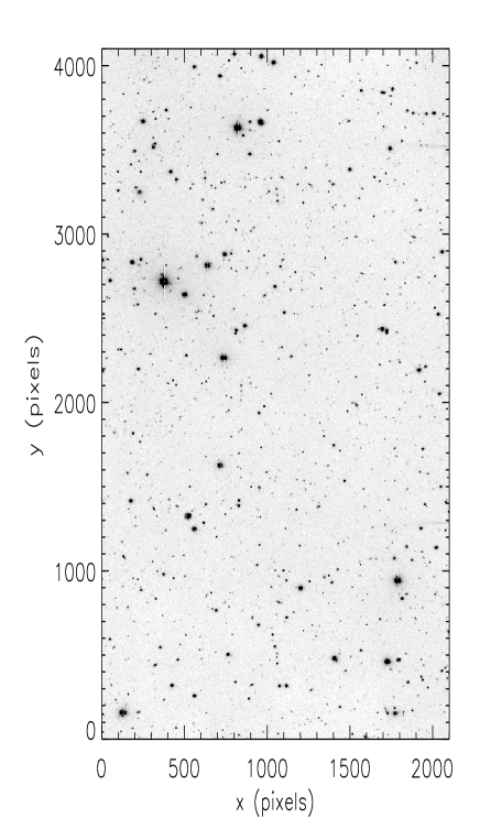
Figure 3: Example reduced image (CIRSI2); the field of view is 8’$\times$ 16’. Note that in our analysis, we divide each such field into two 8’ $\times$ 8’ cells.

4 Image Analysis

We are now ready to measure the ellipticities of the galaxies on each field, and to apply the necessary corrections in order to take into account the smearing effect of the atmosphere (‘seeing’) plus tracking and other instrumental distortions introduced by the telescope and camera optics. Only then can we ascertain the true cosmic shear by averaging the ellipticity distributions of the corrected galaxies. If no shear were present on a given field, the mean ellipticity would be zero, within the noise expected from the non-circularity of galaxies and pixelisation effects. If a shear is present, the mean ellipticity will be significant, especially when results are combined from many fields.

A number of methods have recently been proposed to derive the shear from galaxy shapes (Kaiser et al 1995; Rhodes et al. 1999; Kuijken 1999; Kaiser 1999). Here we choose the most documented method, namely the KSB formalism proposed by Kaiser et al (1995) and further developed in Luppino & Kaiser (1997) and Hoekstra et al. (1998). While this method is known to have a number of shortcomings (Rhodes et al. 1999; Kuijken 1999; Kaiser 1999), it is nevertheless the simplest and is readily available. As we will show in §7 using simulations, the method is suitable for our purposes, after a number of precautions are taken (see Bacon et al. 2000 for more details). We therefore use this method as provided by the imcat software, a numerical implementation of Kaiser et al. 1995.

The first task in this process is to detect all objects present on the fields down to the background noise level, and to measure their shapes. We then wish to measure their polarisabilities i.e. measures of how each is affected by an isotropic smear (due principally to the atmosphere), an anisotropic smear (due to tracking errors at the telescope and local coaddition errors due to astrometric distortion) and shear (both the real gravitational shear and optical distortions due to the telescope and camera optics). One should note the distinction between smear and shear: a smear is a convolution of the image with a kernel, whereas a shear is a stretching of the image which conserves surface brightness. We will now describe the method for finding objects, and for measuring their ellipticities and their shear and smear polarisabilities.

4.1 Object Detection

For the purpose of detecting cosmic shear, it is expedient to divide each of our fields into 2 $8^{\prime}\times 8^{\prime}$ cells, since the signal is stronger on smaller scales (see Figure 1). Furthermore, the mean shear correlation between two adjacent cells is expected to be about $0.7$% (see Section 2), and can thus be used to independently verify our results.

We use the imcat software to find objects in each cell, and to measure their ellipticities, radii, magnitudes, and polarisabilities. The hfindpeaks routine convolves the cell with Mexican hat functions of varying size, and maximally significant peaks in surface brightness after convolution are designated objects. The radius of the hat giving the largest signal to noise $\nu$ for a given galaxy is attributed to that galaxy as its filter radius $r_{g}$. The local sky background is estimated by the getsky routine, and aperture photometry is carried out on the objects, determining magnitude and half-light radius $r_{h}$ for all objects using the apphot routine.

4.2 Shape Measurement

Using the getshapes routine, we then measure the weighted quadrupole moments of each object which are defined as

$$I_{ij}\equiv\int d^{2}x~{}w(x)x_{i}x_{j}I(\mbox{\boldmath$x$})$$ (21)

where $I$ is the surface brightness of the object, $x$ is angular distance from object centre, and $w(x)$ is a Gaussian weight function of scale length equal to $r_{g}$. In this fashion we obtain ellipticity components

$$e_{i}\equiv I_{i}/T,$$ (22)

where

$$I_{1}\equiv I_{11}-I_{22},\;\;I_{2}\equiv 2I_{21},\;\;T\equiv I_{11}+I_{22}.$$ (23)

We can further define $e\equiv(e_{1}^{2}+e_{2}^{2})^{\frac{1}{2}}$, where $e_{1}=e\cos{2\phi}$ and $e_{2}=e\sin{2\phi}$, where $\phi$ is the position angle associated with the elongation direction of the object (anticlockwise from x-axis). The trace $T$ of the quadrupole moments provides a measure for the rms radius $d$ of the object, which we define as

$$d^{2}\equiv\frac{1}{2}(I_{11}+I_{22})/I_{0},$$ (24)

where $I_{0}\equiv\int d^{2}x~{}w(x)I(\mbox{\boldmath$x$})$ is the flux of the object.

4.3 Polarisability

The imcat software also enables us to calculate the smear and shear polarisabilities. In the following, we briefly review their function. It is possible (see e.g. KSB 95 Appendix) to calculate the effects of anisotropic smearing, by replacing the image $I(\mbox{\boldmath$x$})$ in (21) with a convolved (i.e. anisotropically smeared) image $I^{\prime}(\mbox{\boldmath$x$})$ and by finding the effect on the original $e_{i}$. It is found that the galaxy ellipticity $e^{g}_{\rm smeared}$ can be corrected for the smear as

$$e^{g}_{\rm corrected}=e^{g}_{\rm smeared}-P^{g}_{sm}p,$$ (25)

where the ellipticities are understood to denote the relevant 2-component spinor $e_{i}$, and $p$ is a measure of PSF anisotropy. The tensor $P^{g}_{sm}$ is the smear polarisability, a $2\times 2$ matrix with components involving various moments of surface brightness. Since for stars $e^{*}_{\rm corrected}=0$, we can set $p=(P^{*}_{sm})^{-1}e^{*}_{\rm smeared}$, and find

$$e^{g}_{\rm corrected}=e^{g}_{\rm smeared}-P^{g}_{sm}(P^{*}_{sm})^{-1}e^{*}_{\rm smeared}$$ (26)

In this fashion, we can correct a galaxy ellipticity for the effect of anisotropic smearing, using the smear polarisability $P^{g}_{sm}$.

In a similar manner, we can calculate the effect of a shear, however it is induced. Replacing the image $I(\mbox{\boldmath$x$})$ in (21) with a weakly sheared image, we find that

$$e^{g}_{\rm sheared}=e^{g}_{\rm initial}+P^{g}_{sh}\gamma,$$ (27)

where $\gamma$ denotes the two component shear (Eq. [32]), and $P^{g}_{sh}$ is the shear polarisability, a $2\times 2$ matrix with components involving various moments of surface brightness (different from $P^{g}_{sm}$ above).

In practice, the lensing shear takes effect before the circular smearing of the PSF. Luppino and Kaiser (1997) showed that the pre-smear shear $\gamma$ averaged over a field can be recovered using

$$\langle{P_{\gamma}}\gamma\rangle=\langle{e^{g}_{\rm corrected}}\rangle$$ (28)

where

$$P_{\gamma}=P_{sh}^{g}-\frac{P_{sh}^{*}}{P_{sm}^{*}}P_{sm}^{g}.$$ (29)

Here, $e^{g}_{\rm corrected}$ is the galaxy ellipticity corrected for smear, as in equation (25), and $P_{sh}^{*}$ and $P_{sm}^{*}$ are the shear and smear polarisabilities calculated for a star interpolated to the position of the galaxy in question. The interpretation of the division in this equation is a matter of debate; our adopted procedure will be found in Section 7. With the smear and shear polarisabilities calculated by imcat, we can therefore find an estimator for the mean shear in a given cell.

In summary, we can derive a catalogue of objects on a cell. For every object, we determine its centroid, magnitude, half-light and filter radii, ellipticity components and polarisabilities as defined above. We can now use these catalogues to understand and correct for systematic effects, particularly for instrumental distortion and PSF-induced effects.

5 Instrumental Distortions

The instrumental distortion induced by the optical system of the telescope must be accounted for. If left uncorrected, this effect can indeed produce both a spurious shear and a smearing during the coadding process. In the following, we first present our method to measure the distortion using dithered astrometric frames. We then apply this method to our WHT fields and compare our measured distortion field to that predicted by the WHT Prime Focus manual (Carter & Bridges 1995). We then show how the coadding smear can be computed from the astrometric frames. We finally quantify the impact of these effects on our lensing measurement.

5.1 Measurement of the Astrometric Distortion

The distortion field introduced by the telescope and camera optics can be measured from the astrometric shifts of objects observed in several frames offset by known amounts. Let ${\mathbf{x}}$ be the true position of an object. Let ${\mathbf{x}}^{f}$ be its position observed in frame $f$, without any correction for the camera distortion. The observed position can be written as

$${\mathbf{x}}^{f}={\mathbf{x}}+{\mathbf{\delta}x}({\mathbf{x}}-{\mathbf{\overline{}}{x}}^{f})$$ (30)

where ${\mathbf{\delta}x}$ is the displacement produced by the distortion. The vector ${\mathbf{\overline{}}{x}}^{f}$ is the position of the centre of frame $f$, and can be measured as the average position of all the objects found in the image. We assume that the displacement field ${\mathbf{\delta}x}$ is the same for all frames.

The position of this object observed in another frame $f^{\prime}$ is ${\mathbf{x}}^{f^{\prime}}={\mathbf{x}}+{\mathbf{\delta}x}({\mathbf{x}}-{\mathbf{\overline{}}{x}}^{f^{\prime}})$. Here, ${\mathbf{\overline{}}{x}}^{f^{\prime}}$ is the centre position of the new frame, which is assumed to be displaced from frame $f$ only by a translation. (This formalism can be easily extended to include a rotation of the frames about their centre, but this effect is negligible in our case). If the offset ${\mathbf{\overline{}}{x}}^{f}-{\mathbf{\overline{}}{x}}^{f^{\prime}}$ is small compared to the scale on which ${\mathbf{\delta}x}$ varies, we can expand this last expression in Taylor series and get

$${\mathbf{x}}^{f^{\prime}}-{\mathbf{x}}^{f}\simeq{\mathbf{\Psi}}({\mathbf{\overline{}}{x}}^{f}-{\mathbf{\overline{}}{x}}^{f^{\prime}}),$$ (31)

where

$$\Psi_{ij}\equiv\frac{\partial(\delta x_{i})}{\partial x_{j}}$$ (32)

is the distortion matrix at the location of the object as defined in Equation (1). Following the lensing conventions, the distortion matrix can be parametrised as

$${\mathbf{\Psi}}\equiv\left(\begin{array}[]{cc}\kappa+\gamma_{1}&\gamma_{2}+\rho\\ \gamma_{2}-\rho&\kappa-\gamma_{1}\\ \end{array}\right),$$ (33)

where $\kappa$ and $\gamma_{i}$ are the spurious convergence and shear introduced by the geometrical distortion. We have included the rotation parameter $\rho$, which, unlike the case of gravitational lensing, does not necessarily vanish.

The 4 free parameters of the distortion matrix can thus be measured from the position of an object in 3 frames $f,f^{\prime}$ and $f^{\prime\prime}$. This can be done by solving the system of 4 independent equations formed by equation (31) and its counterpart for $f$ and $f^{\prime\prime}$. The system will not be degenerate, if the offsets ${\mathbf{\overline{}}{x}}^{f}-{\mathbf{\overline{}}{x}}^{f^{\prime}}$ and ${\mathbf{\overline{}}{x}}^{f}-{\mathbf{\overline{}}{x}}^{f^{\prime\prime}}$ are not parallel.

5.2 Distortion Field for the WHT Prime Focus

First we can compute the expected instrumental distortion using the specifications in the WHT Prime Focus manual (Carter & Bridges 1995). The displacement field is expected to be radial with an amplitude of ${\mathbf{\delta}x}=ar^{3}{\mathbf{\hat{}}{r}}$, where $r$ is the distance from the optical axis (located at $(1076.13,2010.7)$ pixels), ${\mathbf{\hat{}}{r}}={\mathbf{r}}/r$ is the associated unit radial vector, and $a\simeq 4.27\times 10^{-10}$ pixels^-2. Using this expression in Equations (32-33), we can compute the distortion parameters to be

$$\ \kappa = 2ar^{2}$$

$$\gamma_{i} = ar^{2}\hat{e}_{i}^{r}$$ (34)

$$\rho = 0,$$

where $\hat{e}_{i}^{r}\equiv\{r_{1}^{2}-r_{2}^{2},2r_{1}r_{2}\}/(r_{1}^{2}+r_{2}^{2})$ is the unit radial ellipticity vector. This therefore predicts a radial instrumental shear with an amplitude growing like $r^{2}$, reaching $\gamma\sim 0.001$ at the edge of the chip. This expected shear pattern is shown on figure 4.

Figure 4: Expected (top) and measured (bottom) instrumental shear pattern for the WHT Prime Focus. The expected pattern was derived from the distortion model given in the WHT Prime Focus manual (Carter & Bridges 1995). The observed pattern was measured using 3 astrometric frames in one of our fields.

Figure 4 also shows a typical instrumental shear pattern measured in one of our fields. This was derived using the method described above applied to 3 astrometric frames dithered by about 10” and containing about 15 objects per square arcmin. The uncertainty for the mean shear component $\gamma_{i}$ in each of the $2^{\prime}\times 2^{\prime}$ cell is of about 0.0005. Astrometric measurements thus allow us to measure the instrumental distortion with very high accuracy.

The measured shear pattern is also approximately radial and agrees well with the expected pattern. More importantly, it also has an amplitude of at most 0.001 throughout the field. We have inspected all of our fields in this manner, and have found only small field-to-field variations (of about 0.002) for the shear patterns. In all fields, the maximum instrumental shear is only 0.003 in single $2^{\prime}\times 2^{\prime}$ cells. This number would be even smaller, for an average over a larger area. We also compared the convergence $\kappa$ and $\rho$ patterns to that expected from the WHT manual (Eq [5.2]). We again found good agreement with small field-to-field variations of about 0.002. The origin of these variations is unknown but could arise perhaps from telescope flexure. For our purposes, however, it is quite clear that the instrumental distortion is much smaller than the expected lensing signal. We therefore neglect this component in the subsequent analysis.

5.3 Smear Arising from Co-Addition

If left uncorrected, instrumental distortions can also produce a systematic effect on the shapes of galaxies, during the coadding process. The images of a galaxy from each (distorted) frame will be slightly offset from one another, and will therefore combine into a blurred coadded image. Here, we show that this effect is equivalent to a convolution (or smear) by an additional kernel. Since this effect will equally affect the stars in the field, it will be corrected for by the PSF correction described in §6. It is nevertheless important to estimate the amplitude of this effect, and to ensure that it does not dominate the dispersion of the PSF anisotropy.

Let us consider the image of an object which appears on $N_{f}$ frames. As before, let ${\mathbf{x}}^{f}$ be its centre position on frame $f$ (after correcting for a translation but not for the distortion). Let us choose the centre of our coordinate system to coincide with the centre-of-light ${\mathbf{x}}^{o}\equiv\sum_{f}{\mathbf{x}}^{f}/N_{f}$ of the coadded image. The coadded surface brightness is then

$$I^{\prime}({\mathbf{x}})=\frac{1}{N_{f}}\sum_{f=1}^{N_{f}}I({\mathbf{x}}-{\mathbf{x}}^{f}),$$ (35)

where $I({\mathbf{x}})$ is the (undistorted) surface brightness of the object, and the factor of $N_{f}^{-1}$ was added for convenience. Note that the effect of the distortion on the object shape in individual frames was treated separately in the previous sections, and was thus ignored in this expression. It is easy to see that $I^{\prime}$ can be written as a convolution of $I$ with the kernel

$$Q({\mathbf{x}})=\frac{1}{N_{f}}\sum_{f=1}^{N_{f}}\delta^{(2)}({\mathbf{x}}-{\mathbf{x}}^{f}),$$ (36)

where $\delta^{(2)}$ is the 2-dimensional Dirac-Delta function.

To estimate the amplitude of the effect, it is convenient and sufficient to consider the normalised unweighted quadrupole moments

$$J_{ij}\equiv\int d^{2}x~{}x_{i}x_{j}I(x)\left/\int d^{2}xI(x)\right.,$$ (37)

(see Eq. [21]) of the undistorted image, and similarly for the moments $J_{ij}^{\prime}$ of the coadded image. The unweighted moments of the kernel $Q({\mathbf{x}})$ are simply

$$Q_{ij}=\frac{1}{N_{f}}\sum_{f=1}^{N_{f}}x_{i}^{f}x_{j}^{f}$$ (38)

Because $I$, $I^{\prime}$ and $Q$ are simply related by a convolution, their respective quadrupole moments are related by $J^{\prime}_{ij}=J_{ij}+Q_{ij}$ (see e.g. Rhodes et al. 1999). The rms radius $d^{\prime}$ (Eq. [24]) of the coadded image is thus given by

$$d^{\prime 2}=d^{2}+d_{q}^{2},$$ (39)

where $d$ and $d_{q}$ are the rms radius for the undistorted image and for the kernel respectively. For simplicity, let us consider an object which is intrinsically circular. The ellipticity $e_{i}^{\prime}$ of the coadded image (see Eq. [22]) is then given by (ibid)

$$e_{i}^{\prime}=\frac{d_{q}^{2}}{d^{2}+d_{q}^{2}}e_{i}^{q},$$ (40)

where $e_{i}^{q}$ is the ellipticity of the kernel.

Turning to the specific case of the WHT observations, let us consider the ellipticity produced by the coadding smear on a star observed on 4 frames with a 0.7 arcsec circular seeing. Note that the effect will be smaller for galaxies which are extended, and so the following estimate should be considered as an upper limit. For simplicity, we conservatively assume that the seeing has a gaussian profile. We inspected all our fields and found that the astrometric offsets between the different frames was always smaller than 0.3 pixels. Using Equation (39) we calculated the change $(d^{\prime}-d)/d$ in the radius of the star which is always less 2%, i.e. negligible compared to intrinsic changes in the seeing size. Using Equation (40) we also computed the induced ellipticity $\epsilon^{\prime}$ of the star and found it to be of the order of 0.01 and always less than 0.03. This is considerably smaller than the rms dispersion in the PSF ellipticity that we measure in our fields (about 0.07, see §6) , which must therefore be due to other effects (tracking errors, atmospheric effects, etc).

Again, we can conclude that smear arising via instrumental distortions during image coaddition is negligible.

6 Correction for the Point Spread Function

In order to measure the systematic alignment of faint background galaxies due to lensing by large-scale structure, we need to account for more than simply the geometric distortions discussed in the previous section. We also need to correct for the effect of the varying atmospheric conditions throughout each exposure and imperfections in telescope tracking, leading to an anisotropic smearing of the images. In addition, the isotropic smear arising from seeing circularises small galaxies, thereby weakening the sought-after signal. In this section, we first address the anisotropic component of the contribution to the point spread function (PSF) and then the isotropic part, thus determining a measure of the true (corrected) mean shear in each cell.

Although our recipe for measuring the true shear is straightforward, it is the success of our simulations described in §7 which provides justification that our results are reliable at the necessary 1% level.

6.1 Anisotropic Correction

Our approach is to use equation (26) to remove the anisotropic component of the smearing induced in the galaxy images. However, we must first remove the extraneous noise detections in our imcat object catalogue, find appropriate well-defined subcatalogues of stars and galaxies, and generate a functional model for the stellar ellipticities and polarisabilities over the field of view.

Firstly, we need to remove noisy detections. We applied a size limit $r_{g}>1.0$ to reject the extraneous very small object detections which imcat finds. We also applied a signal-to-noise $\nu>15.0$ cut; see §6.2 for justification of this apparently very conservative cut. To reduce the noise in our measurement, we also remove highly elliptical objects with $e>0.5$.

Stars were identified using the non-saturated stellar locus on the magnitude–$r_{h}$ plane (see figure 9), typically with $R\simeq$ 19-22. The distribution of stellar ellipticity over a typical field is shown in figure 5; for this field we find $e\simeq 0.07$ with only slow positional variations across the field. Although the pattern varies from field to field, it is smooth in all cases. The rms field-to-field stellar ellipticity is relatively large, $\sigma_{e*}\simeq 0.068$, and must therefore be removed with care.

Figure 5: Top: Stellar ellipticity distribution for the field of figure 3 (CIRSI2). The mean value observed is $\bar{e}^{*}\simeq 0.07$. Bottom: Residual stellar ellipticity after correction. The residual mean ellipticity is $\bar{e}^{res}\simeq 2.6\times 10^{-3}$.

In order to use (26) to correct for these elongations, we must estimate the positional dependence of stellar ellipticity and polarisability by interpolation. We adopted an iterative approach to this problem. We first fitted a 2-D cubic to the measured stellar ellipticities, plotted the residual ellipticities $e^{res}=e^{*}-e^{fit}$ and re-fitted after the removal of extreme outliers (caused by galaxy contamination, blended images and noise).

Figures 5 and 6 show the stellar ellipticity residual for the field CIRSI2. Although the mean spurious ellipticity induced by the instrumental effects is $\bar{e}_{1}\simeq-0.009$, $\bar{e}_{2}\simeq 0.052$ over the field, the residual ellipticity after correction is only $\bar{e}_{1}^{res}=(0.6\pm 1.2)\times 10^{-3}$, $\bar{e}_{2}^{res}=(2.5\pm 1.2)\times 10^{-3}$. Despite the fact that the initial stellar ellipticities on our images are considerable ($\sigma_{e*}\simeq 0.068$), $e^{res}$ is thus found to be very small: its field-to-field rms is $\sigma_{e,res}\simeq 1.4\times 10^{-3}$. This success arises because of the smoothness of the variation in the stellar ellipticity across each field. The small residuals will contribute negligibly to the mean shear.

To check the robustness of our anisotropy correction, we used half of the selected stars on a field, distributed uniformly across the field of view, to correct the PSF anisotropy; we then compared the final shear measurement obtained for this field with that obtained after anisotropy correction with the other half of the stars. We found that the final measured shear differed by only 0.1%.

At this stage we further discard 4 of our cells for which our PSF interpolation model is not satisfactory. This is due to $r_{g}^{*}$ (and consequently $P_{sm}^{*}$) showing strong gradients across the cell, or due to an insufficient number of stars in an area of the cell leading to poor fitting of the PSF model.

Figure 6: Effectiveness of the correction for PSF anisotropy as applied to the field CIRSI2. Stars initially have a range of ellipticities across the field of view (dots). After polynomial fitting and correction (see text) the stars have small mean ellipticity close to zero ($\bar{e}^{res}\simeq 2.6\times 10^{-3}$; crosses)

In order to correct galaxies for anisotropic smear, we not only need the fitted stellar ellipticity field, but also the four component stellar smear and shear polarisabilities as a function of position. Here a 2-D cubic is fit for each component of $P_{sm}^{*}$ and $P_{sh}^{*}$. Galaxies are then chosen from the magnitude-$r_{h}$ diagram by removing the stellar locus and objects with $\nu<15$, $r_{g}<1$, $e>0.5$, as described above. From our fitted stellar models, we then calculate $e^{*}$, $P_{sm}^{*}$ and $P_{sh}^{*}$ at each galaxy position, and correct the galaxies for the anisotropic PSF using equation (26). As a result, we obtain $e^{g}_{{\rm corrected}}$ for all selected galaxies in each cell.

6.2 Isotropic Correction and Shear Measurement

The final correction arises because of atmospheric seeing which induces an isotropic smear. Clearly small objects suffer more circularisation by the isotropic component of the smear than larger objects. The goal now is to correct for this bias as well as to convert from corrected ellipticities to a measure of the corresponding shear, using $P_{\gamma}$ as introduced in section 5, in equations (27) to (29).

We first calculate $P_{\gamma}$ for the galaxies. We opt to treat $P_{sh}^{*}$ and $P_{sm}^{*}$ as scalars equal to half the trace of the respective matrices. This is allowable, since the non-diagonal elements are small and the diagonal elements are equal within the measurement noise (typical $P_{sm,11,22}^{*}$ = 0.10, $P_{sm,12,21}^{*}<5\times 10^{-4}$, $P_{sh,00,11}^{*}$ = 1.1, $P_{sh,12,21}^{*}<0.01$).

With this simplification, we calculate $P_{\gamma}$ according to equation (29). $P_{\gamma}$ is typically a noisy quantity, so we fit it as a function of $r_{g}$. We choose to treat $P_{\gamma}$ as a scalar, since the information it carries is primarily a correction for the size of a given galaxy, regardless of its ellipticity or orientation. We thus plot $P_{\gamma}^{11}$ and $P_{\gamma}^{22}$ together against $r_{g}$, and fit a cubic to the combined points. Moreover, since $P_{\gamma}$ is unreliable for objects with $r_{g}$ measured to be less that $r_{g}^{*}$, we remove all such objects from our prospective galaxy catalogue. Finally, we calculate a shear measure for each galaxy as (c.f. Eq. [28])

$$\gamma^{g}=\frac{e^{g}}{P_{\gamma}},$$ (41)

where the $P_{\gamma}$ is the fitted value for the galaxy in question.

Because of pixel noise, a few galaxies yield extreme, unphysical shears $\gamma^{g}$. To prevent these from unnecessarily dominating the analysis, we have removed galaxies with $\gamma^{g}>2$. We then calculate the mean $\bar{\gamma}=\langle\gamma^{g}\rangle$ and error in the mean $\sigma[\bar{\gamma}]=\sigma[\gamma^{g}]/\sqrt{N_{g}}$ for this distribution, giving us an estimate for the mean shear in each cell and its uncertainty.

At this point we encountered an interesting trend. We found that a signal/noise cut at $\nu>5$ (as opposed to our conservative $\nu>15$) reveals a strong anti-correlation between the mean shear $\bar{\gamma}_{i}$ and the mean stellar ellipticity $\bar{e}^{*}_{i}$. This can be seen clearly in figure 7. To assess the significance of this effect, we use the correlation coefficient

$$C_{i}=\frac{\langle e_{i}^{*}\gamma_{i}\rangle-\langle e_{i}^{*}\rangle\langle\gamma_{i}\rangle}{\sigma(e_{i}^{*})\sigma(\gamma_{i})}.$$ (42)

For a $\nu>5$ cut we find $C_{1}=-0.83$, $C_{2}=-0.80$, which, for 32 cells, corresponds to a $\gg 3\sigma$ effect. This is clearly significant, and is due to an over-correction of the PSF for small galaxies (in Eq. [26]). However, for a cut at $\nu>15$, this reduces to $C_{1}=-0.31$, $C_{2}=-0.38$, corresponding to a $1.7-2.2\sigma$ significance for the correlation, which is no longer significant. We will take this anticorrelation into account in our final results.

Figure 7: The anticorrelation of $\bar{e}_{i}^{*}$ and $\bar{\gamma}_{i}$ plotted for all cells, where i=1,2 have been superposed, for (top) a $\nu>5$ cut, and (bottom) a $\nu>15$ cut. Note the trend for $\nu>5$.

7 Simulations

In order to verify our analysis, we have conducted a detailed study of simulated data. The principal aim is to check that the shear we impose on simulated images is recovered by the detection method described above in the context of the actual observations. A detailed description of our simulations will be found in a second paper (Bacon et al. 2000). Here we describe the relevant details.

We have attempted to create a realistic simulation of a WHT field, with appropriate counts, magnitudes, ellipticities and diameters for stars and galaxies, including the effects of seeing, tracking errors, pixelisation, and an input shear signal.

One approach to this problem would be to directly use sheared Hubble Space Telescope (HST) images degraded to ground-based resolution. However, a test of our signal to the required precision requires an area which is too large to be available in current HST surveys. We have thus instead chosen a monte-carlo approach, in which large realisations of artificial galaxy images are drawn to reproduce the statistics of existing HST surveys. Specifically, we used the resolved image statistics from the Groth Strip, a deep HST survey (Ebbels 1998, Rhodes et al 1999). This HST survey sampled at 0.1 arcsec effectively gives us the unsmeared (i.e. before convolution with ground-level seeing) ellipticities and diameters of an ensemble of galaxies. The Groth Strip is a set of 28 contiguous pointings in $V$ and $I$; it covers an area of approx. 108 arcmin² in a 3’.5 $\times$ 44’.0 region. The magnitude limit is $I\simeq 26$, and the strip includes about 10,000 galaxies. We use a SExtractor catalogue derived from the entire strip by Ebbels (1998), containing magnitude, diameter, and ellipticity for each object.

We model the multi-dimensional probability distribution of galaxy properties (ellipticity - magnitude - diameter) sampled by this catalogue, and draw from it a catalogue of galaxies statistically identical to the Groth strip distribution. We normalise to the median number density acquired in our observed WHT fields, and spatially distribute the galaxies with a uniform probability across the field of view. Star counts with magnitude are modelled from the WHT data itself, since the Groth strip does not contain enough stars to create a good model.

We then shear the galaxies in our prospective simulation catalogue by calculating the change in the object ellipticity due to lensing. Here we use the relation (Rhodes et al 1999):

$$e^{\prime}_{i}=e_{i}+2(\delta_{ij}-e_{i}e_{j})\gamma_{j}$$ (43)

For the purposes of this paper, we ran 3 sets of simulations: the first was a null test, with zero rms shear entered for 20 fields; the second included a 1.5% rms shear for 30 fields; and the third a 5% rms shear for 20 fields. This will allow us to check the KSB method in the weak shear-measuring regime. The imposed shear is uniform over a given field; this simplification should not affect our results, since we are primarily interested only in the mean shear measured on the field. We select uniform shears for each field from a Gaussian probability distribution with standard deviation equal to the rms shear we wish to study.

Stellar ellipticities (i.e. tracking errors) are similarly chosen as uniform over a given field, taken from a Gaussian probability distribution with $\sigma$=0.08 (this is conservatively chosen to be slightly worse than the rms stellar ellipticity of the stars in our data, with $\sigma$=0.07).

We create the catalogue using the IRAF artdata package. This takes the star and (sheared) galaxy catalogues, and plots the objects at the specified positions with specified ellipticity, magnitude, diameter and morphology (only exponential discs and de Vaucouleurs profiles are supported; we input the appropriate proportion of spirals and ellipticals from HST morphological counts, and model irregulars as de Vaucouleurs profiles).

We use the package to recreate several WHT-specific details: the magnitude zero point is chosen to match the telescope throughput, the stars and galaxies are convolved with the chosen elliptical PSF (seeing chosen to be 0.8”), the image is appropriately pixelised (0.237” per pixel), Poisson and read noise (3.9 electrons) are added, the appropriate gain (1.45 electrons / ADU) is included, and an appropriate sky background (10.7ADU per sec) is imposed. The PSF profile chosen is the Moffat profile, $I(r)=(1+(2^{1/\beta}-1)(r/r_{\rm scale})^{2})^{-\beta}$, where $\beta$ = 2.5 and $r_{\rm scale}$ is the seeing radius; $r$ is the distance from the centroid, transformed so that the profile is elliptical. This profile has wings which fall off more slowly than for a gaussian profile, and provides a good description of our seeing-dominated PSF. An example 16’ $\times$ 8’ simulated field is shown in figure 8.

Once the simulated catalogues have been realised as images, we run these through our shear-measurement algorithm, exactly as we did for the data (see §4 and §6). As for the data, we use 8’$\times$8’ cells for shear detection and measurement. Figure 9 demonstrates some of the similarity between the observed and simulated fields’ imcat catalogues.

The next check is a comparison of the input shear for our cells against the output shear derived by the KSB method; our results for the 1.5% and 5% rms simulations are shown in figure 10. The figure shows that the output shear is clearly linearly related to the input shear, with a slope close to 1. As a quantitative test, we apply a linear regression fit to both components of the shear combined. For the 5% rms simulations we obtain $\gamma^{{\rm out}}_{i}=0.0007+0.84\gamma^{{\rm in}}_{i}$, with standard errors on the coefficients of 0.001 and 0.04, respectively. For the 1.5% simulations we similarly obtain $\gamma^{{\rm out}}_{i}=0.0001+0.79\gamma^{{\rm in}}_{i}$ with respective standard errors of 0.001 and 0.091. We see that the imcat measure of shear is symmetrical about zero, but appears to measure the shear as somewhat too small; we therefore adjust our shear measures by dividing by $0.84\pm 0.04$, and account for the uncertainty in our results analysis.

For low signal-to-noise galaxies, the simulations also display the anticorrelation between the ellipticities of the galaxies and of the stars (see §6.2). For a $\nu>5$ cut, the amplitude of this anticorrelation is consistent with that found in the data. As in the data, the anticorrelation is no longer significant for a $\nu>15$ cut. This confirms both the use of the simulations to test for systematic effects, and the validity of our signal-to-noise cut.

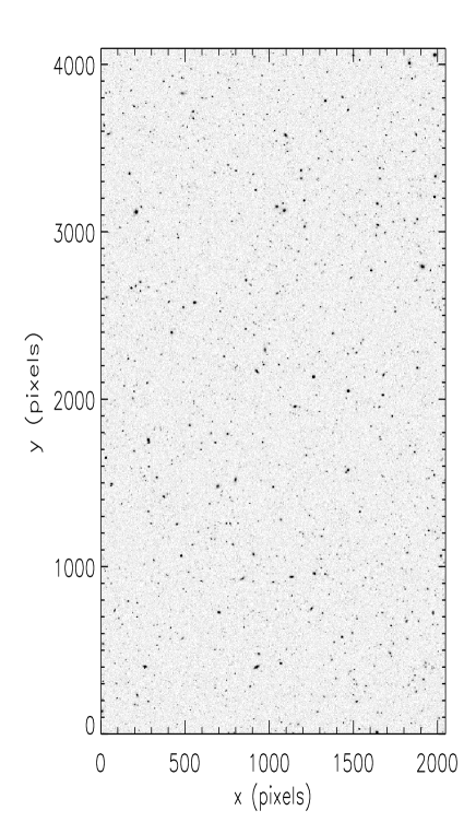
Figure 8: An example simulated image (see text for details).

Figure 9: The distribution of image magnitudes and half-light radii, $r_{h}$, for the data (top) and the simulation (bottom). These distributions are used for star/galaxy separation.

Figure 10: $\gamma^{{\rm in}}_{i}$ compared with $\gamma^{{\rm out}}_{i}$ for simulated data sheared (top) by 1.5% rms shear; (bottom) by 5% rms shear. The dashed line shows the $\gamma^{{\rm in}}_{i}=\gamma^{{\rm out}}_{i}$ relation; the solid line shows the best fit, $\gamma^{{\rm in}}_{i}=0.84\gamma^{{\rm out}}_{i}$.

8 Estimator for the Cosmic Shear

8.1 Shear Variance

The amplitude of the cosmic shear can be measured by considering the shear variance in excess of noise and systematic effects. In our experiment, we consider $N_{f}$ $8^{\prime}\times 16^{\prime}$ fields subdivided into $N_{c}=2N_{f}$ $8^{\prime}\times 8^{\prime}$ cells (see Figure 3). Let $\gamma^{fc}_{i}$ be the shear measured in cell $c$ of field $f$. Here, $c=t$ or $b$ for the top or bottom cells in each field, respectively. This shear is a sum of the contributions from lensing, noise and residual systematic effects, and can thus be written as

$$\gamma^{fc}_{i}=\gamma_{i}^{{\rm lens},fc}+\gamma_{i}^{{\rm noise},fc}+\gamma_{i}^{{\rm sys},fc}$$ (44)

We wish to measure the lensing shear variance $\sigma_{{\rm lens}}^{2}=\langle|\gamma^{{\rm lens},fc}|^{2}\rangle$ in excess of the noise variance $\sigma_{{\rm noise},fc}^{2}=\langle|\gamma^{{\rm noise},fc}|^{2}\rangle$ and systematic variance $\sigma_{{\rm sys,fc}}^{2}=\langle|\gamma^{{\rm sys},fc}|^{2}\rangle$. An estimator for the lensing variance is given by

$$\widehat{\sigma_{{\rm lens}}^{2}}\equiv\sigma_{{\rm tot}}^{2}-\sigma_{{\rm noise}}^{2}-\sigma_{{\rm sys}}^{2},$$ (45)

where the observed total variance is

$$\sigma_{{\rm tot}}^{2}\equiv\frac{1}{N_{c}}\sum_{f,c}|\gamma^{fc}|^{2},$$ (46)

and the mean noise and systematic variances are defined by

$$\sigma_{{\rm noise}}^{2}\equiv\frac{1}{N_{c}}\sum_{fc}\sigma_{{\rm noise},fc}^{2},~{}~{}~{}\sigma_{{\rm sys}}^{2}\equiv\frac{1}{N_{c}}\sum_{fc}\sigma_{{\rm sys},fc}^{2}.$$ (47)

It is easy to check that this estimator is unbiased, i.e. that

$$\langle\widehat{\sigma_{{\rm lens}}^{2}}\rangle=\sigma_{{\rm lens}}^{2},$$ (48)

where the brackets denote an ensemble average.

We can also compute the variance of $\widehat{\sigma_{{\rm lens}}^{2}}$ if we assume that the variables follow a gaussian distribution. This is a good approximation for $\gamma_{i}^{{\rm noise},fc}$, since we are considering an average over many galaxies (about 2000) in a cell. The systematic contribution to the shear is dominated by the residual anticorrelation discussed in §6.2 and thus has a distribution which is close to that of the stellar ellipticities. The stellar ellipticities are relatively well approximated by a gaussian distribution. In our case, it is therefore acceptable to take $\gamma_{i}^{{\rm sys},fc}$ to be gaussian. The lensing shear $\gamma_{i}^{{\rm lens},fc}$ is however known to be non-gaussian, especially on scales smaller than 10’ below which nonlinear density perturbations are dominant (e.g.. Jain & Seljak 1997; Gatzanaga & Bernardeau 1998). In principle, higher order correlation functions are required. These are however difficult to compute analytically on such small scales (Scoccimaro et al. 1999; Hui 1999), and are at the limit of the resolution of current N-body simulations (Jain et al. 1998; Barber et al. 1999; White et al. 1999).

We can now compute the variance of the estimator and find

$$\sigma^{2}[\widehat{\sigma_{{\rm lens}}^{2}}] = \frac{1}{N_{c}}\left[\left(\sigma_{lens}^{2}+\sigma_{noise}^{2}+\sigma_{sys}^{2}\right)^{2}+\right.$$ (49)

$$~{}~{}~{}\left.2\left(\sigma_{\times{\rm lens}1}^{4}+\sigma_{\times{\rm lens}2}^{4}\right)\right],$$

where $\sigma_{\times{\rm lens}i}^{2}$ are the cross-correlation variances between top and bottom cells due to lensing (see Eq. [19]). In deriving this expression, we have assumed that the noise and systematic effects are uncorrelated from the top to the bottom cell. We have also used the following approximation

$$\sigma_{{\rm noise}}^{2} \simeq \frac{1}{N_{f}}\sum_{f}\sigma_{{\rm noise},ft}^{2}\simeq\frac{1}{N_{f}}\sum_{c}\sigma_{{\rm noise},fb}^{2}$$ (50)

$$\simeq \left[\frac{1}{N_{c}}\sum_{f,c}\sigma_{{\rm noise},fc}^{4}\right]^{\frac{1}{2}}$$

This is valid given the cells were observed in very similar conditions, and thus the spread in the $\sigma_{{\rm noise},fc}^{2}$ is small.

Terms with a ‘lens’ subscript in equation (49) correspond to cosmic variance, while the other two terms correspond to the uncertainty produced by noise and systematic effects. If we are initially interested in a detection of cosmic shear, it suffices to test only the null hypothesis corresponding to the absence of lensing, i.e. to $\sigma_{{\rm lens}}=\sigma_{\times{\rm lens}i}=0$. The estimator variance relevant for a detection is

$$\sigma^{2}[\widehat{\sigma_{{\rm lens}}^{2}}]\simeq\frac{1}{N_{c}}\left[\sigma_{{\rm noise}}^{2}+\sigma_{{\rm sys}}^{2}\right]^{2}~{}~{}~{}{\rm(detection)}.$$ (51)

8.2 Shear Cross-Correlation

An important aspect of our experiment is our ability to test the the cross-correlation between the shear measured in 2 adjacent $8^{\prime}\times 8^{\prime}$ cells (see Figure 3). As before, let $\gamma^{ft}_{i}$ and $\gamma^{fb}_{i}$ be the average shear in the top and bottom portion of the $8^{\prime}\times 16^{\prime}$ field $f$, respectively. The shear cross-correlation variance (see Eq. [19]) is defined by

$$\sigma_{\times{\rm lens}}^{2}\equiv\langle\gamma^{ft}_{i}\gamma^{fb}_{i}\rangle,$$ (52)

where the summation convention is used. As before, we assume that the noise and systematic effects are uncorrelated across the two cells. An estimator for this quantity is then

$$\widehat{\sigma_{\times{\rm lens}}^{2}}\equiv\frac{1}{N_{f}}\sum_{f}\gamma_{i}^{ft}\gamma_{i}^{fb}.$$ (53)

It is again easy to check that it is unbiased, i.e. that

$$\langle\widehat{\sigma_{\times{\rm lens}}^{2}}\rangle=\sigma_{\times{\rm lens}}^{2}$$ (54)

Assuming as before that the fields are gaussian, we can compute the variance of this estimator and find

$$\sigma^{2}[\widehat{\sigma_{\times{\rm lens}}^{2}}] = \frac{1}{2N_{f}}\left[\left(\sigma_{lens}^{2}+\sigma_{noise}^{2}+\sigma_{sys}^{2}\right)^{2}+\right.$$ (55)

$$~{}~{}~{}\left.2\left(\sigma_{\times{\rm lens}1}^{4}+\sigma_{\times{\rm lens}2}^{4}\right)\right],$$

which equals $\sigma^{2}[\widehat{\sigma_{{\rm lens}}^{2}}]$. For a detection we must rule out the null hypothesis ($\sigma_{\times{\rm lens}1}^{2}=\sigma_{\times{\rm lens}2}^{2}=\sigma_{{\rm lens}}^{2}=0$). The relevant estimator variance for this purpose is then

$$\sigma^{2}[\widehat{\sigma_{\times{\rm lens}}^{2}}]=\frac{1}{2N_{f}}\left[\sigma_{noise}^{2}+\sigma_{sys}^{2}\right]^{2}~{}~{}~{}{\rm(detection)}.$$ (56)

9 Results

We now present and interpret our results, first using the simulations, and then examining the WHT data. The following description is summarised in Table 3 for convenience.

9.1 Simulated Fields

We begin with the null simulations, which consists of 20 8’$\times$8’ disjoint cells. The distribution of the shear for each simulated cell is shown on figure 11.

For the null simulation, the rms noise (Eq. [47]) is $\sigma_{{\rm noise}}\simeq 0.0103$, while the observed total rms is $\sigma_{{\rm total}}\simeq 0.0113$ (Eq. [46]) . The noise and total rms are indicated as a solid and dashed line in figure 11, respectively. Clearly, in the absence of a lensing signal, $\sigma_{{\rm sys}}^{2}=\sigma_{{\rm total}}^{2}-\sigma_{{\rm noise}}^{2}$, which gives $\sigma_{{\rm sys}}\simeq 0.0047$.

We also require the error for $\sigma_{{\rm sys}}$. In a fashion similar to that of equation(51), we find that

$$\sigma^{2}[\widehat{\sigma_{{\rm sys}}^{2}}]\simeq\frac{1}{N_{c}}\left[\sigma_{{\rm noise}}^{2}+\sigma_{{\rm sys}}^{2}\right]^{2}$$ (57)

giving $\sigma[\widehat{\sigma_{{\rm sys}}^{2}}]\simeq(0.0053)^{2}$, so that $\sigma^{2}_{{\rm sys}}=(0.0047)^{2}\pm(0.0053)^{2}$. Note that this is consistent with zero; i.e. even if we supposed that there were no systematics, the excess shear signal that we would attribute to real lensing would be consistent with zero.

We can check this result against our next simulation, which now includes a 1.5% rms shear in 30 8’$\times$8’ cells. We can first use this simulation to derive an independent constraint on $\sigma_{{\rm sys}}$.

$$\widehat{\sigma_{{\rm sys}}^{2}}=\sigma_{{\rm total}}^{2}-\sigma_{{\rm noise}}^{2}-\sigma_{{\rm lens}}^{2}$$ (58)

where we let $\sigma_{{\rm lens}}=0.015$ i.e. the input rms shear.

For this simulation, we find $\sigma_{{\rm noise}}\simeq 0.0130$, $\sigma_{{\rm total}}\simeq 0.0193$ (see figure 12). The error for $\sigma_{{\rm sys}}$ this time is computed as follows

$$\sigma^{2}[\widehat{\sigma_{{\rm sys}}^{2}}]\simeq\frac{1}{N_{c}}\left[\sigma_{{\rm noise}}^{2}+\sigma_{{\rm sys}}^{2}+\sigma_{{\rm lens}}^{2}\right]^{2}.$$ (59)

However, since $\sigma_{{\rm total}}^{2}-\sigma_{{\rm noise}}^{2}<0.015^{2}$, we can only find an upper limit for $\sigma_{\rm sys}$ here; we find that $\sigma[\sigma_{{\rm sys}}^{2}]=\pm(0.0082)^{2}$, consistent with the null simulation result. Accordingly, in what follows, we will use the null simulation estimate for $\sigma^{2}_{{\rm sys}}$.

Turning this around, we can use equation (45) to estimate the rms shear in these simulations (ignoring our knowledge of the input rms shear). We obtain (using the null simulation estimate of $\sigma_{\rm sys}$) $\sigma_{\rm lens}\simeq 0.013$. The uncertainty in $\sigma_{\rm lens}^{2}$ is calculated using equation (51) for detection and equation (49) for measurement. We obtain $\sigma[\sigma_{\rm lens}^{2}]=(0.0060)^{2}$ for detection, and $\sigma[\sigma_{\rm lens}^{2}]=(0.0082)^{2}$ for measurement. Notice that this is the same value as $\sigma[\sigma_{\rm sys}^{2}]$, since we can’t independently find $\sigma_{\rm sys}$ and $\sigma_{\rm lens}$ for the simulations. The measured rms shear is thus fully consistent with the input rms shear of 1.5% (Figure 12).

An analogous analysis is done for the 5% rms shear simulations; see table 3. Again, we recover the input rms shear within the uncertainties. Note again that, since $\sigma_{{\rm total}}^{2}-\sigma_{{\rm noise}}^{2}<0.05^{2}$, only an upper limit can be found for $\sigma_{\rm sys}$ here. We can conclude that the simulations clearly show that in the relevant regimes, our method is unbiased.

9.2 Observed fields

We now consider the observed fields. The distribution of shear for each of the 26 cells is plotted on figure 13, along with circles corresponding to $\sigma_{{\rm noise}}$ and $\sigma_{{\rm tot}}$. The mean shear components are $\overline{\gamma}_{1}=-0.00097\pm 0.0034$ , $\overline{\gamma}_{2}=0.0021\pm 0.0034$ , fully consistent with zero as they should be in the absence of systematic effects. What is more, we are measuring a total shear variance in excess of the noise. We now determine whether this detection is significant.

The value for the rms noise is $\sigma_{{\rm noise}}=0.018$, somewhat larger than in our simulations. This is due to increased noise from stellar ellipticity fitting and, in poorer seeing cases, lower number density. The total rms shear is $\sigma_{{\rm tot}}=0.024$, and using $\sigma_{{\rm sys}}=0.0047$ from the null simulations, we obtain $\sigma_{{\rm lens}}=0.0156$ (from Eq. [45]).

Table 3: Shear measurement results for the simulated and WHT fields

	Sim.	Sim.	Sim.	Data
	Null	1.5%	5%
$N_{c}$	20	30	20	26
$\sigma_{{\rm tot}}^{2}$	$(0.0113)^{2}$	$(0.0193)^{2}$	$(0.0494)^{2}$	$(0.0243)^{2}$
$\sigma_{{\rm noise}}^{2}$	$(0.0103)^{2}$	$(0.0130)^{2}$	$(0.0102)^{2}$	$(0.0179)^{2}$
$\sigma_{{\rm sys}}^{2}$	$(0.0047)^{2}\;{}^{a}$	$0\;^{c}$	$0\;^{d}$	$(0.0047)^{2}\;{}^{e}$
$\sigma_{{\rm lens}}^{2}$	$(0.0047)^{2}\;{}^{b}$	$(0.0132)^{2}$	$(0.0480)^{2}$	$(0.0156)^{2}$
$\sigma_{\times{\rm lens}}^{2}$				$(0.0156)^{2}$
$\sigma[\sigma_{{\rm sys}}^{2}]$	$(0.0053)^{2}\;{}^{a}$	$(0.0082)^{2}$	$(0.0234)^{2}$	$(0.0053)^{2}$
$\sigma[\sigma_{{\rm lens}}^{2}]$ (detect)	$(0.0053)^{2}$	$(0.0060)^{2}$	$(0.0055)^{2}$	$(0.0082)^{2}$
$\sigma[\sigma_{{\rm lens}}^{2}]$ (measure)	$(0.0053)^{2}\;{}^{b}$	$(0.0082)^{2}$	$(0.0234)^{2}$	$(0.0119)^{2}$

^a assumes $\sigma_{{\rm lens}}$=0.
^b assumes $\sigma_{{\rm sys}}$=0.
^c assumes $\sigma_{{\rm lens}}$=0.015
^d assumes $\sigma_{{\rm lens}}$=0.05
^e Uses the null simulation value, since we can not obtain an independent estimate

Using equation (51), we find the error in $\sigma_{{\rm lens}}$ to be $\sigma[\widehat{\sigma_{{\rm lens}}^{2}}]\simeq(0.0082)^{2}$ for the statistical error only. If we also include the uncertainty on the systematic (by adding it in quadrature), we obtain $\sigma[\widehat{\sigma_{{\rm lens}}^{2}}]\simeq(0.0084)^{2}$. We therefore quote our result as

$$\sigma_{{\rm lens}}^{2} = \sigma_{{\rm lens,measured}}^{2}\pm\sigma[\widehat{\sigma_{{\rm lens}}^{2}}]_{{\rm statistical}}\pm\sigma[\widehat{\sigma_{{\rm sys}}^{2}}]$$ (60)

$$= (0.0156)^{2}\pm(0.0082)^{2}\pm(0.0047)^{2}.$$

The significance of our detection of the cosmic shear is therefore

$$(S/N)_{{\rm detect}}=\frac{\sigma_{{\rm lens}}^{2}}{\sigma[\widehat{\sigma_{{\rm lens}}^{2}}]_{{\rm total}}}\simeq 3.4$$ (61)

In terms of measuring the amplitude of the cosmic shear, we use equation (49) and find $\sigma[\sigma_{\rm lens}^{2}]=(0.0119)^{2}$; including the uncertainty on the systematic we obtain $\sigma[\sigma_{\rm lens}^{2}]=(0.0121)^{2}$. We therefore find

$$\sigma_{{\rm lens}}^{2} = \sigma_{{\rm lens,measured}}^{2}\pm\sigma[\widehat{\sigma_{{\rm lens}}^{2}}]_{{\rm statistical}}\pm\sigma[\widehat{\sigma_{{\rm sys}}^{2}}]$$ (62)

$$= (0.0156)^{2}\pm(0.0119)^{2}\pm(0.0057)^{2},$$

where we have included in $\sigma_{{\rm sys}}$ the uncertainty in our KSB shear calibration (see section 7). Thus we find that $(S/N)_{{\rm measure}}\simeq 1.7$.

The final measurement we can make is the cross-correlation covariance using equation (53). We find that $\sigma_{\times 1}\simeq 0.0115$, $\sigma_{\times 2}\simeq 0.0105$, leading to $\sigma_{\times}$ = 0.0156. For a detection, $\sigma[\sigma_{\times}^{2}]\simeq(0.0088)^{2}$ (Eq. [56]), so that the significance of the detection is $(S/N)_{{\rm detect}}\simeq 3.2$ for the cross-correlation. For a measurement, $\sigma[\sigma_{\times}^{2}]\simeq(0.0119)^{2}$ (Eq. [55]), so $(S/N)_{{\rm measure}}\simeq 1.7$.

Figure 11: Mean $\gamma_{1}$ and $\gamma_{2}$ for 20 simulated null cells. The dashed circle shows the noise rms, the solid circle shows the total rms. The difference is consistent with zero signal.

Figure 12: Mean $\gamma_{1}$ and $\gamma_{2}$ for 30 simulated cells with rms 1.5% shear. The dashed circle shows the noise rms, the solid circle shows the total rms.

Figure 13: Mean $\gamma_{1}$ and $\gamma_{2}$ for the observed cells. The dashed circle shows the noise rms, the solid circle shows the total rms.

9.3 Cosmological Implications

A key question we must now address is the redshift distribution of our background sources. At the median magnitude of the original catalogue ($R$=25.2$\pm$0.2, Table 2, $\S$3.2), photometric redshift estimators in various HST and ground-based datasets suggest a mean redshift $z\simeq$1-1.2 (Fernandez-Soto et al 1999, Poli et al 1999, Rhodes 1999). More importantly, for the survey sample, which is effectively limited at a median magnitude of $R\simeq 23.4\pm$0.2, we make use of the recently-completed deep spectroscopic survey of Cohen et al (2000) which indicates a median redshift at this limit $z$=0.8$\pm$0.2; the uncertainty here includes the observed field-to-field variations in this limiting depth as in Table 2.

We can now compare these results with those predicted for the various cosmological models listed in Table 1. First, we compare our value of $\sigma_{\rm lens}^{2}=(0.016)^{2}\pm(0.012)^{2}$ (with errors which includes cosmic variance). We find that our result is consistent with the cluster normalised models $\tau$CDM, $\Lambda$CDM and OCDM at the 0.6-0.9 $\sigma$ level, but that it is inconsistent with the COBE normalised SCDM model at the 3.0$\sigma$ level. This confirms the fact that the SCDM model has too much power on small scales when normalised to COBE.

The cross-correlation variance $\sigma_{\times{\rm lens}}^{2}=(0.0156)^{2}\pm(0.0119)^{2}$ (again with cosmic variance included in the uncertainty) does not provide as strong a constraint. It is consistent with the models, with deviations of between 0.1$\sigma$ to 1.4$\sigma$. This results from the fact that $\sigma_{\times{\rm lens}}^{2}$ is expected to have a smaller amplitude than $\sigma_{{\rm lens}}^{2}$ in all models. It is nevertheless comforting that, within the context of the models considered, it is consistent with our measurement of $\sigma_{{\rm lens}}^{2}$.

We can use our measurement of $\sigma_{{\rm lens}}^{2}$ to constrain $\sigma_{8}$, the normalisation of the matter power spectrum on 8 $h^{-1}$ Mpc scales. For the $\Lambda$CDM model with $\Omega_{m}=0.3$, we find from equation (20) that these two quantities are related by

$$\sigma_{8}=0.894z_{s}^{-0.648}\left(\frac{\sigma_{\rm lens}}{0.01}\right)^{0.8}$$ (63)

For our value of $\sigma_{\rm lens}$ and setting $z_{s}=0.8\pm 0.2$ (see §3.2) and propagating errors, this yields

$$\sigma_{8}=1.47\pm 0.24\pm 0.46=1.47\pm 0.51,$$ (64)

where the first error arises from the uncertainty in $z_{s}$ and the second from that of $\sigma_{\rm lens}^{2}$. This corresponds to a 2.9$\sigma$ measurement of $\sigma_{8}$. We can compare this with the cluster abundance determination which yield $\sigma_{8}=(0.6\pm 0.1)\Omega_{m}^{-0.53}=(1.13\pm 0.19)\left(\frac{\Omega_{m}}{0.3}\right)^{-0.53}$. We see that our result is consistent with this independent determination. Note that the uncertainty in $z_{s}$ does not dominate our uncertainty for $\sigma_{8}$.

10 Conclusions

Using 14 $8^{\prime}\times 16^{\prime}$ fields observed homogeneously with the WHT, we have detected a shear signal arising from weak lensing by large scale structure. Neglecting cosmic variance (to test the null hypothesis corresponding to the absence of lensing), we find a shear variance in $8^{\prime}\times 8^{\prime}$ cells of $(0.016)^{2}\pm(0.008)^{2}\pm(0.005)^{2}$, where the errors correspond to $1\sigma$ statistical and systematic uncertainties, respectively. This corresponds to a detection significant at the $3.4\sigma$ level. Including (gaussian) cosmic variance, the shear variance is $(0.016)^{2}\pm(0.012)^{2}$. This is consistent with the value expected for cluster-normalised CDM models ($\sigma_{\rm lens}=(1.0-1.3)\times 10^{-2}$). On the other hand, the COBE-normalised SCDM model is rejected at the ($3.0\sigma$) level. We have verified our results by measuring the cross-correlation of the shear in adjacent cells. We find that the resulting cross-correlation variance for detection is $(0.016)^{2}\pm(0.009)^{2}$, and for measurement is $(0.016)^{2}\pm(0.012)^{2}$, in agreement with that expected in cluster normalised CDM models. This is consistent with all the models considered at the $1\sigma$ level.

Our measurement was derived after a careful accounting of the systematic effects which can produce a spurious shear signal. We find that the most serious systematic effect is the PSF overcorrection for faint objects in the shear measurement method. We have shown however that, by keeping only sufficiently bright objects ($S/N>15$), this effect can be made to be smaller than the statistical uncertainty. Our methods have been tested using detailed numerical simulations of the shear signal from appropriately-constructed synthetic sheared images. We find very good statistical agreement between the simulated and the observed data. An extensive description of the simulations will be described in Bacon et al. (2000).

For a given cosmological model, our measurement can be turned into a measurement of $\sigma_{8}$, the normalisation of the mass power spectrum on 8 $h^{-1}$ Mpc scales. For a $\Lambda$CDM model with $\Omega_{m}=0.3$, we get $\sigma_{8}=1.5\pm 0.2\pm 0.5$, where the errors are $1\sigma$ uncertainties resulting from the uncertainty in the redshift of the background galaxies and from our measurement error, respectively. This result is consistent with the $\sigma_{8}$ value derived from cluster abundance ($\sigma_{8}=(1.13\pm 0.19)\left(\frac{\Omega_{m}}{0.3}\right)^{-0.53}$, Viana & Liddle 1996).

The uncertainty in our measurement is clearly dominated by cosmic variance and statistical errors. This can be improved by increasing the number of fields $N_{f}$. Since the signal-to-noise ratio scales as $\sqrt{N_{f}}$, a four fold improvement in $N_{f}$ should yield a $6.8\sigma$ detection and a $3.4\sigma$ measurement of the rms shear. This, and the presence of other wide field cameras, offers good prospects for the improvement of the measurement of $\sigma_{8}$ from cosmic shear. On the other hand the determination of $\sigma_{8}$ from cluster abundance is currently measured only at the $~{}6\sigma$ level and is fundamentally limited by the finite number of nearby clusters, for which accurate temperatures can be determined. In addition, it depends sensitively on the assumption of gaussian initial conditions. It is therefore likely that cosmic shear measurements will supplant cluster abundance for the normalisation of the power spectrum. With an even larger number of fields, one can also measure the shape of the power spectrum by looking at the correlation of the shear between and within nearby fields. The advent of wide-field cameras will make this possible in the near future.

References

- [1] Barber A. J., Thomas P. A., Couchman H. M. P., 1999, MNRAS, 310, 453
- [2] Bardeen J. M., Bond J. R., Kaiser N., Szalay A. S., 1986, ApJ, 304, 15
- [3] Bartelmann M., Schneider P., 1999, submitted to Physics Reports, preprint astro-ph/9912508
- [4] Baugh C., Cole S., Frenk C. S., Lacey C. G., 1998, ApJ, 498, 504
- [5] Bacon D., Refregier A., Clowe D., Ellis R., 2000, preprint astro-ph/0007023
- [6] Bertin E., Arnoults S., 1996, A&AS, 117, 393
- [7] Blandford R. D., Saust A. B., Brainerd T. G., Villumsen J. V., 1991, MNRAS, 251, 600
- [8] Carter D., Bridges T., 1995, WHT Prime Focus and Auxiliary Port Imaging Manual, available at http:// lpss1.ing.iac.es/ manuals/html_manuals/wht_instr/pfip
- [9] Bonnet H., Mellier Y., Fort B., 1994, ApJ, 427, L83
- [10] Bunn E. F., White M., 1997, ApJ, 480, 6
- [11] Ebbels T., 1998, Ph.D. thesis, University of Cambridge
- [12] Fernandez-Soto A., Lanzetta K. M., Yahil A., 1999, ApJ, 513, 34
- [13] Fort B., Mellier Y., 1994, Astron. Astr. Rev., 5, 239
- [14] Fort B., Mellier Y., Dantel-Fort M., Bonnet H., Kneib J.-P., 1996, A&A, 310, 705
- [15] Gaztanaga E., Bernardeau F., 1998, A&A, 331, 829
- [16] Groth et al., 1998, BAAS
- [17] Hu W., Tegmark M., 1998 (astro-ph/9811168)
- [18] Hui L., 1999, submitted to ApJL, preprint astro-ph/9902275
- [19] Jain B., Seljak U., 1997, ApJ, 484, 560
- [20] Jain B., Seljak U., White S., 1998 (astro-ph/9804238)
- [21] Jungman G., Kamionkowski M., Kosowsky A., Spergel D. N., 1996, PRD, 54, 1332
- [22] Kaiser N., 1992, ApJ, 388, 272
- [23] Kaiser N., 1998a, ApJ, 498, 26
- [24] Kaiser N., Wilson G., Luppino G., Kofman L., Gioia I., Metzger M., Dahle H., submitted to ApJ, preprint astro-ph/9809268
- [25] Kaiser N., Squires G., Broadhurst T., 1995, ApJ, 449, 460
- [26] Kaiser N., 1999a, Review talk for Boston 99 lensing meeting, preprint astro-ph/9912569
- [27] Kaiser N., 1999b, preprint astro-ph/9904003
- [28] Kuijken K., 1999, submitted to A&A, preprint astro-ph/9904418
- [29] Kamionkoski M., Babul A. Cress C. M., Refregier A., 1997, MNRAS, 301, 1064, preprint astro-ph/9712030
- [30] Kauffmann G., Guiderdoni B., White S. D. M., 1994, MNRAS, 267, 981
- [31] Mellier Y., van Waerbeke L., Bernardeau F., Fort B., 1996 (astro-ph/9609197)
- [32] Mellier Y., 1999, ARAA, 37, 127
- [33] Mould J., Blandford R., Villumsen J., Brainerd T., Smail I., Smail I., Kells W., 1994, MNRAS, 271, 31
- [34] Peacock J., Dodds S. J., 1997, MNRAS, 280, L19
- [35] Poli F., Giallongo E., Menci N., D’Odorico S., Fontana A., 1999, ApJ, 527, 662
- [36] Refregier A., Brown S. T., Kamionkowski M., Helfand D. J., Cress C. M., Babul A., Becker R., White R. L., 1998, in Procs. of XIVth IAP meeting, Wide Field Surveys in Cosmology, Eds. Mellier Y. & Colombi S., preprint astro-ph/9810025
- [37] Rhodes J., 1999, PhD thesis, Department of Physics, Princeton University
- [38] Rhodes J., Refregier A., Groth E., 1999, to appear in ApJ, preprint astro-ph/9505090
- [39] Schneider P., van Waerbeke L., Jain B., Kruse G., 1998a, MNRAS, 296, 873
- [40] Schneider P., van Waerbeke L., Mellier Y., Jain B., Seitz S., Fort B., 1998b, A&A, 333, 767
- [41] Schneider P., 1996 in Universe at High Z, eds. Martinez-Gonzalez & Sanz, p470
- [42] Scoccimarro R., Zaldarriaga M., Hui L., 1999, ApJ, 527, 1
- [43] Seitz S. et al. 1998, in Procs. of XIVth IAP meeting, Wide Field Surveys in Cosmology, Eds. Mellier, Y. & Colombi, S.
- [44] Smail I., Hogg D., Lin Y., Cohen J., 1995, ApJ, 449, L105
- [45] Smail I., Ellis R. S., Dressler A., Couch W. J., Oemler A., Sharples R. M., Butcher H., 1997, ApJ, 479, 70
- [46] van Waerbeke L., Bernardeau F., Mellier Y., 1999, A&A in press, astro-ph/9807007
- [47] Villumsen J., 1995 (astro-ph/9507007)
- [48] Viana P., Liddle A., 1996, MNRAS, 281, 323
- [49] White M., Hu W., 1999, preprint astro-ph/9909165