Weak gravitational lensing: reducing the contamination by intrinsic alignments

Abstract

Intrinsic alignments of galaxies can mimic to an extent the effects of shear caused by weak gravitational lensing. Previous studies have shown that for shallow surveys with median redshifts $z_{m}\sim 0.1$, the intrinsic alignment dominates the lensing signal. For deep surveys with $z_{m}\sim 1$, intrinsic alignments are believed to be a significant contaminant of the lensing signal, preventing high-precision measurements of the matter power spectrum. In this paper we show how distance information, either spectroscopic or photometric redshifts, can be used to down-weight nearby pairs in an optimised way, to reduce the errors in the shear signal arising from intrinsic alignments. Provided a conservatively large intrinsic alignment is assumed, the optimised weights will essentially remove all traces of contamination. For the Sloan spectroscopic galaxy sample, residual shot noise continues to render it unsuitable for weak lensing studies. However, a dramatic improvement for the slightly deeper Sloan photometric survey is found, whereby the intrinsic contribution, at angular scales greater than 1 arcminute, is reduced from about 80 times the lensing signal to a 10% effect. For deeper surveys such as the COMBO-17 survey with $z_{m}\sim 0.6$, the optimisation reduces the error from a largely systematic $\sim 220$% error at small angular scales to a much smaller and largely statistical error of only 17% of the expected lensing signal. We therefore propose that future weak lensing surveys be accompanied by the acquisition of photometric redshifts, in order to remove fully the unknown intrinsic alignment errors from weak lensing detections.

Weak gravitational lensing: reducing the contamination by intrinsic alignments

1 Introduction

Weak gravitational lensing by intervening large-scale structure introduces a coherent distortion in faint galaxy images. Several independent surveys have measured this ‘cosmic shear’ effect and are now able estimate the bias parameter, b, (?; ?) and set joint constraints on the values of the matter density parameter $\Omega_{\rm m}$ and the amplitude of the matter power spectrum, $\sigma_{8}$ (?; ?; ?; ?; ?; ?).

A potential limitation of this technique is the intrinsic correlation of the ellipticities of nearby galaxies which can result from gravitational interactions during galaxy formation. This ‘tidal torquing’ leads to a net alignment of nearby galaxies which could produce a spurious signal similar to that induced by weak gravitational lensing. A number of studies have investigated the amplitude of this intrinsic alignment effect with some broad agreement, (?, hereafter HRH, ?; ?; ?; ?; ?; ?; ?; ?), but it is fair to say that an accurate estimate of this effect eludes us. For low-redshift surveys, for example SuperCOSMOS and the Sloan spectroscopic galaxy sample, where the median redshift is $z_{m}\sim 0.1$, the correlation of ellipticities due to intrinsic alignment is far greater than the expected lensing signal. As the survey depth increases, galaxies at fixed angular separation are distributed over wider ranges of redshifts, leaving only a small proportion of the galaxy pairs close enough for tidal interactions to correlate the ellipticities. This reduction in the total angular intrinsic alignment signal, combined with an increasing line-of-sight distance boosting the lensing signal, leaves a smaller intrinsic alignment contamination for deeper surveys. The majority of studies find that for surveys with depths $z_{m}\sim 1$ the estimated contamination contributes to up to $\sim 10\%$ of the lensing signal, although ? has argued that the contamination could be much higher. As cosmic shear measurements become more accurate these low levels of contamination cannot be considered negligible.

If an accurate estimate of the intrinsic ellipticity correlation strength did exist, then it would be possible to subtract it, leaving the correlation induced purely by lensing. In the absence of a good estimate for the intrinsic correlation function, it is obvious that one can improve upon a straightforward ellipticity correlation by down-weighting galaxy pairs close in redshift and angular sky separation. This can be done at the expense of increasing the shot noise contribution from the distribution of individual galaxy ellipticities.

In this work, we deduce the optimal pair weighting for an arbitrary survey, given accurate information about the galaxy distances. We use these results on the Sloan spectroscopic survey design to show that the optimal weighting scheme can largely remove the contamination by intrinsic alignments leaving almost pure shot noise. The shallow depth of this spectroscopic sample still prevents its use for weak lensing studies as the remaining shot noise exceeds the expected weak lensing signal.

For multi-colour surveys with photometric redshift information we propose a semi-optimised procedure of excluding pairs which are likely to be close in three dimensions. Comparison with the optimal method shows this can be very effective. We apply this technique to the Sloan photometric survey (SDSS) with $z_{m}\sim 0.2$, and three deeper surveys, the Red-Sequence Cluster Survey (RCS) with $z_{m}\sim 0.56$, (?), a sample of the COMBO-17 survey with $z_{m}\sim 0.6$, (?) and the Oxford Dartmouth Thirty survey (ODT) with $z_{m}\sim 1.0$, (?). We find that even with fairly inaccurate photometric redshifts it is possible to reduce the contamination from intrinsic alignments significantly. For the photometric SDSS, the improvement is dramatic, enabling it to be used as a weak lensing survey. For the deeper surveys we show that using this weighting scheme, intrinsic alignment contamination can be reduced by several orders of magnitude.

The effect of the non-uniform weighting on the weak lensing shear correlation function is calculated. We find that galaxy pair weighting slightly reduces the lensing signal, the reduction dependent on the photometric redshift accuracy and the survey depth.

This paper is organised as follows. In $\S$2 we briefly describe related weak lensing theory. In §3 we derive the optimal pair weighting for a spectroscopic survey. We discuss the results of pair weighting for the Sloan spectroscopic sample in $\S$4, comparing HRH and Jing intrinsic alignment models. In $\S$5 we propose an alternative scheme for multi-colour surveys with photometric redshift information and present the results in $\S$6. These results are compared with the expected weighted lensing signal derived in the Appendix. In $\S$7 we discuss the results and the implications for the design of future weak lensing surveys.

2 Theory

In the weak lensing limit the ellipticity of a galaxy, $(e_{1},e_{2})$, is an unbiased estimate of the shear $\gamma$, the stretching and compression of the galaxy image caused by the gravitational lensing of its light. Ellipticity is defined by approximating each galaxy as an ellipse with axial ratio $\beta$, at position angle $\phi$, measured counterclockwise from the x-axis.

$$\left(\begin{array}[]{c}e_{1}\\ e_{2}\end{array}\right)=\frac{\beta^{2}-1}{\beta^{2}+1}\left(\begin{array}[]{c}\cos 2\phi\\ \sin 2\phi\end{array}\right)$$ (1)

The complex shear $\gamma$ is related to the average galaxy ellipticity by $\gamma\simeq\langle e\rangle/2\equiv\langle e_{1}+ie_{2}\rangle/2$. A useful statistic which can be used to constrain the matter power spectrum is the shear correlation function, $\langle\gamma\gamma^{*}\rangle_{\theta}$, for galaxies separated by angle $\theta$. For randomly-orientated galaxies in the absence of weak lensing, a correlation of galaxy ellipticities would yield a zero result at all angular scales. The presence of weak lensing introduces coherent shearing distortions, producing ellipticity or shear correlations which are related to the nonlinear mass power spectrum $P_{\delta}$ via

$$\langle\gamma\gamma^{*}\rangle_{\theta}=\frac{1}{2\pi}\int dk\,k\,P_{\kappa}(k)\,J_{0}(k\theta),$$ (2)

where $J_{0}$ is the zeroth Bessel function of the first order and $P_{\kappa}(k)$ is the convergence power spectrum at wave number $k$,

$$P_{\kappa}(k)=\frac{9H_{0}^{4}\Omega_{m}^{2}}{4c^{4}}\int_{0}^{w_{H}}dw\,\frac{g^{2}(w)}{a^{2}(w)}\,P_{\delta}\left(\frac{k}{f_{K}(w)},w\right),$$ (3)

$f_{K}(w)$ is the comoving angular diameter distance out to a comoving radial geodesic distance $w$, and is defined in the Appendix; $a(w)$ is the dimensionless scale factor, $H_{0}$ is the Hubble parameter and $\Omega_{m}$ the matter density parameter. The second argument of $P_{\delta}$ allows for time-evolution of the power spectrum. $g(w)$ is a weighting function locating the lensed sources,

$$g(w)=\int_{w}^{w_{H}}\,dw^{\prime}\ \phi(w^{\prime})\frac{f_{K}(w^{\prime}-w)}{f_{K}(w^{\prime})}.$$ (4)

$\phi(w(z))$ is the redshift distribution or selection function, and $w_{H}$ is the horizon distance, (?).

In addition to shear correlations produced by lensing, several groups have found evidence for an intrinsic alignment component. This means that to some degree, galaxies are not randomly orientated. In the absence of intrinsic correlations, the shear correlation function $\langle\gamma\gamma^{*}\rangle_{\theta}$ can be estimated from a catalogue of galaxy shapes through estimates of the ellipticity correlation function

$$\widehat{\langle e_{a}e_{b}^{*}\rangle}_{\theta}=Real\left[\frac{\sum_{ab}W_{ab}\,{\rm e}_{a}({\bf x})\,{\rm e}_{b}^{*}({\bf x}+\mbox{\boldmath{$\theta$}})}{\sum_{ab}W_{ab}}\right]$$ (5)

where $e_{a}$ is the ellipticity of galaxy $a$. In practice the pair sum is taken over galaxies in a small range $\Delta\theta$.

Typically the weight assigned to each pair of galaxies, $W_{ab}$, is the product of the uncertainty in each galaxy shape measurement. In the next section we derive an additional optimal pair weight which, in effect, down-weights galaxy pairs close enough to contribute to a contaminating intrinsic alignment signal, enabling the ellipticity correlation estimator to be directly related to the lensing shear correlation function.

3 Optimal Pair Weighting for Spectroscopic Surveys

The ellipticity correlation function, for pairs separated by an angle $\theta$ is given by equation 5. This estimate includes an uncertain contribution from intrinsic alignments, $I_{ab}$. The estimate of the lensing shear correlation function $E[\gamma\gamma^{*};\theta]$ is therefore

$$E[\gamma\gamma^{*};\theta]=\frac{1}{4}{\sum_{ab}W_{ab}\left(e_{a}e_{b}^{*}-I_{ab}\right)\over\sum_{ab}W_{ab}}$$ (6)

The amplitude of the intrinsic correlation is controlled by the comoving distance between the galaxy pair. It is only significant for galaxies closer than a few tens of Mpc at most, in which case the comoving separation is given by

$$R_{ab}^{2}\simeq(w_{a}-w_{b})^{2}+\left[f_{K}\left({w_{a}+w_{b}\over 2}\right)\right]^{2}\theta^{2}.$$ (7)

In principle, the intrinsic ellipticity correlation depends on the orientation of the galaxy pair in three dimensions, and also on the redshifts of the galaxies. However, studies of the intrinsic effect average over the orientation, and there seems to be little evolution with redshift. Thus we assume we have an estimate of an average correlation function which depends only on the separation $R$ of the two galaxies:

$$\eta_{I}(R)\equiv\langle e({\bf x})e^{*}({\bf x}+{\bf R})\rangle_{I}.$$ (8)

where the average is over galaxy positions ${\bf x}$, assumed to be known precisely. In practice, peculiar velocity distortions and spectroscopic redshift uncertainties lead to errors of order $\Delta z\sim 0.001$, which we will neglect. This is justified because, as we show in section 6, surveys with photometric redshift errors much larger than this can have intrinsic signals removed virtually as effectively as the idealised example treated here. $\eta_{I}(R)$ can be calculated approximately, from numerical simulations (HRH, ?; ?) or analytic approximation (?; ?; ?; ?; ?). The published results do differ by more than an order of magnitude, and this uncertainty has to be considered when choosing which $\eta_{I}(R)$ model to use in the following pair weighting scheme. The preferred strategy when applying this technique is to assume the largest theoretical model for $\eta_{I}(R)$ to ensure that all feasible contamination from intrinsic alignments is removed. This is discussed further in section 6.

To calculate the angular intrinsic contribution to the weak lensing signal, $\eta_{I}(R)$ is averaged over galaxy pairs separated by $\theta$ with a redshift distribution characteristic of the depth of the survey. This can be compared to the signal measured from low-redshift surveys such as the SuperCOSMOS survey (?), where ellipticity correlations are dominated by intrinsic alignments. These studies show very rough agreement of the amplitude of the effect, but the problem is sufficiently difficult that a definitive accurate study has yet to emerge. To quantify our uncertainty on the intrinsic correlations, we assume the intrinsic alignment prediction has a fractional error $f$ and thus a variance

$$\sigma_{IA}^{2}=f^{2}\langle I_{ab}\rangle^{2}$$ (9)

where $\langle I_{ab}\rangle$ is a weighted average. and we will conservatively take $f\simeq 1$ in what follows. The error in the estimator of the lensing correlation function, equation 6, has two main sources: uncertainty in the intrinsic correction, and shot noise from the intrinsic ellipticity distribution. If the variance of Real($e_{a}e_{b}^{*}$) is $\sigma_{\rm pair}^{2}$, then the shot noise error is

$$\sigma_{\rm SN}^{2}={\sum_{ab}W_{ab}^{2}\sigma_{\rm pair}^{2}\over\left(\sum_{ab}W_{ab}\right)^{2}}.$$ (10)

In the limit of an infinite number of galaxies, $\sigma_{\rm SN}$ tends to zero.

Considering the shot noise error and intrinsic alignment error only, the total error on the lensing correlation function is then given by

$$\sigma_{L}^{2}={\sum_{ab}W_{ab}^{2}\sigma_{\rm pair}^{2}+\left(\sum_{ab}W_{ab}fI_{ab}\right)^{2}\over\left(\sum_{ab}W_{ab}\right)^{2}}$$ (11)

We minimise this variance subject to $\sum_{ab}W_{ab}=$ constant. The weights for a galaxy pair $p=\{a,b\}$ then satisfy

$$W_{p}\sigma_{\rm pair}^{2}+f^{2}I_{p}\sum_{q}W_{q}I_{q}={\lambda^{\prime}\over 2}$$ (12)

where $\lambda^{\prime}$ is a Lagrange multiplier. If we define a matrix

$$M_{pq}\equiv J_{p}J_{q}$$ (13)

where

$$J_{p}\equiv{fI_{p}\over\sigma_{\rm pair}}$$ (14)

then $W_{p}$ satisfies

$$W_{p}+M_{pq}W_{q}=\lambda U_{p}$$ (15)

where $\lambda$ is an unimportant constant which we will set later by choosing the weights of uncorrelated pairs ($J_{p}$=0) to be unity. $U_{p}$ is a ‘unit’ vector consisting entirely of ones. The solution is

$${\bf W}=({\bf I}+{\bf M})^{-1}{\bf U}.$$ (16)

Because of the form of M, the inverse can be computed, by expanding $({\bf I}+{\bf M})^{-1}={\bf I}-{\bf M}+{\bf M}^{2}-\ldots$, with elements $[({\bf I}+{\bf M})^{-1}]_{pq}=\delta_{pq}+J_{p}J_{q}(-1+\Lambda_{2}-\Lambda_{2}^{2}+\ldots)$, where

$$\Lambda_{2}\equiv\sum_{r}J_{r}^{2}.$$ (17)

Hence

$$[({\bf I}+{\bf M})^{-1}]_{pq}=\delta_{pq}-{J_{p}J_{q}\over 1+\Lambda_{2}}.$$ (18)

The weight is then obtained from equation (16), equivalent to summing (18) over pairs $q$:

$$W_{p}=1-{J_{p}\Lambda_{1}\over 1+\Lambda_{2}}$$ (19)

where $\Lambda_{1}\equiv\sum_{r}J_{r}$ and we have chosen $\lambda=1$. This is the optimal weighting scheme if distances to the galaxies are accurately known.

3.1 Reduction in variance

The variance in the lensing signal is given by equation (11), which may be written

$$\sigma_{L}^{2}=\sigma_{\rm pair}^{2}{\left[\sum_{p}W_{p}^{2}+\left(\sum_{p}W_{p}J_{p}\right)^{2}\right]\over\left(\sum_{p}W_{p}\right)^{2}}.$$ (20)

For comparison, with equal weighting of $N$ galaxy pairs, the variance is

$$\sigma_{L}^{2}={\sigma_{\rm pair}^{2}\over N^{2}}\left(N+\Lambda_{1}^{2}\right)\qquad{\rm[equal\ weighting]}.$$ (21)

For optimal weighting,

$$\sigma_{L}^{2}=\sigma_{\rm pair}^{2}{\left(1+\Lambda_{2}\right)\over N\left(1+\Lambda_{2}\right)-\Lambda_{1}^{2}}\qquad{\rm[optimal]}.$$ (22)

The ratio of the optimal variance to the equal weighting variance is shown in Fig. 1 as a function of $\lambda_{1}\equiv\Lambda_{1}/\sqrt{N}$ and $\Lambda_{2}$, and is given by

$${\rm Ratio}={(1+\Lambda_{2})\over(1+\lambda_{1}^{2})(1+\Lambda_{2}-\lambda_{1}^{2})}.$$ (23)

Note that $\lambda_{1}^{2}\leq\Lambda_{2}$, which can be shown by considering the positive quantity $\sum_{p}(J_{p}-\langle J_{p}\rangle)^{2}$.

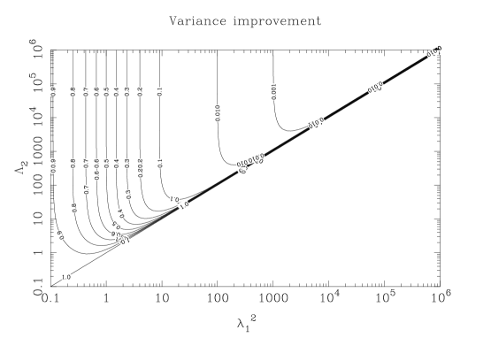
Figure 1: Ratio of optimal variance to the equal weighting variance.

The sums over galaxy pairs may be estimated by integrals over the mean number density of the survey, assuming that we have accurate comoving galaxy distances which could come from a spectroscopic redshift survey such as the Sloan spectroscopic galaxy sample. Redshifts can be converted into distance coordinates $w$ using the approximate formulae in ?.

In order to set the weights, we need to compute

$$\Lambda_{n} = \left({f\over\sigma_{\rm pair}}\right)^{n}\sum_{a,b}\langle I_{ab}\rangle^{n}$$ (24)

$$\simeq 2\pi\theta\Delta\theta\Delta\Omega\left({f\over\sigma_{\rm pair}}\right)^{n}\int dw_{a}dw_{b}$$

$$\eta_{I}^{n}(R_{ab})\phi_{w}(w_{a})\phi_{w}(w_{b})\left[1+\xi(R_{ab})\right]$$

where the selection function $\phi_{w}(w)$ is the number of objects at distance $w$ included in the survey, and $\xi$ is the galaxy two-point correlation function. $\phi_{w}$ is related to the redshift selection function $\phi_{z}$ by $\phi_{w}dw=\phi_{z}dz$ and we use the redshift distribution of the form.

$$\phi_{z}(z)\,\propto\,z^{2}\exp\left[-\left(\frac{z}{z_{0}}\right)^{1.5}\right]$$ (25)

where the median redshift of the survey is $z_{m}\approx 1.4z_{0}$. This is normalised by $\int dz\,\phi_{z}(z)=n_{\rm str}$, where $n_{\rm str}$ is the number of galaxies per steradian in the survey. Note that for $n=0$ we calculate $N$, the expected number of pairs at separation between $\theta$ and $\theta+\Delta\theta$. For $\sigma_{\rm pair}$, we assume that the dispersion in ellipticity is $\sigma_{e}\sim 0.2$, (?), giving $\sigma_{\rm pair}\sim 0.04$.

Typically, for angular scales less than $\theta\simeq 15$ arcminutes, we find that $\lambda_{1}^{2}\ll\Lambda_{2}$. The ratio, equation 23, is then simply $\lambda_{1}^{-2}$, and the optimally-weighted error is almost pure shot-noise $\sigma^{2}_{L}\approx\sigma^{2}_{\rm pair}/N$. Changing $\Delta\theta$ predominantly alters $N$ and hence the amplitude of the shot noise component.

Note that the weights are not constrained to be positive and in extreme cases, if $J_{p}$ is large, can be negative. The reason for this is that the contribution to the error from intrinsic alignments is assumed to be proportional to the intrinsic alignment signal itself. If this is the dominant error term, it is possible that one can have a net gain by reducing this term through giving some pairs negative weight. This behaviour is, however, rare.

4 Results for the Sloan Spectroscopic Sample: Comparison of HRH and Jing intrinsic alignment models

Covering $\pi$ steradian the Sloan Digital Sky Survey, SDSS, is a wide, shallow survey. The spectroscopic galaxy sample has a median redshift of 0.1 with redshift measurements known to an accuracy of $\Delta z=0.0001$ (?). Figure 2 shows the reduced intrinsic alignment error calculated using the optimal weighting scheme, compared to the error introduced to the lensing signal by an unweighted HRH intrinsic alignment signal and an unweighted Jing intrinsic alignment signal at a redshift of 0.1. The minimised signal for both intrinsic alignment models is close to pure shot noise with residuals of less than 1%.

Figure 2: Reduction in the error from intrinsic alignments and shot noise for the Sloan spectroscopic sample. The upper curves show the error in the shear correlation function for two intrinsic alignment models, assuming all galaxy pairs are weighted equally. Note that these curves essentially combine a statistical error (shot noise) with a systematic contamination (intrinsic alignments). Triangles show the Jing model and circles HRH’s spiral model. The error with optimal weighting is shown as filled circles, and has reduced both intrinsic alignment model signals close to shot noise (shown dashed). Note that the increase in shot noise is negligible due to the small proportion of downweighted pairs in the optimal weighting scheme. The expected weak gravitational lensing correlation function for a $\Lambda$CDM model, (dotted), is still dominated by shot noise for this shallow $z_{m}=0.1$ sample.

The published differences between the HRH and Jing models come from from the higher resolution N-body simulation used by Jing, and differences in the choice of $\xi(R)$. Jing finds that the spatial ellipticity correlation of the halos, $\eta_{I}(R)$, derived for the same minimum dark matter halo mass, is higher by a factor of 2, compared to the elliptical HRH model. This model assumes that the ellipticity of the galaxy is the same as that of the parent halo. It is sensitive to the accuracy of the halo shape measurement and is therefore better determined in the higher resolution simulations. A second difference, in the angular intrinsic ellipticity correlation, arises since Jing uses a larger two-point correlation function, measured from the simulation itself, whereas HRH assumed $\xi(R)=(R\,/\,5h^{-1}{\rm Mpc})^{-1.8}$. HRH also used a model for spiral galaxies, where the galaxy is modelled as a thin disk, perpendicular to the angular momentum vector of the parent halo. The spiral model has significantly lower correlations at spatial separations $R_{ab}\mathrel{\raise 1.16pt\hbox{$>$}\kern-7.0pt\lower 3.06pt\hbox{{$\scriptstyle\sim$}}}5h^{-1}{\rm Mpc}$.

Except where otherwise stated, we use the HRH spiral model throughout this paper. $\eta_{I}(R)$, summed over $e_{1}$ and $e_{2}$, is fitted by an exponential: $\eta_{I}(R)=0.012\exp(-R/[1.5h^{-1}Mpc])$. We should point out that fitting an exponential model could underestimate $\eta_{I}(R)$ on large scales $R>10{\rm h}^{-1}{\rm Mpc}$, where the signal-to-noise is low. This would then lead to an underestimation of the intrinsic signal on angular scales $\theta\geq 10^{\prime}$. If this were the case, however, the results would be inconsistent with the lack of detection of a B mode signal on these scales found by ?, discussed further in section 6. Figure 2 shows the contamination expected from this exponential HRH model and the larger signal found by ?, assuming the same minimum halo mass as HRH ($6.9\times 10^{11}{\rm M}_{\odot}$). We have, however, used the power-law two-point correlation function to convert the Jing $\eta_{I}(R)$ fitting formula into an angular signal. Increasing the minimum halo mass increases the unweighted Jing signal, but does not greatly affect the minimised signal leaving residuals at less than 3% of the shot noise.

As the Sloan spectroscopic sample is so shallow, the expected lensing signal is negligible preventing this spectroscopic sample from being used as a weak lensing data set. It is however an interesting test of the method showing that the optimal weighting scheme will almost completely remove both the HRH and the stronger Jing model for intrinsic alignments. We will therefore proceed with the HRH spiral model for intrinsic alignment, as the method has been shown to remove successfully any amplitude of intrinsic alignment provided the signal is significant only for galaxy pairs closer than a few tens of Mpc.

5 Using Photometric Redshifts

The method detailed in section 3 is only feasible for spectroscopic surveys with essentially known galaxy distances. More typically we have good estimates of galaxy distances from photometric redshifts with associated errors. These errors are much larger than the scale over which the intrinsic alignments are correlated. We must therefore define a new weighting scheme for galaxy pairs dependent on their estimated redshifts alone. Those weights are then transformed into an average weight assigned to a pair at true redshift separation to calculate the residual angular intrinsic contribution.

Survey	size str	$z_{m}$	$\Delta_{z}$
Sloan spectroscopic sample	$\pi$	0.1	0.0001
SDSS photometric	$\pi$	0.2	0.025
COMBO-17	0.0005	0.6	0.03
RCS BVRz’	0.015	0.56	0.3
ODT UBVRIz’	0.005	1.0	0.2

Table 1: Survey parameters for SDSS, COMBO-17, RCS and ODT

Using the minimum lensing error derived in section 3 as a benchmark we propose a simpler approach to derive the weightings for galaxies at estimated distances. Applying the accuracy of the Sloan spectroscopic sample, $\Delta_{z}=0.0001$, to this alternative method we come very close to reproducing the previously derived minimum. This shows that our alternative method, in the limit of accurate photometric redshift information, is close to the optimal result. As the errors in the distance measurements increase, our ability to down-weight close galaxy pairs correctly decreases, and the residual intrinsic contamination increases.

For a pair of galaxies with estimated redshift $\hat{z}_{a}$ and $\hat{z}_{b}$ we assign a zero weight if $|\hat{z}_{a}-\hat{z}_{b}|<\alpha\Delta_{z}$ and a weight of one otherwise. We choose $\alpha$ to minimise the total error on the shear correlation function. The optimum value depends on angular separation, and survey details. Clearly, this is not the most general weighting scheme, but we will see later that, with good photometric redshifts, this simple procedure does almost as well as the theoretical optimum where all galaxy distances are known. Assuming that the estimated redshifts are distributed normally about the true redshifts with Gaussian widths given by $\Delta_{z}$, we find that the average weight for a galaxy pair at true redshifts $z_{a}$ and $z_{b}$ is given by

$$\langle W_{ab}\rangle=1-\frac{1}{2\sqrt{\pi}}\int dx\,{\rm e}^{-x^{2}}\left[{\rm erf}(y+x)-{\rm erf}(v+x)\right]$$ (26)

where

$$x\equiv\frac{\hat{z}_{a}-z_{a}}{\sqrt{2}\,\Delta_{z}}\,\,\,\,y\equiv\frac{z_{a}-z_{b}+\alpha\Delta_{z}}{\sqrt{2}\,\Delta_{z}}\,\,\,\,v\equiv\frac{z_{a}-z_{b}-\alpha\Delta_{z}}{\sqrt{2}\,\Delta_{z}}$$ (27)

The weighted intrinsic component can then be evaluated using the integral version of equation 11, setting the value of $\alpha$ by minimising the total error contribution from the intrinsic alignments, $\sigma_{IA}$ and the shot noise, $\sigma_{SN}$.

$$\sigma_{IA}=\frac{f\int dz_{a}dz_{b}\phi_{z}(z_{a})\phi_{z}(z_{b})\left[1+\xi(R_{ab})\right]\langle W_{ab}\rangle\eta_{I}(R_{ab})}{\int dz_{a}dz_{b}\phi_{z}(z_{a})\phi_{z}(z_{b})\left[1+\xi(R_{ab})\right]\langle W_{ab}\rangle}$$ (28)

$$\sigma_{SN}=\sigma_{\rm pair}\left(\int dz_{a}dz_{b}\phi_{z}(z_{a})\phi_{z}(z_{b})\left[1+\xi(R_{ab})\right]\langle W_{ab}\rangle\right)^{-1}$$ (29)

As $\alpha$ increases the probability of removing all close galaxy pairs increases and the intrinsic contribution decreases to zero. This means that the total galaxy count decreases and the shot noise increases, hence there is an optimum value of $\alpha$. As $\theta$ increases, shot noise begins to dominate the intrinsic alignment error, and a progressively lower value of $\alpha$ is favoured. This is shown in figure 3 where the reduced intrinsic contamination is plotted for varying values of $\alpha$ for a low accuracy photometric redshift survey, for example the ODT.

The optimum values of $\alpha$ are dependent on survey size, depth, photometric redshift accuracy and the choice of $\eta_{I}(R)$.

Figure 3: Residual error expected after removing pairs within $\alpha\Delta_{z}$ of each other for the ODT survey. $\Delta_{z}$ is the root mean square photometric redshift error.

6 Application of semi-optimised weighting scheme to multi-colour survey designs

We consider four multi-colour surveys with varying depth, angular size and photometric redshift accuracy: Sloan photometric survey, SDSS, COMBO-17, the RCS survey and the ODT survey. Table 1 details the relevant survey parameters. The uncertainty in the redshift depends mainly on the number of colours known for each object. Photometric redshift errors for SDSS assumes a neural-network-based photometric redshift estimator (?; ?). For the RCS and ODT we assume the use of hyper-z (?). The full COMBO-17 survey has imaging to $R\sim 25.5$, but colour information in 17 bands (producing very accurate photometric redshift estimates) down to a limiting magnitude of $R\sim 24$. It is this magnitude-limited sample of the full COMBO-17 weak lensing survey which we will consider.

Figure 4 shows the correlation signal we expect to find from HRH-derived intrinsic alignments and the best reduction that can be achieved with this method, with photometric redshift information at the accuracy appointed for each survey. These have been calculated using the values of $\alpha(\theta)$ shown in figure 5. The dashed line in Figure 4 shows the optimal improvement in the error obtainable if accurate distances were known, using the method detailed in section 3. This acts as a useful benchmark to see how close the semi-optimal method for multi-colour surveys gets to the ideal. The intrinsic alignment signals can be compared to the expected weighted lensing signal, equation 42, for each survey. This is derived from a nonlinear CDM mass power spectrum with $\Omega_{m}=0.3$, $\Omega_{\Lambda}=0.7$, $\Gamma=0.21$, $\sigma_{8}=0.9$, calculated using the ‘halo model’ fitting formula (?). For the pair weighting proposed, this signal is slightly lower than the unweighted lensing signal (equation 2), (see Appendix).

Figure 4: Reduction in the error from intrinsic alignments and shot noise for photometric SDSS, RCS, COMBO-17 and ODT. The semi-optimal weighting, (filled circles), has reduced the unweighted HRH intrinsic alignment error (circles) to well below the expected amplitude of the weighted weak lensing shear signal, (dotted). The effect of semi-optimal weighting can be compared to the optimally weighted error, (dashed), attainable with spectroscopic redshifts.

Figure 5: Optimum values of $\alpha$ for the four different surveys, assuming the HRH spiral model for intrinsic alignments. The dashed line shows the optimal values of $\alpha$ for the ODT survey, assuming the higher intrinsic signal found by Jing (2002). At the expense of marginally-higher residual shot noise, this conservative pruning of the pairs virtually guarantees almost complete removal of the intrinsic alignment contamination.

The true amplitude of the intrinsic alignment signal is rather uncertain; the correlation signal from intrinsic alignments could move up, as argued by ?, or down, as argued, for example, by ?, and by up to an order of magnitude. Figure 5 also shows the optimum $\alpha(\theta)$ if the intrinsic alignment signal is as high as found by ?, for the ODT survey. Due to the presence of intrinsic correlations at larger galaxy pair spatial separations, it is necessary to remove more pairs at larger angular scales. At the expense of a higher residual shot noise, this more-or-less guarantees removal of any plausible intrinsic alignment signal, leaving errors at less than 3% of the weighted ODT lensing signal. This is probably the preferred strategy until the intrinsic signal is better determined, but it should be noted that an intrinsic alignment signal of the amplitude found by ? is incompatible with current weak lensing detections, (?).

Using an HRH model for intrinsic alignments we find that the SDSS is dominated by intrinsic alignments and that the weak lensing signal from the two middle-depth surveys, RCS and COMBO-17, will be strongly contaminated at angular scales less than 10 arcminutes. Interestingly ? show an E/B mode decomposition for the RCS survey which shows a significant B mode at angular scales less than 10 arcminutes. The presence of a B mode can be due, on small angular scales, to source clustering, (?), or it can imply systematics within the data and/or the presence of intrinsic galaxy alignments (?).

The application of the weighting scheme produces encouraging results, the most startling of which comes from the SDSS. Due to the wide sky coverage and accurate photometric redshift information it is possible to reduce the intrinsic alignment signal from well above, to well below the expected lensing signal. This enables, in principle, the extraction of a lensing signal at angular scales, $\theta>1^{\prime}$, with errors less than $10\%$. We see similar reductions for the other three surveys, with the success of the reduction dependent on the accuracy of the redshift estimates.

7 Conclusions and implications for future weak lensing surveys

In this paper we have shown how distance information can be used to reduce the contamination of the weak gravitational lensing shear signal by the intrinsic alignments of galaxies. Our principal finding is that the level of intrinsic ellipticity correlation in the shear correlation function can be reduced by up to several orders of magnitude, by down-weighting appropriately the contribution from pairs of galaxies which are likely to be close in three dimensions.

For spectroscopic surveys we have derived an optimal galaxy pair weighting which reduces the contamination to a negligible component, leaving almost pure shot noise. Application of the technique to the relatively shallow Sloan spectroscopic galaxy sample reduces the error by up to two orders of magnitude, but still leaves the lensing signal undetectable, dominated now by shot noise.

For multi-colour surveys with photometric redshift estimates we have proposed a partially-optimised method, which removes pairs with close photometric redshifts from the computation of the shear correlation function. We find that with accurate photometric redshifts this simple method is almost as effective as the fully optimised method. We show that, even with relatively crude photometric redshift estimates, the contamination by intrinsic alignments can be significantly reduced.

Similar conclusions were independently drawn by ? who simultaneously proposed a weighting scheme based on photometric redshifts. Our technique however requires the assumed knowledge of a model for the intrinsic alignments. Provided one is conservative, assuming the largest feasible model, this weighting scheme will reduce the true intrinsic alignment contamination to lensing correlation signals to a negligible level.

We have applied the method to four multi-colour survey designs. The shallow photometric SDSS survey with $z_{m}\sim 0.2$, shows the most dramatic of improvements. The intrinsic alignment signal is expected to dominate completely the weak lensing shear signal from a survey of this depth, but with judicious removal of pairs within $\sim 0.14$ in estimated redshift, the error from shot noise and intrinsic alignments is reduced to only $\sim 10\%$ of the expected shear signal. This opens up the possibility of using the SDSS for future cosmic shear studies. With deeper surveys, such as the RCS, COMBO-17 and the ODT survey, intrinsic alignments in the weak lensing shear signal are significantly reduced. With the highly accurate photometric redshifts of COMBO-17, the reduction is close to optimal, reducing the largely systematic $\sim 220\%$ error at small angular scales to a much smaller and largely statistical error of $\sim 17\%$ of the expected lensing shear correlation. This limiting error is predominantly shot noise which will decrease as the survey size grows. The ODT and RCS have less accurate distance estimates but even with current photometric redshift estimates, which undoubtedly will improve with time, the reduction is quite significant. For the wide RCS, the 130% contamination at angular scales $\theta\sim 2^{\prime}$, is reduced to an error $\sim 20\%$. For deep multi-colour surveys such as the ODT, the intrinsic alignment signal is almost completely removed, leaving noise at a level of $\leq 2$% of the lensing signal.

The aim for weak lensing surveys to date has been to go as deep and as wide as possible. With an increase in depth comes an increase in the expected lensing signal and for purely geometrical reasons we also see a decrease in intrinsic alignment correlations. To reduce shot noise, the error introduced by the intrinsic ellipticity distribution of galaxies, surveys can go wide and/or deep. This increases the number of lensed sources, in the limit of an infinite number of galaxies the shot noise goes to zero. One additional source of error so far unmentioned is cosmic variance which, for small area surveys, can dominate on scales larger than a few arcminutes, (?). This can be reduced by sampling different areas of the sky and combining to produce a wide field survey. Note that downweighting close galaxy pairs affects this random error little, whilst effectively removing the systematic errors from intrinsic contamination.

As the size of future lensing surveys increase, control of systematic errors becomes increasingly important. Intrinsic alignment contamination is a potentially large source of error, even if it is at a level much lower than assumed here. This paper has shown that with the addition of accurate photometric redshift information, the presence of intrinsic alignments can be effectively removed. ? have shown that it is possible to extract a low weak lensing signal from a survey with a median redshift of 0.56 and argue that using this shallower survey enables more accurate star-galaxy separation and provides a fairly well determined redshift distribution for the sources, another uncertainty in weak lensing measurements to date. The addition of depth information to weak lensing studies also opens new possibilities for the application of lensing tomography (?; ?), and reconstruction of the full 3D cosmological mass distribution (?; ?), but here we have concentrated only on its benefits in reducing intrinsic alignment contamination. In view of the dramatic improvements it offers lensing signal detection we therefore propose that for future weak lensing surveys, emphasis should be placed on acquiring multi-colour data in a wide area. In the case of restricted telescope time, moderate depth surveys, $z_{m}\sim 0.6$, may then become a more attractive alternative to ultra-deep observations, $z_{m}>1.0$, that can often be limited by seeing.

8 Acknowledgements

We are very grateful to Rob Smith for providing us with his nonlinear power spectrum fitting formula and code. We thank Yipeng Jing, Michael Brown and Emily MacDonald for useful discussions and the referee for helpful comments.

Appendix A Theoretical lensing signal for weighted ellipticities

The effective convergence is (?, equation 6.18)

$$\bar{\kappa}_{\rm eff}(\overrightarrow{\theta})=A\int_{0}^{\infty}dwg(w)f_{K}(w){\delta[f_{K}(w)\overrightarrow{\theta},w]\over a(w)}$$ (30)

where $A=3H_{0}^{2}\Omega_{m}/(2c^{2})$, $g(w)$ is the weighting function given in equation 4, and $f_{K}(w)$ is the geometry-dependent comoving angular diameter distance, dependent on the curvature $K$,

$$f_{K}(w)=\left\{\begin{array}[]{ll}K^{-1/2}\sin(K^{1/2}w)&(K>0)\\ w&(K=0)\\ (-K)^{-1/2}\sinh[(-K)^{1/2}w]&(K<0)\\ \end{array}\right.\;.$$ (31)

Note that $w$, the comoving radial geodesic distance, plays two roles, both as a third spatial coordinate, and as a time evolution label.

The effective 2D convergence is an integral of the 3D convergence, and it is this which we will weight, since each galaxy gives an estimate of the shear, or convergence, in the weak lensing limit.

$$\bar{\kappa}_{\rm eff}(\overrightarrow{\theta})=\int_{0}^{\infty}dw\,\phi(w)\kappa_{\rm eff}(\overrightarrow{\theta},w).$$ (32)

We will weight 3D convergence estimates with a weight function $H(w,w^{\prime},|\overrightarrow{\theta}|)$, to give the weighted correlation function

$$\langle\bar{\kappa}_{\rm eff}(\overrightarrow{\theta})\bar{\kappa}_{\rm eff}^{*}(\overrightarrow{\theta}^{\prime})\rangle = {1\over Q}\int_{0}^{\infty}dw\int_{0}^{\infty}dw^{\prime}\,H(w,w^{\prime},|\overrightarrow{\theta}-\overrightarrow{\theta}^{\prime}|)\langle\kappa_{\rm eff}(\overrightarrow{\theta},w)\kappa^{*}_{\rm eff}(\overrightarrow{\theta}^{\prime},w^{\prime})\rangle\phi(w)\phi(w^{\prime})$$ (33)

$$= B\int_{0}^{\infty}dw\int_{0}^{\infty}dw^{\prime}\,\phi(w)\phi(w^{\prime})H(w,w^{\prime},|\overrightarrow{\theta}-\overrightarrow{\theta}^{\prime}|)\int_{0}^{w}dw_{1}{f_{K}(w_{1})f_{K}(w-w_{1})\over f_{K}(w)a(w_{1})}$$

$$\int_{0}^{w^{\prime}}dw_{2}{f_{K}(w_{2})f_{K}(w^{\prime}-w_{2})\over f_{K}(w^{\prime})a(w_{2})}\langle\delta(f_{K}(w_{1})\overrightarrow{\theta},w_{1})\delta^{*}(f_{K}(w_{2})\overrightarrow{\theta}^{\prime},w_{2})\rangle$$

where $Q\equiv\int_{0}^{\infty}\int_{0}^{\infty}dwdw^{\prime}\,H(w,w^{\prime},\theta)\phi(w)\phi(w^{\prime})$ and $B\equiv A^{2}/Q$. We now assume that the scale over which the correlations of density are non-zero is small, in the sense that there is negligible evolution of the density field over the light-crossing time of the correlation scale. Writing

$$\delta({{\bf x}})=\int{d^{3}{\bf k}\over(2\pi)^{3}}\delta_{\bf k}(w)\exp(-i{\bf k}\cdot{\bf x})$$ (34)

and using homogeneity of $\delta$ to define the power spectrum of the density field $P$,

$$\langle\delta_{\bf k}(w)\delta^{*}_{{\bf k}^{\prime}}(w^{\prime})\rangle=(2\pi)^{3}P(k,w)\delta^{D}({\bf k}-{\bf k}^{\prime})$$ (35)

where $\delta^{D}$ is a Dirac delta function. Hence

$$\langle\bar{\kappa}_{\rm eff}(\overrightarrow{\theta})\bar{\kappa}_{\rm eff}^{*}(\overrightarrow{\theta}^{\prime})\rangle = B\int_{0}^{\infty}dw\int_{0}^{\infty}dw^{\prime}\,\phi(w)\phi(w^{\prime})H(w,w^{\prime},|\overrightarrow{\theta}-\overrightarrow{\theta}^{\prime}|)\int_{0}^{w}dw_{1}\int_{0}^{w^{\prime}}dw_{2}F(w,w_{1})F(w^{\prime},w_{2})$$ (36)

$$\int{d^{3}{\bf k}\over(2\pi)^{3}}\exp[-i{\bf k}_{\perp}\cdot(f_{K}(w_{1})\overrightarrow{\theta}-f_{K}(w_{2})\overrightarrow{\theta}^{\prime})]\exp[ik_{z}(w_{1}-w_{2})]P(k,w_{1})$$

where ${\bf k}=({\bf k}_{\perp},k_{z})$ and

$$F(w,w^{\prime})\equiv{f_{K}(w^{\prime})f_{K}(w-w^{\prime})\over f_{K}(w)a(w^{\prime})}$$ (37)

Now we make the standard approximation that the correlation function of $\delta$ is non-zero only if $w_{1}$ and $w_{2}$ are almost equal. Specifically, we assume that $F$ and $f_{K}$ don’t vary much over this scale. Thus we set $f_{K}(w_{1})=f_{K}(w_{2})$ in the first exponential, and also approximate $F(w^{\prime},w_{2})\simeq F(w^{\prime},w_{1})$. The $w_{2}$ integral then simplifies, since it is approximately

$$\int_{0}^{\infty}dw_{2}\exp(-ik_{z}w_{2})=2\pi\delta^{D}(k_{z})$$ (38)

and we are left with

$$\langle\bar{\kappa}_{\rm eff}(\overrightarrow{\theta})\bar{\kappa}_{\rm eff}^{*}(\overrightarrow{\theta}^{\prime})\rangle = B\int_{0}^{\infty}dw\int_{0}^{\infty}dw^{\prime}\,\phi(w)\phi(w^{\prime})H(w,w^{\prime},|\overrightarrow{\theta}-\overrightarrow{\theta}^{\prime}|)\int_{0}^{w}dw_{1}F(w,w_{1})F(w^{\prime},w_{1})$$ (39)

$$\int{d^{3}{\bf k}_{\perp}\over(2\pi)^{2}}\exp[-i{\bf k}_{\perp}\cdot f_{K}(w_{1})(\overrightarrow{\theta}-\overrightarrow{\theta}^{\prime}))]\exp[ik_{z}w_{1}]P(|{\bf k}_{\perp}|,w_{1}).$$

An angle integration of $P$ gives

$$\int{d^{3}{\bf k}_{\perp}\over(2\pi)^{2}}\exp[-i{\bf k}_{\perp}\cdot f_{K}(w_{1})(\overrightarrow{\theta}-\overrightarrow{\theta}^{\prime}))]P(|{\bf k}_{\perp}|)=\int_{0}^{\infty}{kdk\over 2\pi}P(k,w_{1})J_{0}[kf_{K}(w_{1})|\overrightarrow{\theta}-\overrightarrow{\theta}^{\prime}|]$$ (40)

where $J_{0}$ is the zeroth Bessel function of the first order. Hence we can write the correlation function as

$$\langle\bar{\kappa}_{\rm eff}(\overrightarrow{\theta})\bar{\kappa}_{\rm eff}^{*}(\overrightarrow{\theta}^{\prime})\rangle = B\int_{0}^{\infty}dw\int_{0}^{\infty}dw^{\prime}\,\phi(w)\phi(w^{\prime})H(w,w^{\prime},|\overrightarrow{\theta}-\overrightarrow{\theta}^{\prime}|)\int_{0}^{w}dw_{1}F(w,w_{1})F(w^{\prime},w_{1})$$ (41)

$$\int_{0}^{\infty}{kdk\over 2\pi}P(k,w_{1})J_{0}[kf_{K}(w_{1})|\overrightarrow{\theta}-\overrightarrow{\theta}^{\prime}|].$$

Writing this in a form as close to equation 2 as possible, by reversing the order of integration, and noting that in the weak lensing limit, shear and convergence have the same statistical properties; $\langle\gamma(\overrightarrow{\theta})\gamma^{*}(\overrightarrow{\theta}^{\prime})\rangle=\langle\bar{\kappa}_{\rm eff}(\overrightarrow{\theta})\bar{\kappa}_{\rm eff}^{*}(\overrightarrow{\theta}^{\prime})\rangle$, we find:

$$\langle\gamma(\overrightarrow{\theta})\gamma^{*}(\overrightarrow{\theta}^{\prime})\rangle=B\int_{0}^{\infty}dw_{1}X(w_{1},|\overrightarrow{\theta}-\overrightarrow{\theta}^{\prime}|)\int_{0}^{\infty}{kdk\over 2\pi}P(k,w_{1})J_{0}[kf_{K}(w_{1})|\overrightarrow{\theta}-\overrightarrow{\theta}^{\prime}|].$$ (42)

where

$$X(w_{1},\theta)\equiv\int_{w_{1}}^{\infty}dw\int_{w_{1}}^{\infty}dw^{\prime}\phi(w)\phi(w^{\prime})F(w,w_{1})F(w^{\prime},w_{1})H(w,w^{\prime},\theta).$$ (43)

In the equal-weighted case, $H=1$, and $X(w,\phi)$ simplifies to the product of two equal integrals, each independent of $\phi$ and equal to $g(w)f_{K}(w)/a(w)$.

The effect of the weighting is shown in Fig. 6. For surveys such as COMBO-17 with accurate photometric redshifts, the lensing signal changes by up to $\sim 3\%$. For the Sloan photometric survey, the effect is $\sim 10\%$; the greatest effect is for RCS, which has the least accurate photometric redshifts.

Figure 6: Expected weak lensing signal for a $\Lambda CDM$ model with $\sigma_{8}=0.9$, for the surveys discussed in the main text. The solid line shows equal weighting of galaxies; the dotted line shows the effect of employing the proposed multi-colour survey weighting scheme.

References

- [Allen, Dalton & Moustakas¡2002¿] Allen P., Dalton G., Moustakas L., 2002. in preperation, .
- [Bacon et al.¡2002¿] Bacon D., Massey R., Refregier A., Ellis R., 2002. MNRAS, submitted, astroph/0203134, .
- [Bartelmann & Schneider¡2001¿] Bartelmann M., Schneider P., 2001. Physics Reports, 340, 291.
- [Bolzonella, Miralles & Pello¡2000¿] Bolzonella M., Miralles J., Pello R., 2000. A& A, 363, 476.
- [Brown et al.¡2002a¿] Brown M., Taylor A., Bacon D., Gray M., Dye S., Meisenheimer K., Wolf C., 2002a. MNRAS, submitted, astroph/0210213, .
- [Brown et al.¡2002b¿] Brown M., Taylor A., Hambly N., Dye S., 2002b. MNRAS, 333, 501.
- [Catelan, Kamionkowski & Blandford¡2001¿] Catelan P., Kamionkowski M., Blandford R. D., 2001. MNRAS, 320, L7.
- [Crittenden et al.¡2001¿] Crittenden R., Natarajan R., Pen U., Theuns T., 2001. ApJ, 559, 552.
- [Crittenden et al.¡2002¿] Crittenden R., Natarajan R., Pen U., Theuns T., 2002. ApJ, 568, 20.
- [Croft & Metzler¡2000¿] Croft R. A. C., Metzler C. A., 2000. ApJ, 545, 561.
- [Firth, Lahav & Somerville¡2002¿] Firth A., Lahav O., Somerville R., 2002. MNRAS, submitted, astroph/0203250, .
- [Heavens, Refregier & Heymans¡2000¿] Heavens A., Refregier A., Heymans C., 2000. MNRAS, 319, 649.
- [Hoekstra et al.¡2002a¿] Hoekstra H., Van Waerbeke L., Gladders M., Mellier Y., Yee H., 2002a. ApJ, 577, 604.
- [Hoekstra et al.¡2002b¿] Hoekstra H., Yee H., Gladders M., Barrientos L. F., Hall P., Infante L., 2002b. ApJ, 572, 55.
- [Hoekstra, Yee & Gladders¡2001¿] Hoekstra H., Yee H., Gladders M., 2001. ApJ, 558, L11.
- [Hoekstra, Yee & Gladders¡2002¿] Hoekstra H., Yee H., Gladders M., 2002. ApJ, 577, 595.
- [Hu & Keeton¡2002¿] Hu W., Keeton C., 2002. Phys. Rev. D., submitted, astroph/0205412, .
- [Hu¡1999¿] Hu W., 1999. ApJ, 552, L21.
- [Hu¡2002¿] Hu W., 2002. Phys. Rev. D., submitted, astroph/0208093, .
- [Hudson et al.¡1998¿] Hudson M., Gwyn S., Dahle H., Kaiser N., 1998. ApJ, 501, 531.
- [Hui & Zhang¡2002¿] Hui L., Zhang J., 2002. ApJ, submitted, astroph/0205512, .
- [Jing¡2002¿] Jing Y. P., 2002. MNRAS, 335, L89.
- [King & Schneider¡2002¿] King L., Schneider P., 2002. A&A, submitted, astroph/0208256, .
- [Lee & Pen¡2001¿] Lee J., Pen U., 2001. ApJ, 555, 106.
- [Pen¡1999¿] Pen U., 1999. ApJ Suppl., 120, 49.
- [Porciani, Dekel & Hoffman¡2002¿] Porciani C., Dekel A., Hoffman Y., 2002. MNRAS, 332, 325.
- [Rhodes, Refregier & Groth¡2001¿] Rhodes J., Refregier A., Groth E., 2001. ApJ(Lett), 552, 85.
- [R.Maoli et al.¡2001¿] R.Maoli, Van Waerbeke L., Mellier Y., Schneider P., Jain B., Bernardeau F., Erben T., 2001. A& A, 368, 766.
- [Schneider et al.¡2002¿] Schneider P., van Waerbeke L., Kilbinger M., Mellier Y., 2002. A&A, submitted, astroph/0206182, .
- [Schneider, Van Waerbeke & Mellier¡2002¿] Schneider P., Van Waerbeke L., Mellier Y., 2002. A& A, 389, 741.
- [Smith et al.¡2002¿] Smith R., Peacock J., Jenkins A., White S., Frenk C., Pearce F., Thomas P., Efstathiou G., Couchman. H., 2002. MNRAS, submitted, astroph/0207664, .
- [Stoughton & SSDS Team¡2002¿] Stoughton C., SSDS Team, 2002. AJ, 123, 485.
- [Tagliaferri et al.¡2002¿] Tagliaferri R., Longo G., Andreon S., Capozziello S., Donalek C., Giordano G., 2002. astroph/0203445, .
- [Taylor¡2001¿] Taylor A., 2001. Phys. Rev. Lett, submitted, astroph/0111605, .
- [Van Waerbeke et al.¡2001¿] Van Waerbeke L., Mellier Y., Radovich M., Bertin E., Dantel-Fort M., McCracken H., Fevre O. L., Foucaud S., Cuillandre J., Erben T., Jain B., Schneider P., Bernardeau F., Fort B., 2001. A& A, 374, 757.
- [Van Waerbeke, Mellier & Tereno¡2002¿] Van Waerbeke L., Mellier Y., Tereno I., 2002. astroph/0206245, .
- [Wolf, Meisenheimer & Röser¡2001¿] Wolf C., Meisenheimer K., Röser H., 2001. A& A, 365, 660.