Exploring the Expansion History of the Universe

Abstract

Exploring the recent expansion history of the universe promises insights into the cosmological model, the nature of dark energy, and potentially clues to high energy physics theories and gravitation. We examine the extent to which precision distance-redshift observations can map out the history, including the acceleration-deceleration transition, and the components and equations of state of the energy density. We consider the ability to distinguish between various dynamical scalar field models for the dark energy, as well as higher dimension and alternate gravity theories. Finally, we present a new, advantageous parametrization for the study of dark energy.

I Introduction

The quest to explore the expansion history of the universe has carried cosmology well beyond “determining two numbers” – the present dimensionless density of matter $\Omega_{m}$ and the present deceleration parameter $q_{0}$ san61 . Observations have advanced so that now cosmologists seek to reconstruct the entire function $a(t)$ representing the expansion history of the universe.

A myriad of cosmological observational tests can probe the function $a(t)$ more fully, over much of the age of the universe (see Sandage san88 , Linder lin89 ; lin97 , Tegmark teg ). This paper concentrates on the most advanced method, the magnitude-redshift relation of Type Ia supernovae.

Just as understanding the thermal history of the early universe has taught us an enormous amount about both cosmology and particle physics (see, e.g., kt ), the recent expansion history of the universe promises similarly fertile ground with the discovery of the current acceleration of the expansion of the universe. This involves concepts of the late time role of high energy field theories in the form of possible quintessence, scalar-tensor gravitation, higher dimension theories, brane worlds, etc. as well as the fate of the universe.

II Mapping the Expansion History

Type Ia supernovae, or any standardizable candles (sources with known luminosity), are excellently suited to map the expansion history $a(t)$ since there exists a direct relation between the observed distance-redshift relation $d(z)=(1+z)\eta(z)$ and the theoretical $a(t)$. For a flat universe, assumed throughout,

$$\eta(z)=\int_{a_{e}}^{1}da/(a^{2}H)=\int_{0}^{z}dz^{\prime}/H(z^{\prime})\,,$$ (1)

where $\eta$ is the conformal time, $d\eta=dt/a$, the Hubble parameter is $H=\dot{a}/a$ and $a_{e}=1/(1+z)$ is the scale factor at the time of emission, i.e. when the supernova exploded.

The Hubble parameter in general relativity comes from the Friedmann equation

$$H^{2}=(8\pi/3)\rho\,,$$ (2)

and the conservation condition of each component is

$$\dot{\rho}/\rho=-3H(1+p/\rho)\equiv-3H[1+w(z)],$$ (3)

where the energy density is $\rho$, the pressure $p$, and the equation of state (EOS) of each component is defined by $w=p/\rho$. Ordinary nonrelativistic matter has $w=0$; a cosmological constant has $w=-1$. We explicitly allow the possibility that $w$ evolves.

The expansion history $a(t)$ is given by

$$t(a)=\int_{a}^{1}da^{\prime}/(a^{\prime}H)=\int_{0}^{z}dz^{\prime}/[(1+z^{\prime})H(z^{\prime})].$$ (4)

The fly in the ointment is that the measured distance $d(z)$ is related to, but is not, the desired history relation $a(t)$. To translate $d(z)$ into $a(t)$ directly involves a derivative of $d(z)$, so noisy data can introduce difficulties astier ; ht . Instead one finds $H(z)$ through the cosmology parameters $\rho$ and $w(z)$.

Observational evidence for accelerated expansion informs us that there must be a component with a strongly negative EOS – “dark energy” – in addition to matter. Then combining equations (1)-(3):

$$H_{0}\eta(z) = \int_{0}^{z}dz^{\prime}\,\Big{[}\Omega_{m}(1+z^{\prime})^{3}$$

$$\mbox{}+(1-\Omega_{m})e^{-3\int_{0}^{\ln(1+z^{\prime})}d\ln(1+z^{\prime\prime})[1+w(z^{\prime\prime})]}\Big{]}^{-1/2},$$

where $\Omega_{m}$ is the dimensionless matter density $8\pi\rho_{m}/(3H_{0}^{2})$ and $H_{0}=H(0)$ is the Hubble constant. Eq. (4) can then be used to obtain $a(t)$.

To find $w(z)$ one could solve the scalar field equation for a particular theory but this does not allow a model independent parameter space in which to compare models. Instead, for generality of treatment, various parametrizations of $w(z)$ are used.

II.1 Linear $w(z)$

The conventional first order expansion to the EOS, including the critical property of time variation in the EOS, is $w(z)=w_{0}+w_{1}z$. In this case the exponential in (II) resolves to $(1+z)^{3(1+w_{0}-w_{1})}e^{3w_{1}z}$. However this grows increasingly unsuitable at redshifts $z>1$. Analyzing CMB constraints on the distance to the last scattering surface at $z_{lss}=1100$ would be problematic.

II.2 A new parametrization of the equation of state

To extend parametrization of dark energy to redshifts $z>1$, I suggest a new model:

$$w(a) = w_{0}+w_{a}(1-a)$$ (6)

$$= w_{0}+w_{a}z/(1+z).$$ (7)

Here the exponential in (II) resolves to $a^{-3(1+w_{0}+w_{a})}e^{-3w_{a}(1-a)}$.

This new parametrization has several advantages: 1) a manageable 2-dimensional phase space, 2) reduction to the old linear redshift behavior at low redshift, 3) well behaved, bounded behavior for high redshift, 4) high accuracy in reconstructing many scalar field equations of state and the resulting distance-redshift relations, 5) good sensitivity to observational data, 6) simple physical interpretation.

Beyond the bounded behavior, the new parametrization is also more accurate than the old one. For example, in comparison to the exact solution for the supergravity inspired SUGRA model braxm it is accurate in matching $w(z)$ to -2%, 3% at $z=0.5$, 1.7 vs. 6%, -27% for the linear $z$ approximation (the constants $w_{1}$, $w_{a}$ are here chosen to fit at $z=1$). Most remarkably, it reconstructs the distance-redshift behavior of the SUGRA model to 0.2% over the entire range out to the last scattering surface ($z\approx 1100$).

Note that $dw/d\ln(1+z)|_{z=1}=w_{a}/2$; one might consider this quantity a natural measure of time variation (it is directly related to the scalar field potential slow roll factor $V^{\prime}/V$) and $z=1$ a region where the scalar field is most likely to be evolving as the epoch of matter domination changes over to dark energy domination.

The future Supernova/Acceleration Probe (SNAP: snap ) will be able to determine $w_{a}$ to better than $\pm 0.55$ (one expects roughly $w_{a}\approx 2w_{1}$), with use of a prior on $\Omega_{m}$ of 0.03, or to better than 0.3 on incorporating data from the Planck CMB experiment planck . For the advantages of combining supernova and CMB data see fhlt . The CMB information can be folded in naturally in this parametrization, without imposing artificial cutoffs or locally approximating the likelihood surface as required in the $w_{1}$ parametrization. In fact, the new parametrization is even more promising since the sensitivity of the SNAP determinations increases for $w_{0}$ more positive than $-1$ or for positive $w_{a}$ (see, e.g., astier ): the values quoted above were for a fiducial cosmological constant model. For example, SUGRA predicts $w_{a}=0.58$ and SNAP would put error bars of $\sigma(w_{a})\approx 0.25$ on that; this would demonstrate time variation of the EOS at the 95% confidence level. Incorporation of a Planck prior can improve this to the $\approx$99% confidence level: $\sigma(dw/d\ln(1+z)|_{z=1})\approx 0.1$.

II.3 Expansion and density histories

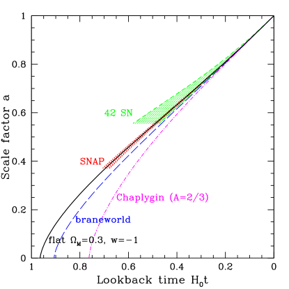
Figure 1 shows the mapping of the expansion history of various models and the constraints that SNAP data would impose. The models include both dark energy and alternative explanations for the acceleration discussed in Sec. III. Regarding the data constraints, it is important to note the presence of correlation between the parameters $\Omega_{m}$, $w_{0}$, and $w_{1}$ or $w_{a}$ (see, e.g., welal ). Despite SNAP being able to determine each individually to high precision, e.g. $\Omega_{m}$ to 0.03, $w_{0}$ to 0.05, $w_{1}$ to 0.3 (each marginalized over others), the correlations among them relax the tightness of the constraint SNAP would place on the expansion history. This is unavoidable (but see Sec. II.4).

Figure 1: Mapping the expansion history through the supernova magnitude-redshift relation can distinguish the dark energy explanation for the accelerating universe from alternate theories of gravitation, high energy physics, or higher dimensions. All three models take an $\Omega_{M}=0.3$, flat universe but differ on the form of the Friedmann expansion equation.

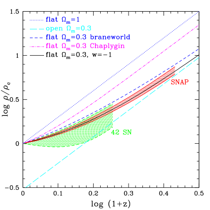
Figure 2 gives the equivalent density history. Note that the matter dominated epoch is characterized by $\rho(z)\sim(1+z)^{3}$ and so has a slope of 3 in this plane. The deviation from this due to the recent epoch of dark energy domination can clearly be seen (cf. Tegmark teg ).

Figure 2: Mapping the density history with SNAP can clearly show both the current accelerating phase and the transition to the matter dominated, decelerating epoch. At high redshifts all models obey the matter dominated slope 3 law, but deviation from this – the sign of dark energy or alternative gravity – is clearly visible for $z<2$.

II.4 Conformal time history

One method of incorporating the advantages of both mapping approaches – the generality of parametrization and the directness of reconstruction – is to consider the conformal time $a(\eta)$. From $d=(1+z)\eta$ one sees that one requires no foreknowledge or local approximation to obtain the scale factor-conformal time relation. The error estimation from the observed magnitudes $m$ is simply

$${\sigma_{\eta}\over\eta}=\sigma_{m}{\ln 10\over 5}\approx(1/2)\sigma_{m}.$$ (8)

A 1% distance measurement error ($\sigma_{m}=0.02$) given by SNAP’s limiting systematics becomes a 1% error in $a(\eta)$.

Another virtue of the conformal time history is its physical interpretation. Consider the logarithmic derivative of the $\eta(a)$ curve. This is

$${d\eta\over d\ln a}=a{dt\over a\,da}=(\dot{a})^{-1}.$$ (9)

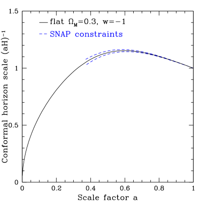
Two simple physical interpretations apply: 1) this gives the proper time evolution of the scale factor, 2) this represents the conformal horizon scale $(aH)^{-1}$. Both are familiar from analysis of inflationary cosmology – they determine when the expansion of the universe enters an accelerating phase.

Figure 3: The conformal horizon scale characterizes the dynamics. The negative slope part of the curve allows comoving wavelengths to expand outside the horizon, or alternately represents $aH=\dot{a}$ increasing, i.e. $\ddot{a}>0$ – the signature of inflation or acceleration. The dashed blue lines show that SNAP will map the accelerating phase, the transition, and into the matter dominated, decelerating phase of the past universe.

Figure 3 maps the conformal horizon. When this curve has positive slope, the expansion is decelerating, $\ddot{a}<0$ and comoving wavelengths (e.g. of density perturbations) enter the horizon. More recently the curve has negative slope; this is the signature of accelerating expansion. In terms of inflation we would say that wavelengths exit the horizon then (the horizon appears to shrink). The dashed lines show the reconstruction possible by SNAP observing supernovae out to $z=1.7$. SNAP clearly has the ability to probe not only the current accelerating epoch (“late time inflation”) but to reach back into the decelerating phase and to map the transition between them.

III Beyond Dark Energy

Mapping the physical time evolution of the scale factor relies on translating the observations into the Hubble parameter $H(z)$. The Friedmann equation (2) related this to the matter and dark energy densities. But ideally we would like to use the data to test the Friedmann equations of general relativity or alternate explanations for the acceleration besides dark energy. Here we lay the framework for such options and give some examples.

III.1 Higher dimension theories

In the braneworld scenario of Deffayet et al. deff , gravitation leaks from the 4-dimensional brane we experience out into the 5-dimensional bulk. The new expansion evolution equation is

$$H^{2}(z)=-ka^{-2}+\left[\sqrt{(8\pi/3)\rho+1/(2r_{c})^{2}}+1/(2r_{c})\right]^{2},$$ (10)

where $r_{c}=M_{Pl}^{2}/(2M_{5}^{3})$ is the crossover scale on which gravity leaks into the bulk, defined in terms of the usual Planck scale $M_{Pl}$ and the 5-dimensional Planck scale $M_{5}$. It is convenient to introduce a dimensionless energy density $\Omega_{rc}=1/(4H_{0}^{2}r_{c}^{2})$. Flatness imposes $\Omega_{rc}=(1-\Omega_{m})^{2}/4$.

SNAP data will be able to constrain the parameter uncertainties to $\sigma(\Omega_{m})=0.008$, or $\sigma(\Omega_{rc})=0.003$ for a fiducial $\Omega_{m}=0.3$. This corresponds to a determination of the crossover scale of $r_{c}=1.43\pm 0.015\,H_{0}^{-1}$. If other observations, analyzed within this braneworld picture, disagreed with this narrow range then this theory could be ruled out. Fig. 1 illustrates how the expansion history for a braneworld model differs from that for dark energy.

Note that other higher dimension models discussed, such as the Randall-Sundrum type 2 model rs2 ; bine and so-called Cardassian expansion freese , reduce to the already discussed dark energy prescription for the recent expansion history.

III.2 Chaplygin gas

A very different possibility to explain the acceleration of the universe is the Chaplygin gas fabris , proposed to unify dark energy and dark matter. Its pressure $p\sim-1/\rho$ gives a solution that at early times behaves like nonrelativistic matter and at late times like a cosmological constant. The expansion equation becomes

$$[H(z)/H_{0}]^{2}=\Omega_{m}(1+z)^{3}+(1-\Omega_{m})\sqrt{A+(1-A)(1+z)^{6}}.$$ (11)

The factor $A$ is interpreted as the sound velocity squared of the Chaplygin gas. As $A\to 1$, it reduces to the cosmological constant.

SNAP data will be able to constrain the parameter uncertainties to $\sigma(\Omega_{M})$$=+0.005,-0.017$ and $\sigma(A)=-0.005$ for a fiducial $\Omega_{m}=0.3$, $A=1$ (though the results are fairly insensitive to $A$). Note dark matter in the form of “quintessence clumps” would require $A$ significantly smaller than unity.

IV Conclusion

The geometry, dynamics, and composition of the universe are intertwined through the theory of gravitation governing the expansion of the universe. By precision mapping of the recent expansion history we can hope to learn about all of these. The brightest hope for this in the near future is the next generation of distance-redshift measurements through Type Ia supernovae that will reach out to $z\approx 1.7$.

Just as the thermal history of the early universe taught us much about cosmology, astrophysics, and particle physics, so does the recent expansion history have the potential to greatly extend our physical understanding. With the new parametrization of dark energy suggested here, one can study the effects of a time varying equation of state component back to the decoupling epoch of the cosmic microwave background radiation. But even beyond dark energy, exploring the expansion history provides us cosmological information in a model independent way, allowing us to examine many new physical ideas. From two numbers we have progressed to mapping the entire dynamical function $a(t)$, to the brink of a deeper understanding of the dynamics and fate of the universe.