Joint Galaxy-Lensing Observables and the Dark Energy

Abstract

Deep multi-color galaxy surveys with photometric redshifts will provide a large number of two-point correlation observables: galaxy-galaxy angular correlations, galaxy-shear cross correlations, and shear-shear correlations between all redshifts. These observables can potentially enable a joint determination of the dark energy dependent evolution of the dark matter and distances as well as the relationship between galaxies and dark matter halos. With recent CMB determinations of the initial power spectrum, a measurement of the mass clustering at even a single redshift will constrain a well-specified combination of dark energy parameters in a flat universe; we provide convenient fitting formulae for such studies. The combination of galaxy-shear and galaxy-galaxy correlations can determine this amplitude at multiple redshifts. We illustrate this ability in a description of the galaxy clustering with 5 free functions of redshift which can be fitted from the data. The galaxy modeling is based on a mapping onto halos of the same abundance that models a flux-limited selection. In this context and under a flat geometry, a 4000 deg² galaxy-lensing survey can achieve a statistical precision of $\sigma(\Omega_{\rm DE})=0.005$ for the dark energy density, $\sigma(w_{\rm DE})=0.02$ and $\sigma(w_{a})=0.17$ for its equation of state and evolution, evaluated at dark energy matter equality $z\approx 0.4$, as well as constraints on the 5 halo functions out to $z=1$. More importantly, a joint analysis can make dark energy constraints robust against systematic errors in the shear-shear correlation and halo modeling.

I Introduction

In the successful standard cosmological model where structure in the universe originates from Gaussian random density fluctuations in the initial conditions, all statistical properties of cosmological structure observables depend on a single quantity: the linear power spectrum of mass fluctuations. The evolution of this spectrum depends on the properties of the dark energy in a precisely calculable way. The task of extracting dark energy information from cosmological structures reduces to determining the relationship between observables and the underlying linear mass power spectrum.

Deep, multi-color photometric galaxy surveys measure two sets of cosmological observables: the angular distribution of the galaxies and the weak lensing shear induced on their shapes. From these observables, three types of two-point correlations can be constructed: the angular correlations between the positions of the foreground galaxies, the shear-shear correlations between background galaxies, and the galaxy-shear cross correlations induced by the association of dark matter with foreground galaxies.

Whereas these correlations have so far been analyzed separately and/or with data from different surveys, the joint analysis of these measurements will be feasible from forthcoming surveys. In this paper, we consider what can be learned from the combined two point correlations. We shall see that with the multitude of observables available, prospects for the joint determination of the cosmology and the relationship between galaxies and mass are bright.

Galaxy-shear cross correlations, also known as galaxy-galaxy lensing correlations, were first detected by Brainerd et al. BraBlaSma96 , following earlier upper limits TysValJarMil84 . The Red-Sequence Cluster and VIRMOS-DESCART surveys (Hoeetal02 , also SmiBerFisJar01 ) are examples of the current state of the art in deep surveys. Though shallower, the Sloan Digital Sky Survey (SDSS) complements these given the larger population of foreground and background galaxies Fisetal00 ; McKetal01 ; Sheetal03 . These observations have been interpreted in terms of the dark matter distribution associated with the lensing galaxies and their environment under the halo model for galaxies Sel00 ; GuzSel01 ; GuzSel02 .

Ongoing and future surveys such as the Canada France Hawaii Legacy survey, Pan-STARRS, LSST, and SNAP Future will produce multi-color catalogs of galaxies. Photometric redshifts can then be estimated for these galaxies, allowing for measurements with foreground galaxies extending to $z\sim 1$ and background galaxies up to twice as far in multiple redshift bins.

Photometric redshifts significantly augment the prospects for joint galaxy-lensing studies beyond the current state-of-the-art. The number of observable cross-correlation functions between the galaxies and the shear scales as the product of the number of lens and source redshift bins and can easily exceed the number of galaxy-galaxy clustering observables and independent shear-shear correlation observables.

We consider prospects for constraining the evolution of the dark energy through such surveys. The combination of galaxy-shear and galaxy-galaxy correlations is particularly fruitful in that they allow for a joint solution of the evolution of the matter and galaxy distributions. These determinations can be cross checked against those from the shear-shear correlation. The latter depend only on the mass power spectrum but are typically subject to more severe systematic uncertainties.

We begin in §II with a description of the statistical methods employed. These methods may be applied to any model of the two-point correlations. In the Appendices, we describe the parameterization of the linear mass spectrum in the standard cosmological model, including convenient fitting functions for the dark energy effects, and a generalization of the halo model for the association of galaxies with the mass. Our model for the latter is based on recent developments in galaxy simulations which rely on matching the observed number density of galaxies to the predicted number density of halos Kraetal03 . Utilizing these parameterized statistics, we study prospects for constraining the properties of the dark energy in a spatially flat universe in §III. We conclude in §IV.

II Statistical Methods

In this section, we describe the basic statistical approach to the joint study of galaxy and lensing power spectra. These methods are independent of the specific parameterization of the power spectra described in the Appendix and employed in the following section. We begin with a brief review of the relationship between angular and three dimensional power spectra in §II.1. We relate these to the traditional galaxy-galaxy lensing observables in §II.2. In §II.3 we describe how the sensitivity of power spectra to underlying parameters may be quantified.

II.1 Power Spectra

Under the assumptions of statistical isotropy and small angles, the two-point observables of a set of two dimensional scalar fields $x_{i}(\hat{\bf n})$, where $\hat{\bf n}$ represents the direction on the sky, is given by their angular power spectra

$$\langle x_{i}^{*}({\bf l})x_{j}({\bf l}^{\prime})\rangle = (2\pi)^{2}\delta({\bf l}-{\bf l}^{\prime})C_{l}^{x_{i}x_{j}}\,,$$ (1)

where ${{\bf l}}$ is the Fourier wavevector or multipole

$$x_{i}(\hat{\bf n})=\int{d^{2}l\over(2\pi)^{2}}x_{i}({\bf l})e^{i{{\bf l}\cdot\hat{\bf n}}}\,.$$ (2)

Here and throughout we use the same variable to represent the field in angular and Fourier space.

Suppose these angular fields are related to three dimensional source fields $s_{i}({\bf r};z)$ by a weighted projection

$$x_{i}(\hat{\bf n})=\int dzW_{i}(z)s_{i}({\bf r}_{i}=\hat{\bf n}D_{A};z)\,,$$ (3)

where $D_{A}(z)$ is the angular diameter distance in comoving coordinates. We will use semicolons to denote arguments that will be suppressed where no confusion will arise.

The Limber approximation Lim54 ; Kai92 then relates the two dimensional power spectra to the three dimensional power spectra as

$$C_{l}^{x_{i}x_{j}}=\int dz{H\over D_{A}^{2}}W_{i}(z)W_{j}(z)P^{s_{i}s_{j}}(k=l/D_{A};z)\,,$$ (4)

where $H(z)\equiv a^{-1}da/dt$ is the Hubble parameter and

$$\langle s_{i}^{*}({\bf k})s_{j}({\bf k}^{\prime})\rangle = (2\pi)^{3}\delta({\bf k}-{\bf k}^{\prime})P^{s_{i}s_{j}}(k)\,,$$ (5)

defines the three dimensional source power spectrum.

For our purposes, the two dimensional fields will be the “lens” galaxy number density fluctuations and the electric or $\epsilon$ component of the weak lensing shear field measured with “source” galaxies. The lens and source galaxies of a given survey may be divided into bins according to redshift, luminosity, color or other criteria. We will here concentrate on redshift binning. However for notational convenience we will suppress the subscripts $i$ denoting the bins for the rest of this section.

For the galaxy fluctuations, the source field is the three dimensional number density $n_{V}({\bf r};z)$ or rather its fluctuations

$$s({\bf r};z)=\delta_{g}={\delta n_{V}\over\bar{n}_{V}}\,,$$ (6)

and the weight for the angular fluctuation field $g(\hat{\bf n})$ is the normalized redshift distribution function

$$W_{g}(z)={D_{A}^{2}\over H}{\bar{n}_{V}\over\bar{n}_{A}}\,,$$ (7)

where the normalization factor

$$\bar{n}_{A} = \int dz{D_{A}^{2}\over H}\bar{n}_{V}$$ (8)

is the angular number density in ${\rm sr}^{-1}$. Note that the weights are normalized so that $\int W_{g}(z)dz=1$.

For the weak lensing shear, the underlying scalar field is the electric component of the shear field $x(\hat{\bf n})=\epsilon(\hat{\bf n})$ which manifests itself as a shearing of background galaxy images according to the complex shear

$$\gamma_{1}(\hat{\bf n})\pm i\gamma_{2}(\hat{\bf n})=\int{d^{2}l\over(2\pi)^{2}}\epsilon({\bf l})e^{\pm 2i\phi_{l}}e^{i{\bf l}\cdot\hat{\bf n}}\,,$$ (9)

where $\phi_{l}$ is the azimuthal angle of the Fourier vector with respect to the $\hat{\bf e}_{1}$ axis. The $\epsilon$ field itself is a projection of the mass density fluctuation

$$s({\bf r};z)=\delta_{m}={\delta\rho_{m}\over\rho_{m}}\,,$$ (10)

and hence is equal to the convergence $\kappa(\hat{\bf n})$.

The weights are given by the efficiency for lensing a population of source galaxies

$$W_{\epsilon}(z)={3\over 2}\Omega_{m}{H_{0}\over H}{H_{0}D_{OL}\over a}\int_{z}^{\infty}dz^{\prime}{D_{LS}\over D_{OS}}W_{g}(z^{\prime})\,,$$ (11)

where the angular diameter distance to the lens is $D_{OL}=D_{A}(D)$, to the source $D_{OS}=D_{A}(D^{\prime})$ and between the lens and the source $D_{LS}=D_{A}(D^{\prime}-D)$. Here $D(z)$ is the comoving coordinate distance and note that $D=D_{A}$ in a flat universe. The distribution of source galaxies $W_{g}(z^{\prime})$ need not be the same as for the (lens) galaxies above. Furthermore $W_{g}$, the normalized redshift distribution, is the direct observable so that the efficiency $W_{\epsilon}$ for a known $W_{g}$ may be used to probe cosmology.

The complete two point statistics of the shear and galaxy correlations are thus specified by a choice of cosmology and a description of the underlying three dimensional power spectra $P^{\delta_{m}\delta_{m}}$, $P^{\delta_{g}\delta_{g}}$ and $P^{\delta_{g}\delta_{m}}$ as a function of wavenumber $k$ and redshift $z$. The latter two will depend not only on cosmology but also on galaxy properties.

II.2 Cross Correlation Functions

The galaxy-shear cross power spectra are related to the more familiar cross correlation functions through the Fourier transform relations Eqn. (2), (9)

$$\langle\gamma_{1}(\hat{\bf n})\delta_{g}(\hat{\bf n}^{\prime})\rangle = \int{d^{2}l\over(2\pi)^{2}}C_{l}^{g\epsilon}\cos(2\phi_{l})e^{i{\bf l}\cdot(\hat{\bf n}-\hat{\bf n}^{\prime})}\,,$$

$$= -\int{ldl\over 2\pi}C_{l}^{g\epsilon}\cos(2\phi)J_{2}(l\theta)\,,$$

$$\langle\gamma_{2}(\hat{\bf n})\delta_{g}(\hat{\bf n}^{\prime})\rangle = -\int{ldl\over 2\pi}C_{l}^{g\epsilon}\sin(2\phi)J_{2}(l\theta)\,.$$ (12)

where $\hat{\bf n}-\hat{\bf n}^{\prime}=(\theta,\phi)$ is the angular separation vector with magnitude $\theta$ and azimuthal angle $\phi$ with respect to the $\hat{\bf e}_{1}$ axis. We have used the identity

$$e^{i{\bf l}\cdot(\hat{\bf n}-\hat{\bf n}^{\prime})}=J_{l}(l\theta)+2\sum_{m=1}^{\infty}i^{m}J_{m}(l\theta)\cos[m(\phi_{l}-\phi)]\,.$$ (13)

Note that the correlation functions depend on both the magnitude of the separation vector $\theta$ and the azimuthal angle $\phi$. Despite this complication, Eqn. (12) can be straightforwardly used to generalize a maximum likelihood estimator for the shear-shear angular power spectrum (e.g. HuWhi00 ; Pen03 ).

Although the galaxy-shear cross power spectrum is thus a direct observable, observations to date have focused on the tangential shear component around galaxies due mainly to systematic effects in the shear measurement. It is therefore useful to relate the two approaches.

We can express the tangential shear about a galaxy at the origin as

$$\gamma_{T}(\hat{\bf n})=-\gamma_{1}(\hat{\bf n})\cos(2\phi)-\gamma_{2}(\hat{\bf n})\sin(2\phi)\,.$$ (14)

The angular correlation function then becomes a function of $\theta$ alone and is given by

$$\langle\gamma_{T}(\theta)\rangle_{\rm halo} \equiv \langle\gamma_{T}(\theta)\delta_{g}(0)\rangle$$ (15)

$$= \int{ldl\over 2\pi}C_{l}^{g\epsilon}J_{2}(l\theta)\,.$$

Under the ergodic assumption, this quantity can be reinterpreted as the average tangential shear around lens galaxies in the sample volume.

For a narrow redshift distribution of source and lens galaxies, the tangential shear directly probes the galaxy-mass power spectrum at the lens redshift. Substitution of the Limber equation (4) in Eqn. (15) gives

$$\langle\gamma_{T}({R\over D_{OL}})\rangle_{\rm halo} \equiv{\Delta\Sigma(R)\over\Sigma_{\rm cr}}$$ (16)

$$={\rho_{0}\pi\over H_{0}\Sigma_{\rm cr}}\int{dk\over k}\left({H_{0}\over k}\right){k^{3}P^{\delta_{g}\delta_{m}}\over 2\pi^{2}}J_{2}(kR)\,,$$

where $\rho_{0}/H_{0}=832\Omega_{m}hM_{\odot}$ pc^-2 and $R$ is the distance transverse to the line of sight. The critical surface density is given by

$$\Sigma_{\rm cr}^{-1} = {4\pi G\over c^{2}}{D_{OL}D_{LS}\over a_{L}D_{OS}}={3\over 2}{H_{0}^{2}\over\rho_{0}}\Omega_{m}{D_{OL}D_{LS}\over a_{L}D_{OS}}\,.$$ (17)

For a single lens galaxy with an azimuthally symmetric density profile $\rho(R,D)$, these quantities are related to the projected or surface mass density

$$\Sigma(R)=\int dD\rho(R,D)\,,$$ (18)

through $\Delta\Sigma(R)=\bar{\Sigma}(R)-\Sigma(R)$, where the average is over transverse distances interior to $R$. Note that all distances are in comoving coordinates.

The tangential shear technique throws away information by combining the two components of the shear before averaging. It contains the majority of the signal when considering a spherically symmetric density distribution about a galaxy. At large radii, the usual approach is to attempt a reconstruction of the scalar $\epsilon(\hat{\bf n})$ ($\equiv\kappa(\hat{\bf n})$, the convergence in the weak lensing limit) out of both components (e.g. KaiSqu93 ). This reconstructed field then acts as a template density map for the correlation

$$\langle\epsilon(\theta)\delta_{g}(0)\rangle = \int{d^{2}l\over(2\pi)^{2}}C_{l}^{g\epsilon}e^{i{\bf l}\cdot\hat{\bf n}}$$ (19)

$$= \int{ldl\over 2\pi}C_{l}^{g\epsilon}J_{0}(l\theta)\,.$$

Alternately, one can go the other way and define a template shear BerJai03

$$\gamma_{1}^{g}(\hat{\bf n})\pm i\gamma_{2}^{g}(\hat{\bf n}) = \int{d^{2}l\over(2\pi)^{2}}\delta_{g}({\bf l})e^{\pm 2i\phi_{l}}e^{i{\bf l}\cdot\hat{\bf n}}\,,$$ (20)

and construct the correlation

$$\langle\gamma_{1}^{g}(\theta)\gamma_{1}(0)+\gamma_{2}^{g}(\theta)\gamma_{2}(0)\rangle = \int{ldl\over 2\pi}C_{l}^{g\epsilon}J_{0}(l\theta)$$ (21)

$$= \langle\epsilon(\theta)\delta_{g}(0)\rangle\,.$$

Formally the two techniques construct the same correlation function and preference for one versus the other is a matter of considering errors in the reconstruction.

II.3 Fisher Matrix

Given angular power spectra that are defined by a set of cosmological and galaxy parameters $p_{\alpha}$, forecasts on how well such parameters can be extracted from the data is an exercise in error propagation.

In general, the observed two points statistics of the angular fields $\tilde{C}_{l}$ will receive a contribution from noise sources which we will assume to be statistically isotropic

$$\tilde{C}_{l}^{x_{i}x_{j}}=C_{l}^{x_{i}x_{j}}+N_{l}^{x_{i}x_{j}}\,.$$ (22)

We will further assume that the noise contributions for the galaxy and shear fields arise from uncorrelated shape and shot noise

$$N^{\epsilon_{i}\epsilon_{j}}_{l} = \delta_{ij}{\gamma_{\rm rms}^{2}\over\bar{n}_{Ai}}\,,$$

$$N^{g_{a}g_{b}}_{l} = \delta_{ab}{1\over\bar{n}_{Aa}}\,,$$

$$N^{\epsilon_{i}g_{a}}_{l} = 0\,,$$ (23)

where $\gamma_{\rm rms}$ is the rms shear in each component arising from the intrinsic ellipticity of the galaxies and measurement noise.

The shear fields are expected to be nearly Gaussian with respect to power spectrum errors for $l\lesssim 10^{3}$ due to linearity and projection ScoZalHui99 as borne out in simulations WhiHu00 . For the galaxy fields, the transition scale is at somewhat lower $l$ depending on the width of the projection (e.g. EisZal01 ; ScoShe01 ). However for both, the noise contributions at $l\gg 10^{3}$ dominate the errors and mask the non-Gaussianity of the underlying fields. Under the assumption of Gaussian statistics for the fields, the information contained in the power spectra can be quantified by the Fisher matrix

$$F_{\alpha\beta}=f_{\rm sky}\sum_{l}{(2l+1)\Delta l\over 2}\,{\rm Tr}[{\bf D}_{l\alpha}\tilde{\bf C}_{l}^{-1}{\bf D}_{l\beta}\tilde{\bf C}_{l}^{-1}]\,,$$ (24)

where the sum is over bands of width $\Delta l$ in the power spectrum and $f_{\rm sky}$ is the amount of sky covered by the survey. The rough $f_{\rm sky}$ scaling is valid for contiguous regions with comparable extent in each of the two angular directions.

Here we have suppressed the $(i,j)$ indices in a matrix notation and

$$[{\bf D}_{l\alpha}]^{ij}\equiv D_{l\alpha}^{x_{i}x_{j}}={\partial C_{l}^{x_{i}x_{j}}\over\partial p_{\alpha}}\,.$$ (25)

The inverse Fisher matrix approximates the covariance matrix of the parameters ${\bf C}^{p}\approx({\bf F}^{-1})$.

One can also break this information down into subsets

$$F_{\alpha\beta}^{\rm sub}=f_{\rm sky}\sum_{l}{(2l+1)\Delta l}\sum_{(ij)(mn)}{D}^{x_{i}x_{j}}_{l\alpha}[\tilde{\bf C}_{l}^{\rm sub}]^{-1}{D}^{x_{m}x_{n}}_{l\beta}$$ (26)

where sum over $ij$ and $mn$ pairs can run over a restricted subset of the observables. The covariance matrix of the subsetted power spectra is given by

$$[\tilde{\bf C}^{\rm sub}_{l}]^{ij,mn}=\tilde{C}_{l}^{x_{i}x_{m}}\tilde{C}_{l}^{x_{j}x_{n}}+\tilde{C}_{l}^{x_{i}x_{n}}\tilde{C}_{l}^{x_{j}x_{m}}.$$ (27)

In the limit that the sum is over all combinations, Eqn. (26) returns Eqn. (24). This subsetting also clarifies the role of the Gaussian assumption. Gaussianity implies a diagonal covariance matrix in $l$ and reduces its form to the product of power spectra in Eqn. (27). Non-Gaussianity from non-linear structure formation correlates the power between high $l$ bands but in a fairly simple way: all bands share a common normalization whose variance is determined not by Gaussian statistics but by the sample variance near the non-linear scale. Under the halo model of Appendix B, this behavior arises because the shape reflects the shape of halo profiles whereas the amplitude reflects their abundance. This abundance fluctuates with the local mean density.

Under the Limber approximation of Eqn. (4), given $N_{L}$ lens galaxy samples in disjoint redshift bins and $N_{S}$ source galaxies samples, there are $N_{L}$ distinct galaxy spectra, $N_{S}(N_{S}+1)/2$ shear spectra, and $N_{L}N_{S}$ galaxy-shear cross spectra. The potentially large number of cross spectra offers great opportunities for studies of galaxy evolution and cosmology. Consider then the Fisher matrix of cross spectra alone

$$F_{\alpha\beta}^{g\epsilon}=f_{\rm sky}\sum_{l}{(2l+1)\Delta l}\sum_{(ai)(bj)}^{N_{L}N_{S}}{\partial C_{l}^{g_{a}\epsilon_{i}}\over\partial p_{\alpha}}[\tilde{\bf C}_{l}^{g\epsilon}]^{-1}{\partial C_{l}^{g_{b}\epsilon_{j}}\over\partial p_{\alpha}}$$ (28)

where

$$[\tilde{\bf C}_{l}^{g\epsilon}]^{ai,bj}=\tilde{C}_{l}^{g_{a}g_{b}}\tilde{C}_{l}^{\epsilon_{i}\epsilon_{j}}+\tilde{C}_{l}^{g_{a}\epsilon_{j}}\tilde{C}_{l}^{g_{b}\epsilon_{i}}\,.$$ (29)

Note that the total variance of the shear and galaxy fields contributes to the noise of the cross correlation as a type of sample variance. Furthermore in the low signal-to-noise regime, the covariance is dominated by the product of power spectra of the galaxy and shear fields not the sample variance of the signal. In this case, the $l$-diagonal form of the Fisher matrix depends on the assumption of statistical isotropy and remains valid even when the shear and galaxy fields are strongly non-Gaussian.

The framework described here is general and may be applied to any parameterized model for the underlying three dimensional power spectra $P^{{\delta_{m}\delta_{m}}}$, $P^{{\delta_{g}\delta_{m}}}$ and $P^{{\delta_{g}\delta_{g}}}$ and any selection criteria for the galaxies. In Appendix A we describe the well-tested standard model for the linear mass spectrum and how it depends on the dark energy. In Appendix B we develop the halo model for the galaxy and cross spectra. Motivated by recent simulations which associate galaxies with substructure in dark matter halos, we utilize 5 free functions of redshift to describe the occupation of galaxies in dark matter halos. By discretizing these functions into observed redshift bins we obtain a halo model parameterization with $5N_{L}$ parameters

Because even this multi-dimensional halo model may not be sufficiently realistic, we will attempt in the next section to separate cosmological information that does and does not depend on the details of the halo model. For instance in the large scale regime where galaxies clustering is nearly fully correlated with the mass, a measurement of the galaxy auto and cross power spectra is essentially a measurement of the mass power spectrum. Furthermore, the angular cross spectra as a function of source galaxy redshift scale with distance in a known way through the lensing efficiency for any choice of the underlying three dimension power spectrum $P^{{\delta_{g}\delta_{m}}}$.

III Dark Energy Prospects

In this section, we study the prospects for dark energy constraints with galaxy-lensing power spectra. We begin in §III.1 by defining the fiducial survey and the galaxy selection. In §III.2 we study the distance related or halo model independent information in the galaxy-shear cross correlation and in §III.3 the joint constraints from all power spectra.

III.1 Fiducial Survey

For illustrative purposes, let us define a fiducial survey that is loosely based on a next generation ground based lensing survey. We take a source redshift distribution of the form

$$W_{g;S}\propto z^{2}e^{-(z/z_{W})^{2}}$$ (30)

with $z_{W}$ corresponding to a median redshift $z_{{\rm med};S}=1.5$ and an angular number density of $\bar{n}_{A}=70$ arcmin^-2. This corresponds roughly to a magnitude limit of $I\approx 27$. For the shape noise we take a shear rms per component of $\gamma_{\rm rms}=0.3$ which reflects the intrinsic ellipticity and measurement errors of ground based observations (see e.g. SonKno03 ). Note that the noise variance scales as $\gamma_{\rm rms}^{2}/\bar{n}_{A}$ in Eqn. (23). We take a survey area of 4000 deg².

From the survey galaxies we choose a galaxy lens population from the high luminosity tail. To balance signal strength and halo model robustness per lens galaxy against lens abundance, we choose lens galaxies with an abundance corresponding to a mass threshold of $M_{\rm th}=10^{13.5}h^{-1}M_{\odot}$ in the fiducial model. Due to this tradeoff, the net signal-to-noise ratio is only weakly dependent on the threshold. Note that the mass threshold is not held fixed as halo and cosmological parameters are varied (see Appendix B) The fiducial mass threshold simply defines the redshift distribution and angular density of the lens galaxies. These are the quantities held fixed under the variations.

For the redshift binning, we typically choose between 2-5 photometric redshift bins in the source distribution. Further divisions do not substantially enhance constraints on the dark energy given the broad efficiency function Hu99b . These are taken to have equal extent in redshift out to $2z_{{\rm med};S}$ but with the last bin containing the remaining high redshift galaxies. For the lens galaxies, we limit the populations to $z<1$ since they will require more accurate photometric redshifts. We typically take $N_{L}=10$ lens galaxy bins reflecting a photometric redshift accuracy of $\Delta z=0.1$. The total lens population then has an angular number density of $0.026$ gal arcmin^-2 with a median redshift of $z_{{\rm med};L}=0.7$.

Finally, we allow for uncertainties in the shape of the mass power spectrum and initial normalization by taking priors of $\sigma(\ln\delta_{\zeta})=\sigma({n_{s}})=\sigma(\ln\Omega_{b}h^{2})=\sigma(\ln\Omega_{m}h^{2})=0.1$ corresponding to a conservative interpretation of current constraints (see Appendix A and e.g. Speetal03 ). With the fiducial lens survey, dark energy results depend only weakly on these prior assumptions. Note that we take no prior constraints on the dark energy parameters so that the projected constraints reflect only the potential of galaxy-lensing power spectra.

Figure 1: Lensing efficiency ratio and 68% CL forecasts on a two parameter model for the dark energy ($\Omega_{\rm DE}$, $w_{\rm DE}$). With two or more source galaxy populations, here $N_{S}=2$, the ratios of galaxy-shear power spectra provides a measure of distances through the efficiency ratio. Here we take $N_{L}=10$ lens galaxy populations and marginalize the amplitude of the galaxy-mass power spectrum in all bandpower and redshift bins. The inner contour shows the effect of neglecting the sampling errors and shows that sample and shot noise are comparable for a shear noise of $\gamma_{\rm rms}=0.3$ and a source density of $\bar{n}_{A}=70$ arcmin^-2. These parameters and a 4000 deg² survey are assumed here and throughout.

III.2 Model Independent Constraints

Comparing lensing observables for different source redshifts has been proposed as a way of measuring distances with galaxy clusters LinPie98 ; GauForMel00 ; GolKneSou02 ; Ser02 . Recently, wide field weak lensing statistics have also been developed to exploit this test JaiTay03 ; BerJai03 . In the limit of infinitesimal lens galaxy redshift bins, i.e. in Eqn. (11)

$$W_{g;L}\rightarrow\delta(z-z_{L})\,,$$ (31)

the ratio of the galaxy-shear cross correlation in multiple shear source bins depends only on the ratio of efficiencies. This in turn depends only on angular diameter distances and redshifts. In terms of the cross power spectra

$${C_{l}^{g\epsilon_{1}}\over C_{l}^{g\epsilon_{2}}}={W_{\epsilon_{1}}(z_{L})\over W_{\epsilon_{2}}(z_{L})}\,.$$ (32)

Hence the galaxy-shear cross correlation provides information on the dark energy which is immune to uncertainties in the modeling of the underlying galaxy-mass correlation. The ratio is also immune to sample variance in the signal, i.e. galaxy to galaxy variations in the underlying mass correlation and hence the non-Gaussianity of the signal. In the Fisher matrix of Eqn. (28), if the noise terms $C_{l}^{gg}$ and $C_{l}^{\epsilon\epsilon}$ vanish, the covariance matrix becomes singular implying infinitesimal errors in distance parameters. In fact the technique works for individual galaxies in principle. Unfortunately with realistic noise estimates, the tradeoff between model independence and sensitivity is severe. For example, a 10% change in the equation of state parameter $w_{\rm DE}$ typically yields an $\sim 0.1\%$ change in the efficiency ratio and so measurement of the effect is only possible with large galaxy and shear surveys. Contrast this with the several percent change in the absolute growth or shear amplitude implied by Eqn. (42) and illustrated in Fig. 12.

Even for this statistic the halo model enters in three ways: by defining the strength of the signal, the sample variance of the noise and the accuracy to which the redshifts of the galaxy lenses must be known. The sample variance arises from contributions to the shear from structure along the line of sight not associated with the galaxy population and from the intrinsic clustering of galaxies. Furthermore, with finite-width redshift bins in the lens galaxy distributions, the efficiency ratios depend on the model for the evolution of the underlying power spectra across the bins BerJai03 . Even with our 5 halo parameter model for the evolution in each bin, the constraints are compromised. No constraints are possible with photometric redshift bins of $\Delta z\approx 0.1$ if we marginalize all 5 parameters for a given bandpower in $l$. By combining multiple bandpowers, one can recover dark energy information, but that amounts to utilizing information from the shape of the underlying correlation and again degrades the model independence of the effect. We will return to this type of constraint in the next section.

To study the efficiency ratio test, we instead marginalize a single halo parameter per redshift and bandpower bin. This model is equivalent to marginalizing a constant amplitude or bias per bandpower in the underlying power spectrum. Hence it eliminates information from the shape but retains an assumption on the evolution of the galaxy-mass power spectrum. Results do not depend on the number of bands employed so long as the signal and noise dominated regimes are separated since the additional parameters are employed simply to remove shape information from measurements of different bands. We take the parameter to be the satellite normalization $A_{s}$ for convenience and have verified that the results do not depend on this choice.

In Fig. 1 we show the constraints in the constant equation of state, dark energy density ($w_{\rm DE}$-$\Omega_{\rm DE}$) plane for $N_{L}=10$, $N_{S}=2$ (see Appendix A for dark energy parameter definitions). Note that when moving to a varying $w$, the errors on equation of state at the best constrained redshift $w_{\rm pivot}$ remain the same $\sigma(w_{\rm pivot})=\sigma(w_{\rm DE})$, whereas those on $\Omega_{\rm DE}$ increase. We can also assess the effect of sample variance by artificially removing the terms in the covariance (27) that are proportional to $C_{l}^{\epsilon\epsilon}C_{l}^{gg}$. This causes an improvement in the errors by $\sim\sqrt{2}$ indicating that the sample variance is comparable to shot variance. This near equality reflects the fact that these halos have a projected scale radius of order $1^{\prime}$ (see Fig. 11). On these scales, the assumed shape noise $\gamma_{\rm rms}/\sqrt{\bar{n}_{Ag}}\sim 0.02$ is comparable to the cosmic shear. We include the information from all scales; in practice the signal to noise has converged well before our numerical maximum $l=30000$.

The discrepancy of our results with those of JaiTay03 is due to a factor of two error in the calculation of the signal (since corrected, astro-ph/0306046 v3), to a more realistic model for halo profiles, and the inclusion of sampling errors. Comparison of the results also requires implementing their prior on $\Omega_{\rm DE}$ and their shape noise specifications. These results agree with an independent and concurrent study which also extended the model-independent techniques to shear-shear correlations ZhaHuiSte03 .

Raising the number of source ($N_{S}$) and lens ($N_{L}$) divisions or choosing less rare galaxy tracers only slightly improves these constraints. Note that the latter entails employing less massive objects with higher number density but weaker shear signal. Finally note that the template technique of BerJai03 can be reexpressed as a measurement of the zero lag correlation of Eqn. (21) or a single bandpower

$$\gamma_{\rm rms}^{g}=\int{d^{2}l\over(2\pi)^{2}}C_{l}^{g\epsilon}\ .$$ (33)

Although the efficiency ratio constraints are relatively weak, they are fairly robust to both the halo model and non-Gaussianity of the correlation on small scales. Moreover, they become more powerful when combined with complementary probes of shape and amplitude of the various power spectra on large scales as we shall now see.

Figure 2: Galaxy-shear power spectrum 68% CL constraints on a two parameter dark energy model ($\Omega_{\rm DE}$, $w_{\rm DE}$) with power spectrum information out to $l_{P}=1000$ (upper) and $3000$ (lower). Galaxy-shear constraints (dashed lines) are complementary to the efficiency ratio test (this solid) and are assisted by the addition of galaxy-galaxy constraints (thick solid) which help determine the $5N_{L}=50$ halo parameters. Joint constraint (shaded) is only weakly dependent on $l_{P}$ and hence non-Gaussian errors. Here the number of source redshift distributions $N_{S}=2$.

III.3 Model Dependent Constraints

Figure 3: 68% CL constraints in a three parameter dark energy model ($w_{\rm pivot}$, $w_{a}$, $\Omega_{\rm DE}$) for shear-shear correlations only (light shaded ellipse) and all 2-point correlations (dark shaded ellipses) with $N_{L}=10$ and $N_{S}=5$ and $l_{P}=3000$. Also shown for comparison are the efficiency ratio constraints (dashed lines) and joint galaxy-shear and galaxy-galaxy correlations (dotted lines). Even after marginalizing over $5N_{L}=50$ halo model parameters, galaxy-shear with galaxy-galaxy power spectra have comparable constraining power on the dark energy as shear-shear power spectra. Errors between $w_{\rm pivot}$ and $w_{a}$ are uncorrelated by definition. The pivot point $z_{\rm pivot}=0.36$ and is close to the epoch of dark energy domination.

Given the underlying halo model parameterization, cosmological and halo model parameters can be jointly fit to the observable power spectra. Let us first consider constraints that are based on the galaxy-mass cross-correlation alone. In Fig. 2 (dashed lines) we show the cross power constraints for constant $w_{\rm DE}$-$\Omega_{\rm DE}$ and $N_{L}=10$, $N_{S}=2$. We marginalize $5N_{L}=50$ halo parameters and vary the maximum $l$ employed in Eqn. (28) [see Appendix B]. Let us focus on the opposite region to the previous section, that of large scales $l<l_{P}\sim 10^{3}$ where non-Gaussianity in the fields and inadequacies in the halo model are minimized. Under the halo model prescription, there is sufficient information in the power spectra to constrain a degenerate combination of $w_{\rm DE}$ and $\Omega_{\rm DE}$. Note that the errors in the best constrained direction are insensitive to the maximum $l_{P}$ and hence to uncertainties in the non-Gaussianity of power spectrum errors. They are also then less sensitive to inadequacies in the halo modeling that appear on small scales.

The degeneracy line follows a line of constant linear power spectrum amplitude and distance at the typical redshift of the lenses. Breaking this degeneracy then depends both on the internal or external determination of parameters in the halo model and its overall validity. Fortunately, the efficiency ratio information from small scales is complementary in direction. Furthermore, information from the other spectra can included. In particular the galaxy-galaxy correlations are more sensitive to the assumptions of the halo model than the galaxy-mass correlation (see Fig. 12). It may be used to cross check and calibrate the halo model parameters and potentially extend the parameter space as needed.

In Fig. 2, we illustrate the utility of a joint analysis. Adding in galaxy-galaxy power spectra information out to the same $l_{P}$ substantially assists dark energy parameter constraints by effectively acting as a prior and consistency check on the halo model parameters. The small interior ellipse illustrates the potential for simultaneous determinations of a constant $w_{\rm DE}$ and $\Omega_{\rm DE}$ by combining this information with that from the efficiency ratio.

Figure 4: Example of combining external constraints. The $w_{\rm pivot}$ galaxy-lensing constraints can be transformed into other dark energy parameterization conventions (here $\Omega_{\rm DE}$, $w_{0}$, $w_{a}$) for comparison and joint studies. Dashed lines represent the improvement to the 68% CL region due to the addition of projected CMB constraints for the Planck satellite which mainly constrain the angular diameter distance to recombination.

Just as galaxy-galaxy correlations provide a powerful cross check on halo model parameter determinations, shear-shear correlations provide a powerful cross check on cosmological parameter determinations. It is well known that in principle shear-shear correlations are an extremely powerful probes of the dark energy parameters (e.g. Hu99b ; Hut01 ).

In Fig. 3 we show that with shear-shear correlations alone all three dark energy parameters $w_{\rm pivot}$, $w_{a}$ and $\Omega_{\rm DE}$ can be simultaneously measured. Note that we do not place external prior constraints on $\Omega_{\rm DE}$ unlike the convention commonly found in the literature but that the effect of a prior can be readily read off these figures since the $\Omega_{\rm DE}$ dimension is shown. We have chosen here $N_{L}=10$ and $N_{S}=5$. However shear-shear correlations are more susceptible to systematic errors since the cross power would null out systematics that are not common to both. They also require a modeling of the statistics and their covariance in the non-linear regime. Here we have taken $l_{P}=3000$.

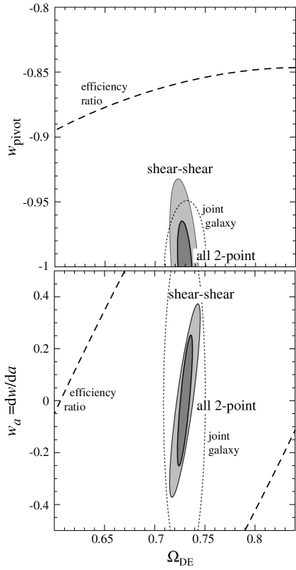
The combined galaxy-shear and galaxy-galaxy power spectra potentially have constraining power that is comparable to the shear-shear spectra. The combination of all three reduces the errors by of order $\sqrt{2}$ or more versus shear alone, leading to marginalized errors of $\sigma(\Omega_{\rm DE})=0.005$, $\sigma(w_{\rm pivot})=0.02$ [$\sigma(w_{0})=0.05$], and $\sigma(w_{a})=0.17$. More importantly they provide important cross checks against shear systematics on the one hand and inadequate halo modeling on the other.

For comparison with other probes, it is useful to note that the dark energy pivot point of the combined power spectra information is $z_{\rm pivot}=0.36\approx z_{\rm DE}$, the epoch of dark energy domination. Equation (44) then maps the errors back into a more conventional description such as $w_{0}$ ($a_{n}=1$). For example if we add in projected CMB constraints for the Planck satellite Planck , the errors improve to $\sigma(\Omega_{\rm DE})=0.004$, $\sigma(w_{\rm pivot})=0.01$ [$\sigma(w_{0})=0.04$], $\sigma(w_{a})=0.08$ as shown in Fig. 4. Note that the combined pivot point shifts to higher redshift. Here we have employed the sensitivities in Hu01c amounting to e.g. $\sigma(\ln D_{*})=0.002$ where $D_{*}$ is the angular diameter distance to last scattering; note that current constraints are at the 0.04 level.

Finally, with all three power spectra one can probe the evolution of the halo parameters and hence aspects of the evolution of the underlying galaxy population. We show in Fig. 5 the resulting errors on the 5 halo parameters as a function of redshift employing all $2$-point information out to $l_{P}=3000$. The errors for different redshifts are nearly independent whereas the errors between the 5 halo parameters at a given redshift are strongly correlated. The correlation indicates degeneracies between the parameters as can also be seen in Fig. 12. Thus there are combinations of halo parameters that are better determined than implied by Fig. 5. These combinations control the shape and amplitude of the spectra. For example, the linear combination that controls the bias and correlation coefficient across the $0.3<z<0.4$ bin and at scales central to the constraint, e.g. $k=0.3h$ Mpc^-1 are separately constrained at the level of $\sigma(\ln b)=0.01$ and $\sigma(\ln R)=0.004$ (fiducial values: $b=2.2$ and $R=1.2$). Constraints on the correlation coefficient mainly reflect its insensitivity to halo parameters on large scales; they weaken in the deeply non-linear regime. Constraints on the bias as a function of scale remain at the percent level from the linear to well into the non-linear regime.

Figure 5: Halo parameter errors as a function of redshift for the $N_{L}=10$ lens galaxy bins and $N_{S}=5$ source galaxy bins with all 2-point information to $l_{P}=3000$ and the efficiency ratio on all scales. Parameters at different redshifts are largely uncorrelated whereas those at the same redshift are highly correlated. Linear combinations that control the shape and amplitude of the power spectra are better constrained (see text).

IV Discussion

The joint analysis of galaxy clustering and lensing data from next-generation surveys offers unique opportunities to simultaneously determine the evolution of clustering in the dark matter and galaxies. These surveys are expected to provide multi-color catalogs of galaxies with well characterized photometric redshifts well beyond $z=1$. We have shown here that with redshift information, even at the 2-point or power spectrum level, there is enough information in the galaxy-shear correlation, especially when combined with galaxy-galaxy correlations, to jointly solve for a model with $\sim 50$ parameters to describe the galaxy evolution and $3$ dark energy parameters. We have conservatively allowed the galaxy parameters to vary independently as a function of lens redshift and marginalized the associated parameters when quoting dark energy constraints.

The dark energy parameter determinations are statistically competitive with the shear-shear correlations and should be more robust to systematic errors in the shear determinations. They furthermore can provide a better redshift localization of dark energy effects given the broad lensing kernel of the shear.

These determinations are assisted by two relatively robust features in the halo model: on large scales, the combination of galaxy-mass correlations and galaxy-galaxy correlations may be used to determine the underlying mass-mass correlations in a manner that is only weakly sensitive to halo model assumptions; on small scales the ratio of galaxy-shear correlations at different source redshifts yields distance ratio information that is only weakly dependent on the evolution of the galaxy-mass correlation.

Equally important, by combining galaxy-galaxy and galaxy-shear clustering one can determine whether the halo model employed here suffices as a description of the relationship between galaxies and dark matter halos. Consistency of the halo determinations can also be checked by selecting lens galaxies with multiple cuts on luminosity or rarity. Consistency of the dark energy determinations can be checked against the shear-shear correlations which depend only on the mass spectrum. A further extension to include contributions from the many galaxy-shear bispectra would also improve parameter accuracies and provide cross-checks Hui99 ; TakJai03 .

Halo model parameter determinations will be valuable in testing models of galaxy formation (e.g. Beretal03 ; Scr03 ; Zehetal03 ). Galaxy parameters measured from surveys as a function of galaxy type, luminosity and redshift can be compared with simulations and semi-analytic model predictions of the same parameters. Although these studies may show that the our halo model requires further modification and extension, we believe that the prospects are bright for a joint solution of galaxy and dark matter clustering.

Acknowledgments: We thank G. Bernstein, D. Holz, A. Kravtsov, M. Takada, A. Tasitsiomi and especially E. Sheldon for many useful discussions. W.H. is supported by NASA NAG5-10840, the DOE, and the Packard Foundation. B.J. is supported by NASA NAG5-10923 and the Keck Foundation.

Appendix A Cosmological Power Spectrum

The linear mass power spectrum $P(k)$ which underlies all observable power spectra depends only on well-motivated cosmological parameters in the context of the successful $\Lambda$CDM cosmology. In this section, we describe its parameterization in terms of the initial conditions §A.1 and evolution §A.2.

A.1 Initial Conditions

We begin by assuming that massive neutrinos make a negligible contribution to the matter density. The shape of the mass power spectrum is then specified by the baryon density $\Omega_{b}h^{2}$, the dark matter density $\Omega_{m}h^{2}$, and the spectrum of initial curvature fluctuations $\zeta$

$$\Delta_{\zeta}^{2}=\delta_{\zeta}^{2}\left({k\over k_{0}}\right)^{n-1}\,,$$ (34)

where $k_{0}=0.05$ Mpc^-1 is the normalization scale. We take fiducial values for these parameters that are consistent with the WMAP determinations: $\Omega_{b}h^{2}=0.024$, $\Omega_{m}h^{2}=0.14$, $n=1$ and $\delta_{\zeta}=5.07\times 10^{-5}$ Speetal03 . The current uncertainties in these parameters are at the 10% level or better. Note that $\delta_{\zeta}$ is related to the WMAP normalization parameter by

$$A=(1.84\delta_{\zeta}\times 10^{4})^{2}\,,$$ (35)

and current and future uncertainties in this parameter are expected to be dominated by uncertainties in the Thomson optical depth to reionization $\tau$, i.e.

$$\delta_{\zeta}\approx 5.07e^{-(0.17-\tau)}\times 10^{-5}.$$ (36)

Thus the power spectrum as a function of $k$ in Mpc^-1 (not $h$ Mpc^-1) in the matter dominated regime can be considered as largely known.

A.2 Evolution

The shape of this initial power spectrum does not change during dark energy domination on scales below the sound horizon of the dark energy. The amplitude of the linear power spectrum depends on the initial normalization $\delta_{\zeta}$ and the “growth function”, here the decay rate of potential fluctuations $G$

$$P(k,z)=\left[{1\over{1+z}}{G(z)\over G_{0}}\right]^{2}P(k,0)\,,$$ (37)

where $G_{0}\equiv G(z=0)$ and we assume that all relevant scales are sufficiently below the maximal sound horizon of the dark energy. $P(k,0)$ can be evaluated from any one of a number of Einstein-Boltzmann codes.

The normalization of the linear power spectrum today is conventionally given at a scale of $r=8h^{-1}$Mpc

$$\sigma_{8}^{2} \equiv \int{d^{3}k\over(2\pi)^{3}}P(k,0)W_{\sigma}^{2}(kr)$$

$$\sigma_{8} \approx {\delta_{\zeta}\over 5.59\times 10^{-5}}\left({\Omega_{b}h^{2}\over 0.024}\right)^{-1/3}\left({\Omega_{m}h^{2}\over 0.14}\right)^{0.563}$$ (38)

$$\times(3.123h)^{(n-1)/2}\left({h\over 0.72}\right)^{0.693}{G_{0}\over 0.76}\,,$$

where $W_{\sigma}(x)=3x^{-3}(\sin x-x\cos x)$ is the Fourier transform of a top hat window. The approximation in Eqn. (38) is valid to the 1% level for individual variations of the parameters in the regime $0.019\leq\Omega_{b}h^{2}\leq 0.03$, $0.11\leq\Omega_{m}h^{2}\leq 0.18$, $0.7\leq n\leq 1.3$, $0.5\leq h\leq 1$ which more than span the current observational errors. Note that because the normalization is given in $h^{-1}$ Mpc, there is a strong scaling with the Hubble constant. This scaling actually assists dark energy determinations since in a flat universe $\Omega_{\rm DE}=1-\Omega_{m}$ and precise measurements of $\Omega_{m}h^{2}$ makes $h$ depend on $\Omega_{\rm DE}$ only. A measurement of the Hubble constant is a measurement of the dark energy density. Likewise a measurement of $\sigma_{8}$ is a measurement of a specific combination of dark energy parameters.

We will hereafter limit ourselves to flat universes but correspondingly neglect the dark energy information from the CMB unless otherwise specified. The angular diameter distance to recombination $D_{*}$ has been measured to $\sigma(\ln D_{*})=0.04$ Speetal03 and this constraint will continue to improve with better measurements of $\Omega_{m}h^{2}$ from the peaks as (see e.g. HuFukZalTeg00 )

$$\sigma(\ln D_{*})\approx{1\over 4}\sigma(\ln\Omega_{m}h^{2})\,.$$ (39)

The rationale behind dropping this constraint is that this measurement will be used in conjunction with galaxy and lensing constraints to eliminate any small curvature contribution that might exist. In a flat universe, $D_{*}$ closely follows $G_{0}$ in its dark energy dependence and so may be used as a powerful consistency test for the absence of spatial curvature. We discuss this issue further in §III.3.

The growth function $G$ then depends only on the dark energy density $\Omega_{{\rm DE}}(a)=8\pi G\rho_{\rm DE}/3H^{2}$ and equation of state $w(a)=p_{\rm DE}/\rho_{\rm DE}$ through the equation (e.g. Hu01c )

$$\frac{d^{2}G}{d\ln a^{2}} + \left[\frac{5}{2}-\frac{3}{2}w(a)\Omega_{{\rm DE}}(a)\right]\frac{dG}{d\ln a}$$ (40)

$$+ \frac{3}{2}[1-w(a)]\Omega_{{\rm DE}}(a)G=0\,,$$

where the initial conditions are $G=1$ and $dG/d\ln a=0$ at an epoch well before dark energy domination $z\gg z_{\rm DE}$,

$$1+z_{\rm DE}=a_{\rm DE}^{-1}\approx\left({\Omega_{\rm DE}\over{1-\Omega_{\rm DE}}}\right)^{-1/3w_{0}}\,,$$ (41)

where $\Omega_{\rm DE}\equiv\Omega_{\rm DE}(z=0)$ and $w_{0}\equiv w(z=0)$.

Given a constant equation of state, $G_{0}$ follows the approximate form

$$G_{0} \approx 0.76\left({\Omega_{m}\over 0.27}\right)^{0.236}F[\Omega_{\rm DE}^{4/3}(1+w_{\rm DE})]\,,$$

$$F(x) = (1+0.498x+4.88x^{3})^{-1}\,,$$ (42)

where the approximation holds to $\sim 1\%$ for separate variations of $-1<w_{\rm DE}<-1/2$ and $0.12<\Omega_{m}<0.5$. Here and throughout we denote a dark energy parameterization for which $w$ is constant with $w_{\rm DE}=w$. Note the fairly strong scaling of $G_{0}$ with $w_{\rm DE}$ around the fiducial model $\Delta G_{0}/G_{0}\approx-0.33\Delta w_{\rm DE}$.

A dynamical form of dark energy is unlikely to possess a strictly constant equation of state. Since it only has observable consequences at $z\lesssim z_{\rm DE}$, it is convenient to describe the function with its first order Taylor expansion. We therefore choose an equation of state parameterization

$$w(a)=w_{n}+(a_{n}-a)w_{a}\,,$$ (43)

with the expansion around some epoch $a_{n}$; this generalizes the form employed in Lin03 where $a_{n}=1$.

We instead choose $a_{n}=a_{\rm pivot}$ such that the errors in $w_{\rm pivot}$ and $w_{a}$ for a given observable are uncorrelated $C_{w_{\rm pivot}w_{a}}=0$. The pivot point $a_{\rm pivot}$ can be derived from a general representation via the transformation

$$C_{\mu\nu}^{\prime}=\sum_{\alpha\beta}{\partial p_{\alpha}^{\prime}\over\partial p_{\mu}}C_{\alpha\beta}{\partial p_{\beta}^{\prime}\over\partial p_{\nu}}\,.$$ (44)

For the transformation to the pivot representation EisHuTeg99b

$${\partial w_{\rm pivot}\over\partial w_{n}}=1,\qquad{\partial w_{\rm pivot}\over\partial w_{a}}=a_{n}-a_{\rm pivot}\,,$$ (45)

from which it follows that the errors decorrelate for a shift in the pivot of

$${a_{n}-a_{\rm pivot}}=-{C_{w_{n}w_{a}}\over C_{w_{a}w_{a}}}\,.$$ (46)

Moreover the resulting errors on $w_{\rm pivot}$ are then equal to those on $w_{\rm DE}$, a constant $w$. The pivot redshift is therefore also the redshift at which $w$ is best constrained.

The drawback to choosing the pivot redshift is that it is specific to the observable, survey and dark energy model. As the redshift where the dark energy evolution is best constrained, the pivot point for growth measurements tends to coincide roughly with $z_{n}\approx 0.4$ or $z_{\rm DE}$ in the fiducial $\Lambda$ model. In fact, further taking $w_{\rm DE}\rightarrow w(a_{\rm DE})$ in Eqn. (42) yields an approximation to the growth function that is good to several percent across a wide range of $w_{a}$. Choosing this standard normalization epoch then provides the benefits of the pivot point without the drawbacks. Although we will employ the pivot redshift for the galaxy-lensing study below, it is sufficiently close to $z_{\rm DE}$ that it may be interpreted in this manner. Note that the pivot point for distance-based dark energy measurements can be at even higher redshift $z_{\rm DE}\lesssim z\lesssim 1$ so that it becomes even more important to choose a $z_{n}\neq 0$ for the characterization of constraints.

In summary, our linear matter power spectrum is specified by $7$ parameters: 4 that are already well constrained by the CMB $\delta_{\zeta}(=5.07\times 10^{-5})$, $n(=1)$, $\Omega_{b}h^{2}(=0.024)$, $\Omega_{m}h^{2}(=0.14)$, and 3 dark energy parameters $\Omega_{\rm DE}(=0.73)$, $w_{\rm pivot}(=-1)$ (or $w_{0}$), $w_{a}(=0)$ which galaxy-lensing power spectra can help constrain. Parameter values of the fiducial cosmology are given in parentheses. Given a linear power spectrum and cosmology, cosmological simulations can accurately predict the fully non-linear mass power spectrum and hence the shear-shear 2-point correlations. On the other hand, the power spectra involving galaxies will require some semi-analytic modeling for the foreseeable future. We now turn to a halo model for the parameterization of the underlying relationship between the observable power spectra and the linear theory predictions.

Figure 6: Host halo mass function $dn_{h}/d\ln M_{h}$ and halo occupation distribution function $\bar{N}_{g}(M_{h})$. Three halo parameters control the shape of the distribution: $A_{s}$ the satellite-host normalization or crossing point, $m_{s}$ the satellite slope (which pivots $\bar{N}_{s}$ about the crossing point), and $\sigma_{\ln M}$ the scatter in the mass observable relation. Galaxies selected by a flux limit are matched in number density by adjusting the threshold mass $M_{\rm th}$, here illustrated for $M_{\rm th}=10^{13.5}h^{-1}M_{\odot}$. Here and throughout the fiducial model is a flat $\Lambda$CDM model with cosmological parameters $\Omega_{m}=0.27$, $h=0.72$, $n_{s}=1$, $\delta_{\zeta}=5.07\times 10^{-5}$ ($\sigma_{8}=0.91$) and $\Omega_{b}h^{2}=0.024$ and halo parameters $A_{s}=30$, $m_{s}=1$ and $\sigma_{\ln M}=0.1$.

Appendix B Halo Model

To study the information contained in the lensing and galaxy two point observables, we require a model for the underlying three dimensional galaxy and mass density power spectra. Recent work on comparing simulations to galaxy clustering data have shown that to first approximation, galaxies selected on luminosity are assigned to a mass-based selection of dark matter (sub)halos of the same spatial number density Kraetal03 . This mapping avoids the traditional problem of defining explicit halo mass-luminosity relationships. In §B.1, we build this underlying ansatz into a halo description of the galaxies and mass (see CooShe02 for a review) and obtain a parameterized model for their joint power spectra in §B.2. We then describe the phenomenology of the fiducial halo model in §B.3 and study the sensitivity of the power spectra to variations in the halo model and cosmological parameters in §B.4.

B.1 Host and Satellites

Under the halo model, the power spectra are described by the abundance, clustering, density profile, substructure and galaxy occupation of dark matter halos. For the comoving abundance of host halos, we take the mass function SheTor99

$${dn_{h}\over d\ln M}={\rho_{0}\over M}f(\nu){d\nu\over d\ln M}\,,$$ (47)

where $\rho_{0}$ is the matter density today $\rho_{0}=\rho_{m}(z=0)$, $\nu=\delta_{c}/\sigma$

$$f(\nu)=A\sqrt{{2\over\pi}a\nu^{2}}[1+(a\nu^{2})^{-p}]\exp[-a\nu^{2}/2]\,.$$ (48)

Here $\sigma(M;z)$ is the rms of the linear density field smoothed with a top hat of a radius that encloses the mass $M$. We choose $\delta_{c}=1.69$, $a=0.75$, $p=0.3$, and $A$ such that $\int d\nu f(\nu)=1$. The mass function of the fiducial model is shown in Fig. 6 bracketing the redshifts of interest for lensing ($0<z<1$).

The halo clustering is then given by the peak-background split as Kai84b ; MoWhi96

$$b(M)=1+{a\nu^{2}-1\over\delta_{c}}+{2p\over\delta_{c}[1+(a\nu^{2})^{p}]}\,.$$ (49)

For the halo density profile, we take the NFW form NavFreWhi97

$$\rho(r,M,c)={\Delta_{v}\rho_{0}\over 3}{c^{3}\over\ln(1+c)-c/(1+c)}{1\over Rc(1+Rc)^{2}}\,,$$ (50)

where $R=r/r_{v}$ with the virial radius

$$r_{v}=\left({3M_{v}\over 4\pi\rho_{0}}\right)^{1/3}\,.$$ (51)

We take the concentration Buletal01

$$c(M_{v})={9\over{1+z}}\left({M_{v}\over M_{*}}\right)^{-0.13}\,,$$ (52)

where $M_{*}$ is defined by $\sigma(M_{*};z=0)=\delta_{c}$. We convert between the halo mass $M$, assumed to be defined at an overdensity of 180 times the mean density, and the virial mass $M_{v}$ defined at an overdensity BryNor98

$$\Delta_{v}(z)={18\pi^{2}+82\Omega_{\rm DE}(z)-39[\Omega_{\rm DE}(z)]^{2}\over 1+\Omega_{\rm DE}(z)}\,,$$ (53)

using the NFW profile (see e.g. HuKra02 ).

Figure 7: Satellite fraction $dn_{s}/d(n_{h}+n_{s})$. The satellite fraction at a given mass for a given halo occupation distribution $N(M_{h})$ is largely a function of the peak height threshold $\nu$ in Eqn. (47) as rare objects are unlikely to be satellites. The conversion to mass at $z=0$ is given in the upper axis. The range of fractions for $M=10^{13.5}h^{-1}M_{\odot}$ and $0<z<1$ is shown shaded.

The profile enters into the power spectra through its normalized Fourier transform

$$y(k,M,c)={1\over M}\int_{0}^{r_{v}}dr4\pi r^{2}\rho(r,M,c){\sin(kr)\over kr}\,.$$ (54)

Although there are current uncertainties in these descriptions of the halo mass function, bias and concentration, we choose not to associate free parameters with these dark matter clustering properties. The characterization of these properties and more importantly the mass power spectrum itself can in principle be fixed by better simulations. Similarly for the association with galaxies, since we will be matching number densities of objects, the halo mass definition employed here may be replaced with any variable that defines the selection of objects in the simulations and is a monotonic function of galaxy luminosity on average.

The halo model predicts the galaxy and galaxy-mass power spectra under an assumption for the statistics of the occupation of the host halo by galaxies Sel00 ; SheJai03 . Since each galaxy also carries its own dark matter halo we will hereafter distinguish between the host halo of mass $M_{h}$ and its satellite halos of mass $M_{s}$. For simplicity we take the satellites to also have NFW profiles but with an adjustable concentration; a more sophisticated model would account for the change in the functional form due to truncation from tidal stripping and trends in mass.

Figure 8: Relative galaxy-galaxy and galaxy-mass power spectra. In the linear regime, $k<0.1h$ Mpc^-1, both $b=(P^{{\delta_{g}\delta_{g}}}/P^{{\delta_{m}\delta_{m}}})^{1/2}$ and $b/R=P^{{\delta_{g}\delta_{g}}}/P^{{\delta_{g}\delta_{m}}}$ return the linear bias which increases as the objects become rarer. In the non-linear regime, $P^{{\delta_{g}\delta_{g}}}$ and $P^{{\delta_{g}\delta_{m}}}$ continue to track each other and exceed the mass power spectrum.

We begin by taking a simulation-motivated universal form for the number of dark matter satellites in the host halo as a function of their mass ratio TorDiaSye98 ; Ghietal00

$${d\bar{N}_{s}\over d\ln M_{s}}=m_{s}\left({M_{h}\over A_{s}M_{s}}\right)^{m_{s}}$$ (55)

for $M_{h}/(100A_{s})\leq M_{s}\leq M_{h}$ where simulations suggest that $A_{s}\approx 30$ and $m_{s}\approx 1$ Kraetal03 . The cutoff to low masses prevents a mild logarithmic divergence in the total mass; this arbitrary cutoff only affects the mass power spectrum at unobservably small scales.

We next associate galaxies with these satellites. The total number of satellite galaxies above a given threshold mass $M_{\rm th}$ then becomes

$$\bar{N}_{s} = \int_{M_{\rm th}}^{\infty}{dM_{s}\over M_{s}}{d\bar{N}_{s}\over d\ln M_{s}}$$ (56)

$$= \left({M_{h}\over A_{s}M_{\rm th}}\right)^{m_{s}}\,.$$

To this population of satellite galaxies we add the central galaxy associated with the host halo itself to obtain the total number of galaxies above the threshold (see Fig. 6)

$$N_{g}(M_{h};M_{\rm th})=N_{h}+N_{s}\,.$$ (57)

These two pieces have different statistical properties. The central galaxy may be either above or below threshold and hence either occupied or unoccupied leading to $\langle N_{h}^{p}\rangle=\langle N_{h}\rangle=\bar{N}_{h}$. We model the average value as a step function at some limiting mass $M_{\rm th}$ smoothed by a Gaussian in $\ln M_{h}$ to reflect scatter in the conversion of a magnitude limit to a mass limit

$$\bar{N}_{h}={1\over 2}{\rm Erfc}\left({\ln M_{\rm th}/M_{h}}\over\sqrt{2}\sigma_{\ln M}\right)\,.$$ (58)

The dark matter satellites follow a Poisson distribution with $\langle N_{s}^{2}\rangle=\bar{N}_{s}^{2}+\bar{N}_{s}$ Kraetal03 .

Given a fixed shape for $\bar{N}_{g}$, the threshold mass $M_{\rm th}$ is not a free parameter. Rather it is fixed by matching the space density of galaxies to the space density inferred by the observed number counts

$$\bar{n}_{V}(z;M_{\rm th}) = \int_{0}^{\infty}{dM_{h}\over M_{h}}\bar{N}(M_{h};M_{\rm th}){dn_{h}\over d\ln M_{h}}$$ (59)

$$= \bar{n}_{A}W_{g}(z)\,.$$

Note that by choosing rare objects, the implied $M_{\rm th}>M_{*}$ and so the population will be dominated by host galaxies rather than satellite galaxies (see Fig. 6). This fact will be useful in minimizing the uncertainties and systematic errors associated with the model for $\bar{N}_{s}$ and the satellite profiles, e.g. the mass scaling of the concentration parameters. The satellite contribution can be quantified by considering the satellite mass function

$${dn_{s}\over d\ln M_{s}} = \int_{M_{s}}^{\infty}{dM_{h}\over M_{h}}{d\bar{N}_{s}\over d\ln M_{s}}{dn_{h}\over d\ln M_{h}}$$ (60)

$$= \int_{M_{s}}^{\infty}{dM_{h}\over M_{h}}m_{s}\left({M_{h}\over A_{s}M_{s}}\right)^{m_{s}}{dn_{h}\over d\ln M_{h}}$$

and comparing it to the host halo mass function itself

$${dn_{s}\over d(n_{h}+n_{s})}\equiv{dn_{s}\over d\ln M}\left[{d(n_{s}+n_{h})\over d\ln M}\right]^{-1}\,.$$ (61)

This ratio depends mainly on the peak height threshold $\nu$ for a given form for the shape of $\bar{N}_{g}(M_{h})$ (see Fig. 7). With our fiducial choice, it saturates at the low mass end at $\sim 30\%$. With a selection of rare objects, e.g. corresponding to $M_{\rm th}\approx 10^{13.5}h^{-1}M_{\odot}$ in the fiducial model, the satellite fraction can be less than $10\%$ at all redshifts.

Figure 9: Correspondence of spatial wavenumber $k$ ($h^{-1}$ Mpc) to angular wavenumber $l$ as a function of redshift $z$ given by the Limber approximation in the fiducial cosmology. Also shown is the projected non-linear scale $k_{\rm nl}$ where $k^{3}P^{{\delta_{m}\delta_{m}}}/2\pi^{2}=1$. Note that $l\sim 10^{3}$ corresponds to the mildly non-linear regime for the redshifts in question.

B.2 Power Spectra

The power spectra are defined by the host and satellite distributions as

$$P^{\delta_{m}\delta_{m}}(k) = I_{1m}^{2}(k)P(k)+I_{2m}(k)\,,$$

$$P^{\delta_{g}\delta_{g}}(k) = I_{1g}^{2}(k)P(k)+I_{2g}(k)\,,$$

$$P^{\delta_{g}\delta_{m}}(k) = I_{1g}(k)I_{1m}(k)P(k)+I_{2c}(k)\,.$$ (62)

The indices $1$ and $2$ refer to the number of points in a single halo. The first piece then represents two points in separate host halos correlated by the linear power spectrum $P(k)$

$$I_{1m} = \int{dM_{h}\over M_{h}}\left({M_{h}\over\rho_{0}}\right){dn_{h}\over d\ln M_{h}}b(M_{h})y_{h}\,,$$ (63)

$$I_{1g} = {1\over\bar{n}_{V}}\int{dM_{h}\over M_{h}}[\bar{N}_{h}+\bar{N}_{s}y_{g}]{dn_{h}\over d\ln M_{h}}b(M_{h})\,,$$

and the second piece is the contribution from two points within a parent halo including its satellite contributions

$$I_{2m} = \int{dM\over M}\left({M\over\rho_{0}}\right)^{2}\left[{dn_{h}\over d\ln M}y^{2}_{h}+{dn_{s}\over d\ln M}y^{2}_{s}\right]\,,$$

$$I_{2g} = {1\over\bar{n}_{V}^{2}}\int{dM\over M}[\bar{N}_{s}^{2}y_{g}^{2}+2\bar{N}_{h}\bar{N}_{s}y_{g}]{dn_{h}\over d\ln M}\,,$$

$$I_{2c} = {1\over\bar{n}_{V}}\int{dM\over M}\left({M\over\rho_{0}}\right)\Big{[}{dn_{h}\over d\ln M}(\bar{N}_{h}y_{h}+\bar{N}_{s}y_{h}y_{g})$$ (64)

$$+{dn_{s}\over d\ln M}H(M-M_{\rm th})y_{s}\Big{]}\,,$$

Here we have employed the shorthand convention $y_{h,s}\equiv y(k,c_{h,s},M_{h,s})$, $y_{g}=y(k,c_{g},M_{h})$ and the step function $H(x)=1$ for $x\geq 0$ and $H(x)=0$ for $x\leq 0$. The effect of satellite galaxies occupying satellite halos takes the same form as the central galaxy occupying the host halo GuzSel02 except that we have neglected the small effect of smoothing around the threshold mass. In this description, the satellite-satellite mass correlation and satellite-halo mass correlation are implicitly included as the replacement of mass lost to subhalos in the term involving the parent profiles $y_{h}$ in Eqn. (64).

Figure 10: Angular power spectra in the fiducial halo and cosmological model for two galaxy ($g_{1}:0<z<0.5$; $g_{2}:0.5<z<1$; $M_{\rm th}=10^{13.5}h^{-1}M_{\odot}$) and source bins ($\epsilon_{1}:z<1.5$; $\epsilon_{2}:z>1.5$; $z_{{\rm med};S}=1.5$). Note the inflection at $l\sim$ few $\times 10^{2}$ and the large number of cross spectra $(N_{L}N_{S}=4)$.

B.3 Fiducial Model

Five functions of redshift specify our halo model, the satellite-host normalization $A_{s}$, the slope of the satellite mass function and occupation distribution $m_{s}$, the scatter in the mass observable relation $\sigma_{\ln M}$, the concentration of the satellites in the host halo $c_{g}$ and the concentration of the mass profiles of the satellites $c_{s}$. We assume that the latter two follow the mass scaling of isolated halos in Eqn. (52) but have an arbitrary normalization. We further represent the functions by a set of $5N_{L}$ parameters that specify their values at the redshifts of the $N_{L}$ lens redshift bins.

Figure 11: Tangential shear and surface mass density difference in the fiducial halo and cosmological model for several choices of the mass threshold. Here we take a delta function distribution of lenses ($z_{L}=0.5$) and sources ($z_{S}=1.5$). Note the turnover on small scales ($0.5-1^{\prime}$) and inflection near $10^{\prime}$ causing excess signal at large angles.

The values of these parameters will in the future be determined by fitting to the joint power spectra. However, to study the potential of these future data sets we must specify their values in the fiducial model. The sensitivity of observables to variations in their values around this model is then quantified through the Fisher matrices of §II.3.

We choose fiducial values that are roughly consistent with low redshift measurements from the SDSS lensing data Sheetal03 and $N$-body simulations: $A_{s}=30$, $m_{s}=1$, $\sigma_{\ln M}=0.1$ for all redshift bins. These three parameters define the shape of $\bar{N}_{g}$ shown in Fig. 6. In our fiducial model the concentration parameters $c_{s}=c_{g}=c_{h}$.

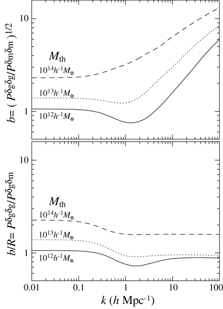
In Fig. 8, we show the galaxy-galaxy and galaxy-mass power spectra with the fiducial halo and cosmological parameters. They are shown relative to the mass-mass spectrum at $z=0$ for halo abundances corresponding to several different mass thresholds in the fiducial $\Lambda$CDM cosmology (see §A). In the linear regime $k<0.1h$ Mpc^-1 the ratios

$$b(k)\equiv\left({P^{{\delta_{g}\delta_{g}}}\over P^{{\delta_{m}\delta_{m}}}}\right)^{1/2}$$ (65)

and

$${b(k)\over R(k)}\equiv{P^{{\delta_{g}\delta_{g}}}\over P^{{\delta_{g}\delta_{m}}}}$$ (66)

both return the constant linear bias of the objects. In other words, in the linear regime the correlation coefficient

$$R(k)\equiv{P^{{\delta_{g}\delta_{m}}}\over(P^{{\delta_{g}\delta_{g}}}P^{{\delta_{m}\delta_{m}}})^{1/2}}\approx 1$$ (67)

independent of the population or halo model parameters. In this regime, a measurement of $P^{{\delta_{g}\delta_{m}}}$ and $P^{{\delta_{g}\delta_{g}}}$ is a measurement of the mass power spectrum $P$ and hence in combination can be used to study the dark-energy dependent growth rate. The linear bias increases with the mass threshold $M_{\rm th}$ or more generally with the rarity of the objects.

Figure 12: Halo parameter sensitivity compared with dark energy sensitivity of galaxy-galaxy and galaxy-mass power spectra. In the non-linear regime, galaxy-galaxy power spectra become highly sensitive to most halo parameters. Galaxy-galaxy power spectra are insensitive to dark energy effects on the growth rate since a lowering of the amplitude is compensated by an increase in bias due to the increased rarity of the objects. Conversely the galaxy-mass power spectra are less sensitive to halo parameters and more sensitive to the dark energy.

In the non-linear regime, the bias becomes strongly scale dependent reflecting the correlations within a parent halo. On the other hand, the ratio $b/R$ remains remarkably constant Sel00 . Formally the combination indicates that the galaxy-mass correlation $R>1$. Under the halo model, every galaxy has a dark matter halo around it and so the relevant power spectrum for computing the correlation coefficient is corrected for the excess shot noise power $P^{{\delta_{g}\delta_{g}}}+\bar{n}_{V}^{-1}$. The scale dependence of $b$ and $b/R$ can be used to pin down the halo parameters. For fixed halo parameters, it marks the non-linear scale which also depends on the dark energy through the linear growth rate.

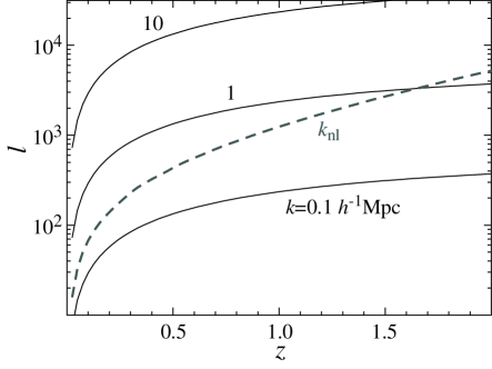
These properties remain qualitatively true for angular power spectra with the caveat that projection effects can broaden the non-linear transition regime for wide redshift shells for the lens galaxies and the broad efficiency for lensing. In Fig. 9 we show the correspondence of $k$ and $l$ in the fiducial cosmology and under the Limber approximation. In Fig. 10, we show an example of the Limber projection to the angular power spectra. Note that the inflection caused by the transition between the one host halo and (linear) two host halo regimes occurs at wavenumbers of $l\sim{\rm few}\times 10^{2}$. Note that there are $N_{L}=2$ galaxy spectra, $N_{L}N_{S}=4$ cross spectra, and $N_{S}(N_{S}+1)/2=3$ shear spectra.

In Fig. 11, we highlight the one halo regime by showing the predictions for the tangential shear from Eqn. (15) for a given source and lens configuration. Note that the shear turns over as the angular radius resolves the scale radius of the halo and shows another break on large scales marking the beginning of the two halo regime.

B.4 Parameter Sensitivity

The sensitivity of the power spectra to halo and cosmological parameters is quantified by their derivatives with respect to the parameters in Eqn. (25). In Fig. 12 we compare the halo parameter sensitivity of galaxy-galaxy and galaxy-mass spectra to the equation of state parameter $w_{\rm DE}$ at $z=0$ for a population with an abundance in the fiducial model corresponding to $M_{\rm th}=10^{13.5}h^{-1}M_{\odot}$. Since the initial normalization of the power spectrum is here fixed, sensitivity to $w_{\rm DE}$ is equivalent to sensitivity to the present-day normalization $\sigma_{8}$ (see Eqn. (42)).

The galaxy-galaxy spectrum is strikingly insensitive to $w_{\rm DE}$ compared with the halo parameters that control $N_{g}(M_{h})$: $A_{s}$, $m_{s}$ and $\sigma_{\ln A}$. Changes in the parameters that control its shape change the power spectrum on all scales since they enter into the calculation of the mass threshold $M_{\rm th}$ and hence the bias of the host halos. A change in the cosmology that for example lowers the present amplitude of the matter power spectrum makes galaxies of a given number density rarer. Since rarer objects are more highly biased tracers of the matter, the galaxy-galaxy power spectrum remains largely unchanged. The same is not true for the galaxy-mass power spectra. Indeed the galaxy-mass power spectra are substantially more sensitive to cosmological parameters than halo parameters. The combination of galaxy-galaxy and galaxy-mass power spectra is then particularly powerful for simultaneously determining the halo and cosmological parameters.

Neither set of spectra are very sensitive to the concentration parameters $c_{s}$ and $c_{g}$ except at very $k$ values that correspond to $l\gg 10^{3}$ for the redshifts in question (see Fig. 9). By definition, the concentration parameters only affect the power spectrum on small scales. Furthermore since we have chosen a high mass threshold, the fraction of objects that are satellites and hence affected by these parameters is low. This insensitivity helps justify our crude treatment of the profiles.

Variable	Definition	Eq.
$N_{L}$	Lens galaxy bins	(28)
$N_{S}$	Source galaxy bins	(28)
$N_{h}$	Host halo occupation	(57)
$N_{s}$	Satellite halo occupation	(56)
$N_{g}$	Total halo occupation	(57)
$M$	Halo mass	(47)
$M_{h}$	Host halo mass	(55)
$M_{s}$	Satellite halo mass	(55)
$M_{v}$	Virial mass	(51)
$\hat{\bf n}$	Angular position	(2)
$n$	Initial tilt	(34)
$n_{A}$	Galaxy angular density	(8)
$n_{V}$	Galaxy space density	(7)
$n_{h}$	Host halo space density	(47)
$n_{s}$	Satellite halo space density	(60)
$w$	Dark energy equation of state	(40)
$w_{\rm DE}$	Constant $w(a)$	(42)
$w_{n}$	Specific epoch $w(a_{n})$	(43)
$w_{\rm pivot}$	Best constrained $w(a_{\rm pivot})$	(45)
$w_{0}$	Present day $w(a=1)$	(41)
$w_{a}$	Evolution $-dw/da$	(43)

Table 1: Easily confused variables.

As for the mass-mass power spectrum, and hence the shear-shear power spectrum, it is of course the most sensitive to the dark energy parameters being directly related to the linear growth function of Eqn. (40). It formally also depends on the satellite mass function and hence the halo model parameters that control it. However we here take the perspective that the form of the mass-mass power spectrum as a function of cosmology will in the future be fixed directly by simulations replacing the halo model description. Hence we take the uncertainties in the halo parameters to only affect the galaxy-galaxy and galaxy-mass power spectra. Operationally we assume that variations in $P^{{\delta_{m}\delta_{m}}}$ due to the variations in the satellite mass function are localized to the galaxy mass regime and compensated by variations at other masses to leave the spectrum invariant. This corresponds to dropping the parameter derivative terms in the Fisher matrix (24).

We provide a guide to easily confused variables in Tab. 1.

References

- (1)
- (2) T.G. Brainerd, R.D. Blandford and I. Smail, Astrophys. J, 466, 623 (1996).
- (3) J.A. Tyson, F. Valdes, J.F. Jarvis and A.P. Mills, Astrophys. J, 281, 59 (1984).
- (4) H. Hoekstra, et al. Astrophys. J, 577, 604 (2002).
- (5) D.R. Smith, G.M. Bernstein, P. Fisher and M. Jarvis, Astrophys. J, 551, 643 (2001).
- (6) P. Fischer, et al. Astron. J., 120, 1198 (2000).
- (7) T. McKay, et al. Astrophys. J, 571, 85 (2002).
- (8) E.S. Sheldon, et al. Astron. J., submitted, astro-ph/0313036 (2003).
- (9) U. Seljak, Mon. Not. R. Astron. Soc., 318, 203 (2000).
- (10) J. Guzik and U. Seljak, Mon. Not. R. Astron. Soc., 321, 439 (2001).
- (11) J. Guzik and U. Seljak, Mon. Not. R. Astron. Soc., 335, 311 (2002).
-
(12)
http://pan-starrs.ifa.hawaii.edu
http://www.dmtelescope.org
http://snap.lbl.gov - (13) A.V. Kravtsov, et al. Astrophys. J, submitted, astro-ph/0308519 (2003).
- (14) D. Limber, Astrophys. J, 119, 655 (1954).
- (15) N. Kaiser, Astrophys. J, 388, 272 (1992).
- (16) G.M. Bernstein and B. Jain, Astrophys. J, in press, astro-ph/0309332 (2003).
- (17) W. Hu and M. White, Astrophys. J, 554, 67 (2001).
- (18) U.L. Pen, Mon. Not. R. Astron. Soc., 346, 619 (2003).
- (19) N. Kaiser and G. Squires, Astrophys. J, 404, 441 (1993).
- (20) R. Scoccimarro, M. Zaldarriaga and L. Hui, Astrophys. J, 527, 1 (1999).
- (21) M. White and W. Hu, Astrophys. J, 537, 1 (2000).
- (22) D.J. Eisenstein and M. Zaldarriaga, Astrophys. J, 546, 2 (2001).
- (23) Y.S. Song and L. Knox, Phys. Rev. D, submitted, astro-ph/0312175 (2003).
- (24) W. Hu, Astrophys. J Lett., 522, 21 (1999).
- (25) D.N. Spergel, et al. Astrophys. J, submitted, astro-ph/0302209 (2003).
- (26) R. Link and M.J. Pierce, Astrophys. J Lett., 502, 63 (1998).
- (27) L. Gautret, B. Fort and Y. Mellier, Astron. Astrophys., 353, 10 (2000).
- (28) G. Golse, J.P. Kneib and G. Soucail, Astron. Astrophys., 387, 788 (2002).
- (29) M. Sereno, Astron. Astrophys., 393, 757 (2002).
- (30) B. Jain and A. Taylor, Phys. Rev. Lett., 91, 1302 (2003).
- (31) J. Zhang and L. Hui, A. Stebbins, Astrophys. J, submitted, preprint (2003).
- (32) http://astro.estec.esa.nl/Planck
- (33) D. Huterer, Phys. Rev. D, 65, 063001 (2002).
- (34) W. Hu, Phys. Rev. D, 65, 023003 (2002).
- (35) L. Hui, Astrophys. J, 519, 9 (1999).
- (36) M. Takada and B. Jain, Mon. Not. R. Astron. Soc., submitted, astro-ph/0310125 (2003).
- (37) A.A. Berlind, et al. Astrophys. J, 593, 1 (2003).
- (38) R. Scranton, Mon. Not. R. Astron. Soc., 339, 410 (2003).
- (39) I. Zehavi, et al. Astrophys. J, submitted, astro-ph/0301280 (2003).
- (40) R. Scoccimarro and R.K. Sheth, Mon. Not. R. Astron. Soc., 329, 629 (2002).
- (41) W. Hu, M. Fukugita, M. Zaldarriaga and M. Tegmark, Astrophys. J, 549, 669 (2001).
- (42) E.V. Linder, Phys. Rev. Lett., 90, 130 (2003).
- (43) D.J. Eisenstein, W. Hu and M. Tegmark, Astrophys. J, 518, 2 (1999).
- (44) A. Cooray and R. Sheth, Phys. Rept., 372, 1 (2002).
- (45) R.K. Sheth and B. Tormen, Mon. Not. R. Astron. Soc., 308, 119 (1999).
- (46) N. Kaiser, Astrophys. J, 284, 9 (1984).
- (47) H.J. Mo and S.D.M. White, Mon. Not. R. Astron. Soc., 282, 347 (1996).
- (48) J.F. Navarro, C.S. Frenk and S.D.M. White, Astrophys. J, 490, 493 (1997).
- (49) J.S. Bullock, et al. Mon. Not. R. Astron. Soc., 321, 559 (2001).
- (50) G.L. Bryan and M.L. Norman, Astrophys. J, 495, 80 (1998).
- (51) W. Hu and A.V. Kravtsov, Astrophys. J, 584, 702 (2003).
- (52) R. Sheth and B. Jain, Mon. Not. R. Astron. Soc., 345, 529 (2003).
- (53) D.N. Spergel, et al. Astrophys. J Supp., 148, 175 (2003).
- (54) G. Tormen, A. Diaferio and D. Syer, Mon. Not. R. Astron. Soc., 299, 728 (1998).
- (55) S. Ghigna, et al. Astrophys. J, 544, 616 (2000).