The Application of Photometric Redshifts to the SDSS Early Data Release
Abstract
The Early Data Release from the Sloan Digital Sky survey provides one of the largest multicolor photometric catalogs currently available to the astronomical community. In this paper we present the first application of photometric redshifts to the million extended sources within these data (with 1.8 million sources having ). Utilizing a range of photometric redshift techniques, from empirical to template and hybrid techniques, we investigate the statistical and systematic uncertainties present within the redshift estimates for the EDR data. For we find that the redshift estimates provide realistic redshift histograms with an rms uncertainty in the photometric redshift relation of 0.035 at and rising to 0.1 at . We conclude by describing how these photometric redshifts and derived quantities, such as spectral type, restframe colors and absolute magnitudes, are stored within the SDSS database. We provide sample queries for searching on photometric redshifts and list the current caveats and issues that should be understood before using these photometric redshifts in statistical analyses of the SDSS galaxies.
1 Introduction
From their inception (Koo (1985); Connolly et al. (1995); Gwyn & Hartwick (1996); Sawicki, Lin & Yee (1997); Hogg et al. (1998); Wang, Bahcall & Turner (1998); Fernández-Soto et al. (1999); Benítez (2000); Csabai et al. (2000); Budavári et al. (2000)) photometric redshifts have been seen as an efficient and effective means of studying the statistical properties of galaxies and their evolution. They are essentially a mechanism for inverting a set of observable parameters (e.g. colors) into estimates of the physical properties of galaxies (e.g. redshift, type and luminosity). To date photometric redshifts have typically been employed on small multicolor photometric surveys such as the Hubble Deep Field (HDF, Williams et al. (1996)). While these applications have demonstrated the power of the estimated redshifts in studying galaxy evolution they have an underlying limitation. The cosmological volumes probed by the narrow pencil beam surveys are small and consequently it is not clear if these data provide a representative sample of the Universe. With the development of large wide-field survey cameras this volume limitation can be overcome and large, statistically complete studies of the properties of galaxies can be undertaken.
One of the largest ongoing multicolor photometric survey currently underway is the Sloan Digital Sky Survey (SDSS; York et al. (2000)). This imaging and spectroscopic survey provides an ideal base from which to apply photometric redshifts to large samples of galaxies. In the Early Data Release (Stoughton et al. (2002)) there are over 6 million galaxies, an order of magnitude increase in sample size when compared to existing public multicolor surveys. From these galaxies there are approximately 35,000 galaxies with published spectroscopic redshifts from which to determine the statistical and systematic uncertainties within the SDSS photometric redshift relation.
In this paper we describe the first application of photometric redshifts to the SDSS data. We provide a background to the redshift estimation techniques but do not go into the technical details of the individual methods. We focus on providing the astronomical community with details of how to use the photometric redshifts within the SDSS EDR database and emphasize the caveats and limitations present within the current photometric redshift catalog (due to photometric errors and uncertainties in the SDSS zeropoints). We plan to have a more detailed analysis of systematic errors on the soon outcoming Data Release 1, where most of these problems will be eliminated. Sample queries for the EDR database are provided in Section 6.1 together with details of value added parameters that can be derived from the photometric redshifts such as restframe colors, k-corrections and absolute magnitudes.
2 The Early SDSS Data Release
In this section we provide a brief description of the Early Data Release (EDR; Stoughton et al. (2002)) of the SDSS and introduce the subsets of the data that will be used throughout this paper. The EDR has 5 band photometry (Fukugita et al., 1996; Gunn et al., 1998; Smith et al., 2002; Hogg et al., 2001; Pier et al., 2002) for over 6 million galaxies. Out of which 1.8 million galaxies have . The five filters of the system have effective wavelengths of 3540, 4750, 6222, 7632, and 9049Årespectively, and the goal of the survey is to achieve a level of photometric uniformity and accuracy such that the systemwide rms errors in the final SDSS photometric catalog will be less than 0.02 mag in , 0.02 mag in and , and 0.03 mag in and , for objects bluer than an M0 dwarf. All analyses in this paper are based on the dereddened model magnitudes in the EDR data set. A relatively small subset of these galaxies, 30,000, have measured redshifts. The objects for spectroscopic observation were selected using the SDSS’s target selection algorithm, which is discussed in detail in Stoughton et al. (2002) and Strauss et al. (2002). This selection algorithm results in two subsets of the SDSS data, a main galaxy sample and a luminous red galaxy sample (LRG; Eisenstein et al. (2001)). The main galaxy sample contains 27,797 galaxies with a mean redshift of and a photometric limit of . The LRG sample was selected from galaxies with colors similar to that of an elliptical galaxy and contains galaxies with a mean redshift of (though extending out to ). The redshift histograms of these two subsets of the data are given in Figure 1 which demonstrate that the main sample should provide a good training/test set out to and the LRG data set out to .
In order to test the accuracy of the photometric redshifts derived from the SDSS we supplement the SDSS redshifts with a subset of galaxies selected from published redshift catalogs. At low redshift and for bright magnitudes, the 2 degree Field (2dF) redshift survey (Colless et al. (2001)) contains galaxies for which we have matching SDSS photometry. These galaxies have a limiting magnitude of approximately and a mean redshift of . The redshift range sampled by these galaxies is, therefore, well matched to that of the SDSS redshift catalog with a limiting redshift of approximately . At higher redshifts and for fainter magnitudes, the Canada Network for Observational Cosmology (CNOC2; Yee et al. (1996)) survey has magnitude limit of approximately with a mean redshift of and an upper redshift limits of approximately . The photometric depth of the galaxies within the the CNOC2 sample provides not just a test of the accuracy of the photometric redshifts but also a measure of how the redshift uncertainties scale with magnitude limit. We designate these “blind” test samples as 2dF for the low redshift samples and CNOC2 for the CNOC2 data.
In the following sections we will use the main EDR and the EDR LRG samples as training sets and all of the above data sets as test sets.
3 Standard Photometric Redshift Techniques
A wide range of techniques have been employed in the literature to estimate redshifts of galaxies with broadband photometric colors. Approaches have ranged from the purely empirical relations to comparisons of the colors of galaxies to the colors predicted from galaxy spectral energy distributions. Each approach has its own set of advantages and disadvantages. Empirical approaches, where the color-redshift relations are derived directly from the data themselves, are relatively free from possible systematic effects within the photometric calibration. As such, they provide a simple measure of the statistical uncertainties with the data and can demonstrate the accuracy to which we should be able to estimate redshifts once we can control the systematic errors. Their underlying disadvantage is that we can typically only apply these relations to galaxies with colors that lie within the range of colors and redshifts found within the training set. Template based techniques are free from the limitation of a training set and can be applied over a wide range of redshifts and intrinsic colors. They rely, however, on having a set of galaxy templates that accurately map the true distribution of galaxy spectral energy distributions (and their evolution with redshift) and on the assumption that the photometric calibration of the data is free from systematics.
In this section we consider both empirical and template based approaches to photometric redshift estimation for SDSS data. We demonstrate the redshift accuracy that it should be possible to achieve from the EDR sample and describe the current limitations of using standard galaxy spectral energy distributions.
3.1 Empirical Redshift Estimation Methods
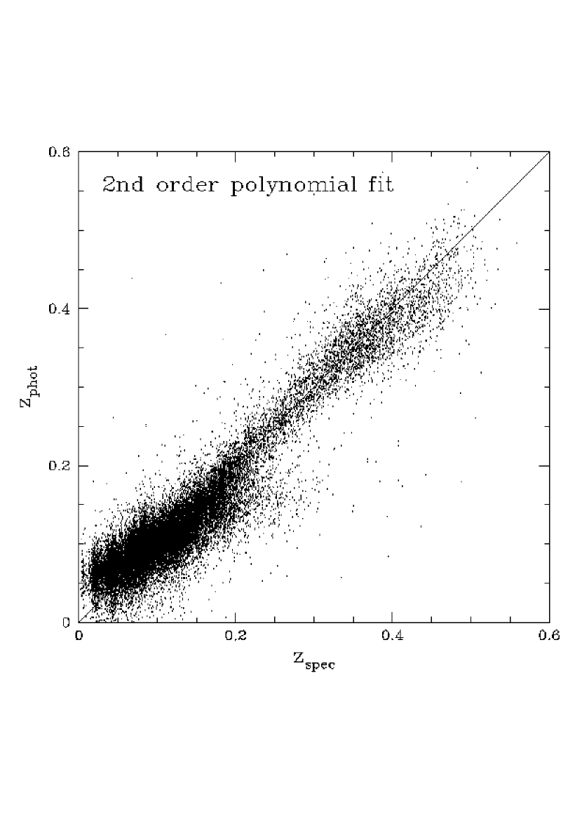
We consider here the standard empirical redshift estimation techniques that have been used in the literature (Connolly et al. (1995); Wang, Bahcall & Turner (1998); Brunner, Connolly & Szalay (1999)) and develop a new technique based on a hierarchical indexing structures (kd-trees,Moore (1995)). One of the first successful empirical methods is based on fitting a functional form for the relation between the spectroscopic redshift of a galaxy and its colors or magnitudes (Connolly et al. (1995)). This function is typically a 2nd or 3rd order polynomial. Figure 2 shows the photometric vs. the spectroscopic redshifts using the EDR main galaxy and LRG spectroscopic samples. As the size of the training set is large () when compared to the number of the fitted parameters (), we can expect that this fit will work for other objects with the same dispersion as seen in Figure 2 (as long as the data are selected over the sample color and redshift range as the training set). The dispersion within this photometric redshift relation is (see Table 1 for comparision with other values). One possible uncertainty within this technique comes from the fact that the fitting function is just an approximation of the, possibly, more complex relation between the colors and the redshift of a galaxy. We would, therefore, expect the fitting function to accurately follow the redshift-color relation over a narrow range of redshift. A technique to avoid this, is to use separate functions in different redshift (Brunner, Connolly & Szalay (1999)) or color ranges.
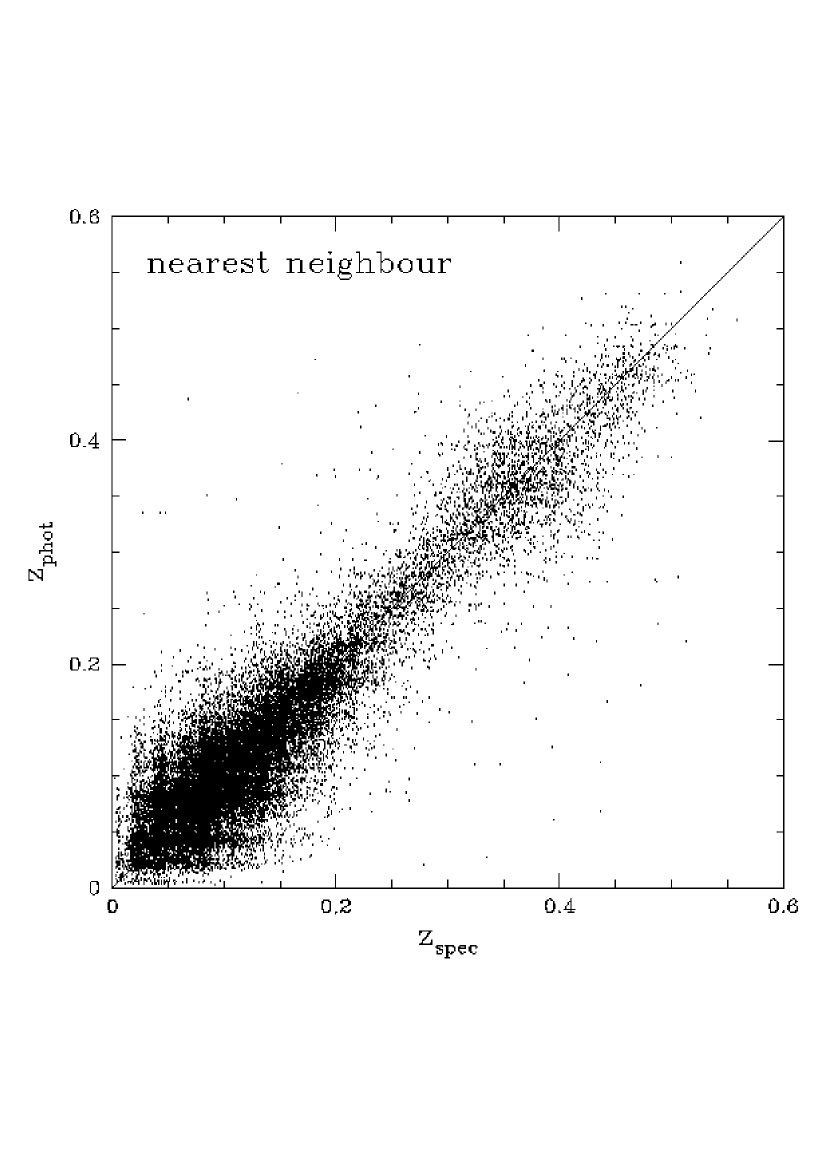
A second, and possibly the simplest, empirical estimator is the nearest neighbor method. For a test galaxy, this finds the galaxy within the training set with the smallest distance in the color (or magnitude) space (weighted by the errors). The redshift of this closest match is then assigned to the test galaxy. In the ideal case the training set contains sufficient galaxies that for each unknown object there is a close neighbor. In Figure 3 we show, that redshift estimation error increases with the distance from the nearest neighbor in color space. The larger the dataset the more accurate this method becomes, as long as that all galaxy types are represented in the training set. From the technical viewpoint, larger training sets mean that the search time increases so one has to use an efficient multidimensional search technique (e.g. kd-trees) instead of a standard linear search. The comparison between the estimated and spectroscopic redshifts for the nearest-neighbor technique is given in Figure 2. The dispersion about this relation is .
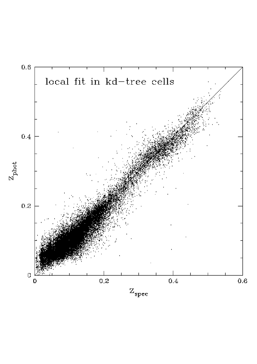
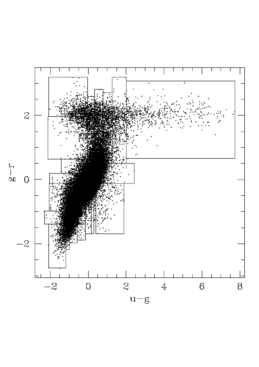
A natural limitation of the nearest neighbor technique is that a large number of training galaxies alone is not enough, they must cover the range of the colors of the unknown objects in a more or less uniform way. Unfortunately, this is usually not the case. To resolve this problem one can search for more than one nearest neighbor and apply an interpolation or a fitting function. This also helps to resolve a second problem, namely that because of the finite number of objects in the training set, the photometric redshifts will have discrete values making them problematic to use in some statistical studies. We have created a hybrid version of the above two empirical methods: we partitioned the color space into cells, containing the same number of objects from the training set, using a kd-tree tree (a binary search tree (Bentley, 1979)). In each cell we fit a second order polynomial. The results together with a demonstration of a 2-dimensional version of the kd-tree partitioning of the EDR training set are given in Figure 4. The dispersion about this relation is .
For each of these approaches the resulting dispersion in the photometric redshift relation is found to be approximately 0.03 (see Table 1 with the hybrid method being marginally more accurate. As these empirical approaches do not rely on the absolute photometric calibration of the data (other than the calibration should be stable across the data sets) they are somewhat insensitive to systematic errors in the data. If the SDSS redshifts (or external redshift samples) sampled the full redshift range of the data to the limit of the survey these empirical techniques would provide an ideal mechanism for deriving redshift estimates for the SDSS. As the redshift range of the spectroscopic samples are fairly limited the application of these techniques to the full data set is non-trivial. We can, however, use these results to demonstrate that accuracy we should be able to derive from the template based techniques (once any systematics within the data are accounted for) should be at .
3.2 Template Based Redshift Estimation Methods
As noted previously, the advantage of using templates to estimate redshifts of galaxies (Koo (1985); Gwyn & Hartwick (1996); Sawicki, Lin & Yee (1997); Connolly et al. (1999); Fernández-Soto et al. (1999); Benítez (2000); Bolzonella, Miralles & Pelló (2000); Budavári et al. (1999, 2000); Csabai et al. (2000)) are numerous. This approach simply compares the expected colors of a galaxy (derived from template spectral energy distributions) with those observed for an individual galaxy. The standard scenario for template fitting is to take a small number of spectral templates (e.g. E, Sbc, Scd and Irr galaxies) and choose the best fit by optimizing the likelihood of the fit as a function of redshift, type and luminosity . Variations on this approach have been developed in the last few decades including ones that use a continuous distribution of spectral templates enabling the error function in redshift and type to be well defined.
A representative set of spectrophotometrically calibrated spectral templates is not easy to obtain. One problem with measured spectra is, that to calibrate them spectrophotometrically over the full spectral range is non-trivial. A second problem is that, because of the redshift of a galaxy, we need spectra over a wavelength range that is wider than the range of our optical filters (3000–12000Å). Such spectra cannot currently be measured by a single spectrograph. Third, even if we could measure calibrated spectra over the required range, spectrographs, especially modern multifiber ones, usually sample only the central region of the galaxy while photometric measurements integrate over the full spatial extent of a galaxy. The alternative to empirical templates is to use the outputs of spectral synthesis models. The accuracy of spectral models are improving (Bruzual & Charlot, 1993) but not yet as accurate as direct measurements of galaxy spectra. Modern surveys will improve on this situation, e.g. the SDSS will measure spectrophotometrically calibrated spectra for a million objects in the 3800–9200Å range at a resolution of about 1800, but to-date there does not exist an optimal set of galaxy spectral templates.
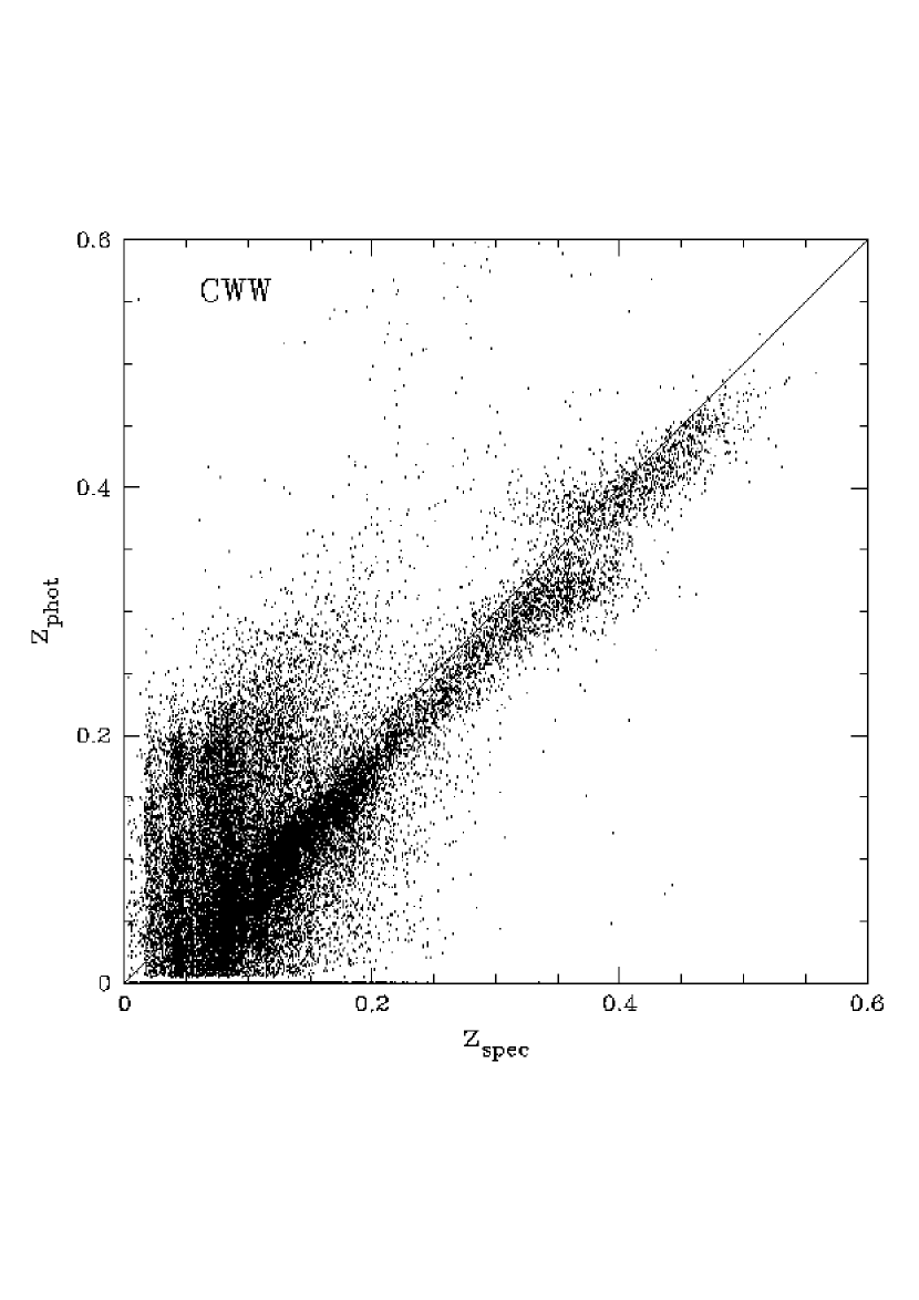
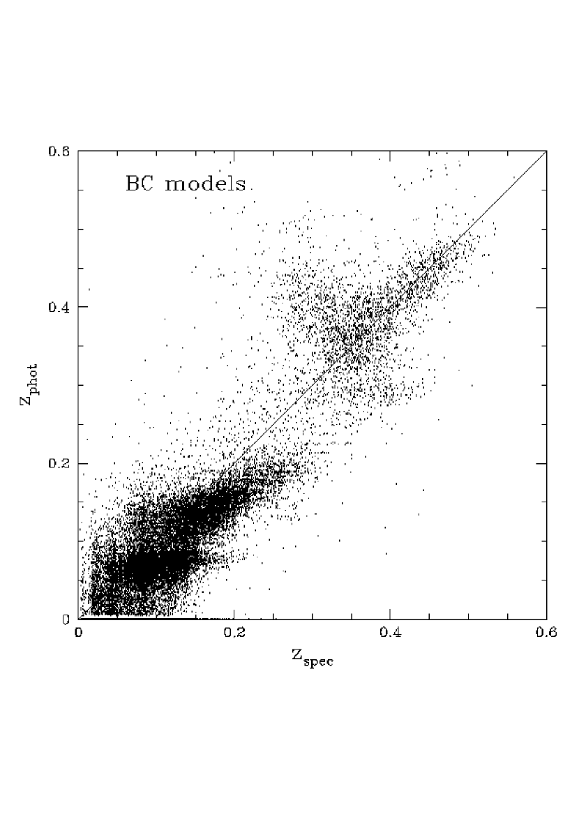
The most frequently used set of spectral energy distributions (SEDs) used in photometric redshift analyses are those from Coleman, Wu & Weedman (1980, hereafter CWW) (see also Bolzonella, Miralles & Pelló (2000)). In Figures 5 and 6 we demonstrate the results of the template fitting technique using the CWW templates and a set of SEDs from the spectral synthesis models of Bruzual & Charlot (1993). The dispersion about this relation is 0.062 and 0.051 for the CWW and BC templates respectively. While this is only a factor of two worse than that achieved by the empirical methods there appear to be systematic deviations within these photometric redshift relations. The CWW templates produce a photometric redshift relation where the majority of galaxies have a systematically lower redshift than that given by the spectroscopic data (by approximately 0.03 in redshift) and there exists a broad tail of galaxies for which the photometric redshifts are systematically overestimated. For the BC templates the galaxy redshifts tend to be systematically underestimated (with this effect becoming more pronounced as a function of redshift out to redshifts z=0.3).
An improvement over standard template methods, which rely uniquely on the galaxy colors, is the introduction of magnitude priors within a Bayesian framework (Benítez (2000)). The redshift distribution of the main EDR sample is well fitted by the relationship for , and a continuous prior can be constructed by we measuring in 5 different magnitude bins and interpolating. Since the EDR spectroscopic sample redshift distribution is ’contaminated’ by LRGs at faint magnitudes and turns bimodal, we have assumed a flat redshift/magnitude prior for . Using this magnitude prior we run Bayesian estimation, with two further refinements: a) setting the minimal photometric error in each band to 0.03, which mimics the intrinsic fluctuations in the colors of galaxies described by a same template and produces more realistic redshift likelihoods and b) using linear interpolation between the main CWW types to improve the color resolution. Using this setup, the dispersion for the CWW templates without using any prior decreases from 0.06 to 0.05, with an offset of 0.0156; introducing the prior described above further decreases the dispersion to (see Figure 7) for the whole sample, but an offset of 0.0144 still remains.
It is clear from these tests that while the template fitting methods should be directly applicable to the SDSS EDR data there remain significant systematics within either the templates or the photometric calibrations (or both) that will add artifacts into any photometric redshift relation. We must, therefore, recalibrate the template spectra to minimize these systematic effects.
4 Hybrid Photometric Redshift Techniques
Recently new hybrid techniques have been developed to calibrate template spectral energy distributions (SEDs) Csabai et al. (2000); Budavári et al. (1999, 2000, 2001a) using a training set of photometric data with spectroscopic redshifts. These combine the advantages of the empirical methods and SED fitting by iteratively improving the the agreement between the photometric measurements and the spectral templates. The basic approach is to divide a set of galaxies into a small number of spectral classes (using the standard template based photometric redshifts) and then to adjust the template SEDs to match the mean colors of the galaxies within these spectral classes. By repeating this classification and repair procedure the template spectra converge towards the observed colors. In this paper we will not review the details of these techniques but direct the reader to Csabai et al. (2000); Budavári et al. (1999, 2000, 2001a) for a full description of the algorithms. As we shall show in the following sections the application of these techniques yields more reliable photometric redshifts for the SDSS EDR catalog than the standard template fitting.
4.1 A Single Template: The Luminous Red Galaxy Sample
In addition to providing a training set for redshift estimation within the SDSS data the LRG sample is extremely useful in identifying systematic uncertainties within the SDSS photometric system. The LRG galaxies have a strong continuum feature, namely the break at around 4000Å. Due to the depth of this feature, photometric redshifts are easily estimated for these galaxies. In addition, due to the high luminosity of these galaxies they can be observed, spectroscopically over a larger redshift range than the main galaxy sample. Systematics within the photometric data can, therefore, be identified as this spectral feature passes through the filters as a function of redshift. In fact, we can simply use a single SED for the LRG sample to test how we must optimize the template spectra to accurately represent the observed colors.
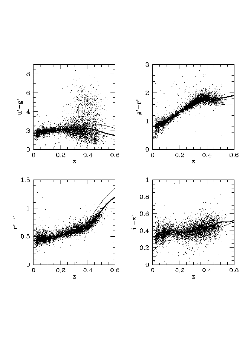
For the 6698 LRG galaxies we start with an initial template spectrum selected from the CWW elliptical spectrum and apply the training techniques of Budavari et al (2000). In Figure 8 we show the original CWW elliptical spectrum together with our reconstructed template. From these spectra we can see that in oder to represent the colors of the LRGs we need a template spectrum that is redder than the standard CWW elliptical. To demonstrate, how well these respective spectral templates cover the photometric observations, we have plotted, in Figure 9, the colors of the EDR LRG galaxies together with the traces of the original and repaired spectral templates. The color-redshift relation for the repaired spectrum clearly traces the locus of the LRG galaxy sample more accurately than the original CWW SED. The most obvious improvement in the comparative colors is found in the and colors.
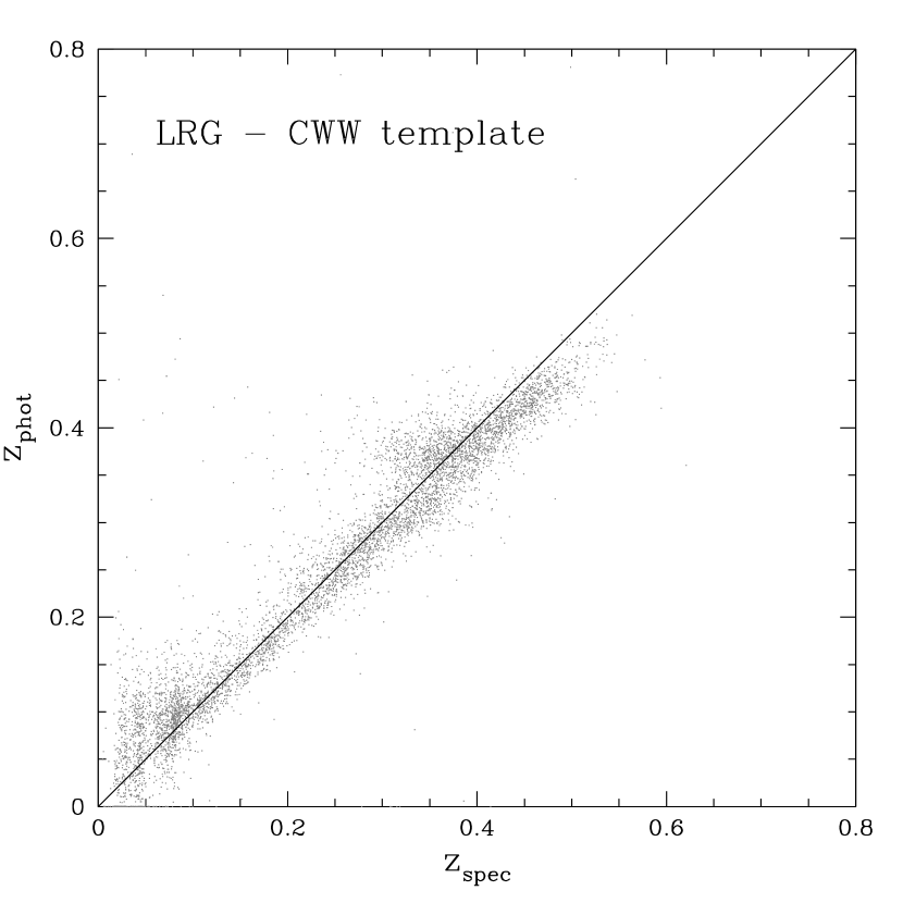
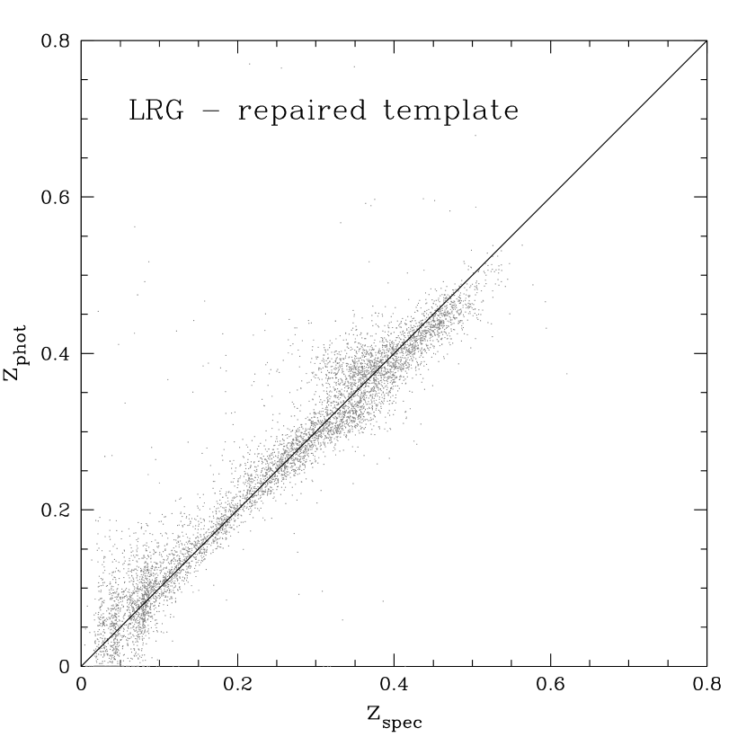
Although the repair procedure does not optimize directly for photometric redshifts, the improvement in the match between the observed and predicted colors should lead to an improved photometric redshift relation for the LRG sample. Figure 10 compares the performance of the photometric redshift estimators utilizing the two original and repaired template SEDs. The repair procedure decreases the overall scatter in the redshift relation from to . The main improvement is, however, that the systematic underestimation of the redshift, at redshifts , is reduced. There remains a feature in the redshift relation at , an increase, by a factor of two, in the dispersion. This arises due to the fact that there exists a degeneracy in the vs colors within red galaxies at a redshift of (the color-color tracks loop on top of each other). The degeneracy is a result of the Balmer break shifting between the and filters making it difficult to estimate the exact redshift (Budavári et al. (2001b)). This problem cannot be removed by using better template spectra.
4.2 The Distribution of Galaxy Types: The Main galaxy Sample
The entire sample of the SDSS galaxies (including the LRGs) poses a more difficult question due to the spectral composition of the data. Spectral variations cannot be neglected and, in fact, one would like to get a continuous parameterization of the spectral manifold. To accomplish this we adopt a variant of the ASQ algorithm (Budavári et al. (2001a)). First we reconstruct a small number of discrete SEDs using the techniques described previously and then we use an interpolation scheme to provide a continuous distribution of spectral types that evenly sample between the discrete spectra.
The training set consists of all galaxies with spectroscopic redshifts and the 5 band SDSS photometry. The large number of galaxies is very promising but the spectral resolution of the reconstructed templates also depends on the redshift baseline of the input galaxy training set. This redshift range is significantly smaller than, for example, those derived from the Hubble Deep Field (Hogg et al. (1998); Budavári et al. (2000)). Ideally, one would like to have a training set that uniformly samples the color space to ensure that no extra weight is assigned to any particular type of galaxy. The limited color range of the galaxies with spectroscopic redshifts will, therefore, ultimately limit the accuracy of our final redshift relations.
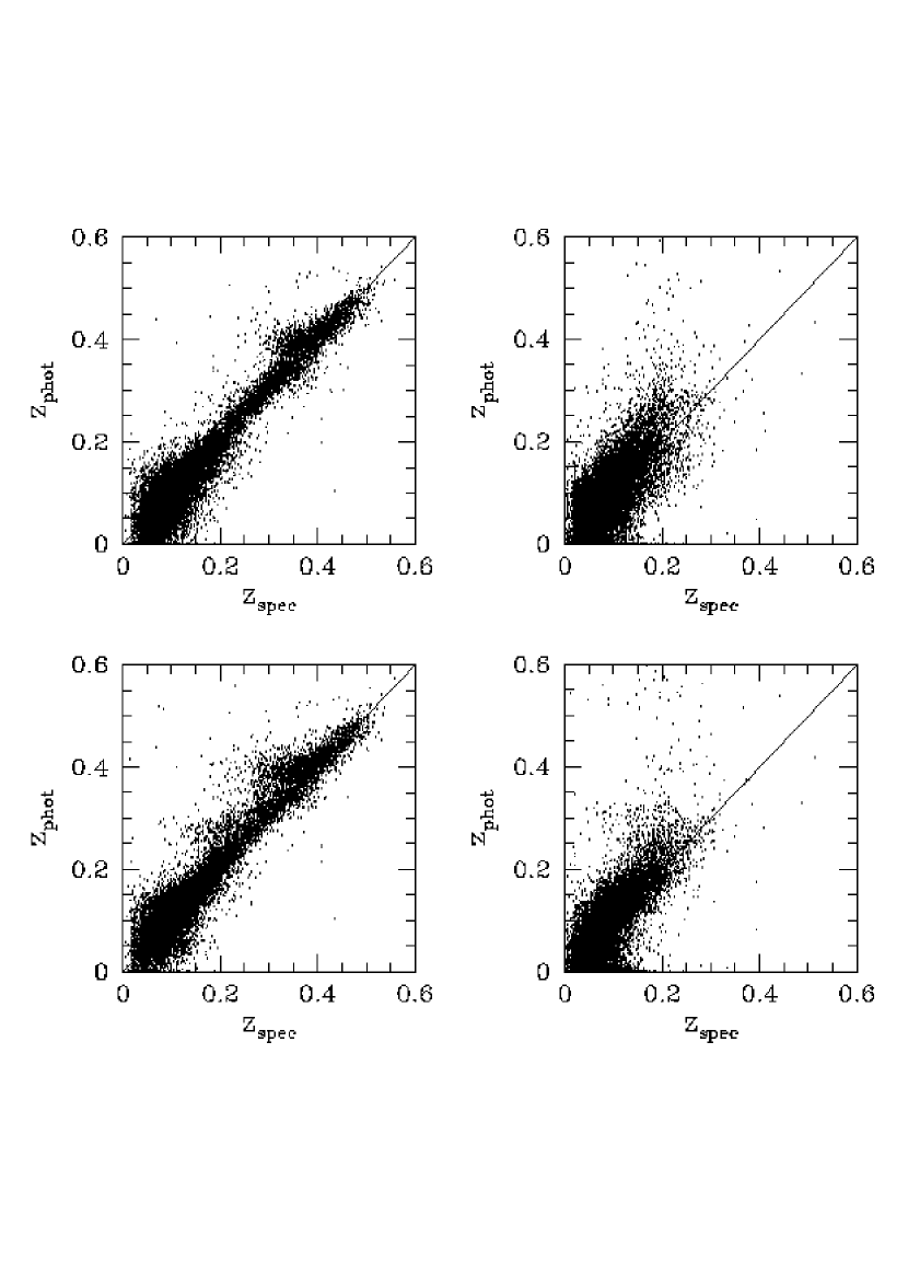
The iterative ASQ method was applied to the initial set of four CWW spectra. The spectral templates are found to converge rapidly, within a few iterations. After 10 iterations, the repaired templates yield photometric redshifts that are shown in the top panels of Figure 11. The left panel shows all galaxies assigned to the reddest template and the galaxies assigned to the remaining three templates are given on the right panel. The rms in the red and blue sample are and , respectively. This plot should be compared with the redshift relations derived from the standard CWW templates as shown in Figure 5. The training of these templates removes both the systematics within the data and reduces the dispersion about the photometric-redshift relation.
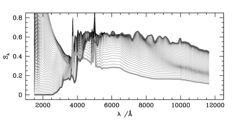
The large estimation error for the late type galaxies partly caused by the small number of discrete templates used in the redshift estimation. We can improve on our estimates if we derive an interpolation scheme that provides a finer sampling of the distribution of late type spectral templates. Figure 12 illustrates the 1D continuous spectral manifold derived from the discrete SEDs by plotting equally spaced (in type) interpolated spectra using a simple spline interpolation. Based on the following tests this simple interpolation scheme provides sufficient accuracy for mapping the color distribution of late type galaxies.
The first test of the interpolation scheme was a simple sanity check of the type histogram. If the interpolated spectra are not physical, we expect to see humps at the basis templates (i.e. the colors of the majority of galaxies will be better matched to the original templates than the interpolated templates). For this test, we used the known redshift of each galaxy in the training set and only fit the spectral type (and apparent luminosity). In Figure 13 we show this interpolated type histogram. The smooth transition between interpolated types shows no evidence for any discreteness in assigning a spectral template to an individual galaxy. The second test of the interpolation was to determine if the interpolated templates would evolve if we applied the ASQ training algorithm. Fixing the four basis trained SEDs, we introduced three interpolated classes at the center of the intervals between these spectral types. We find no significant change in the spectral properties of these interpolated spectra as a function of iteration of the training algorithm.
The redshift estimates based on the continuous 1D type parameter are shown in the bottom panels of Figure 11 for both the early- and late-type subsamples (left and right, respectively). Compared to the top panels of the discrete version (discussed previously), the new estimates seem to be superior for the intrinsically blue subset and slightly worse of the early-types.
For early-type galaxies it would be better to use the original discrete template set to avoid the systematic overestimation around and . Since we want to have a simple estimation for the spectral type, we would like to avoid to use a separate (discrete) template set for early-type galaxies, so we use the above scheme keeping in mind the systematic errors, and working on a better interpolated template set. Note, that SDSS will measure spectroscopic redshift for most of the luminous early-type galaxies, so the number of objects where this problem arises is somewhat smaller than in our test sample. Though for the less luminous early type galaxies the above problem still exist.
In terms of rms values of the scatter this translates to an increase from to for the red galaxies and a decrease from to for the blue ones. To quote an rms for the entire training set would not be to meaningful because it depends on the ratio of the number of early- and late-type galaxies. For the main SDSS galaxy sample the scatter is . We will use the above template fitting method with repaired interpolated templates to create the EDR photometric redshift catalog.
5 Comparisons with Independent Redshift Samples
5.1 The 2dF and CNOC2 Redshift Samples
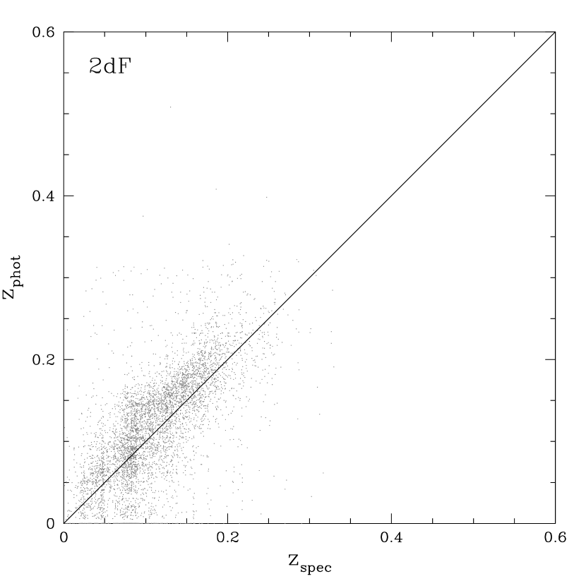
In the above sections we have used data from the same subsets for training and testing. We now perform a blind test using the independent data sets. Details of the 2dF and CNOC2 data sets are given in Section 2. Figure 14a compares the spectroscopic and photometric redshifts for the 2dF spectroscopic sample. The dispersion within the photometric-redshift relation for these data is, . This compares to the dispersion in the relation for the full SDSS sample of . The increase in the dispersion arises from two effects. The band magnitudes of the 2dF data are intrinsically fainter than the SDSS spectroscopic sample (by approximately 0.2 magnitudes) and the 2dF data are selected based on their photographic magnitudes which will provide an intrinsically bluer galaxy sample than the selected SDSS data. As the dispersion in the redshift relation increases with limiting magnitude and for blue galaxies the difference in the observed photometric redshift relation is not surprising.
To determine how well the templates extrapolate to higher redshift data we apply the photometric redshifts to the CNOC2 data set (with a redshift range and a magnitude limit of ) As we can see in Figure 14 the dispersion in the relation increases for the fainter magnitude sample due to the increase in photometric error. The average estimation error for the whole set is . If we consider only those galaxies with , the uncertainty in the redshift estimates decreases to . In Figure 15 we show the absolute deviation between the photometric and spectroscopic redshifts for the CNOC2 galaxy sample as a function of . The cumulative rms of these data (as a function of ) is shown by the solid line. For the rms uncertainty about this relation is 0.1 in redshift.
6 The Early Data Release Photometric Redshift Catalog
6.1 Selecting Galaxies From the EDR Database
The goal of our analysis has been to obtain photometric redshifts for all SDSS galaxies in the Early Data Release. We have, therefore, created the first EDR photo-z catalog (version 1.0) which has now been included in the publicly available EDR database at http://skyserver.sdss.org/.
We used the template fitting method with repaired interpolated templates 4 to estimate photometric redshifts in the above public catalog. Though the empirical methods (see 3.1) give smaller estimation error, we have chosen to use the template fitting method since it estimates not just redshift, but spectral type and restframe magnitude, too. Also we hope, that with the accumulation of more precisely calibrated data in further SDSS releases, the disadvantage of this method decreases.
The photometric redshift table (see Table 2 for the list of parameters) in the database has more than 6 million entries, one for every galaxy in the EDR. Each entry contains the unique object ID (objID, for quick cross-matching), the most likely redshift (z) and type (t). The uncertainties of redshift and type calculated from the 68% confidence regions of the fit assuming Gaussian errors. Note that the true error distribution for higher redshift object is not known, and probably not Gaussian. The elements of the covariance matrix are stored in the database and represented by c_zz, c_tt, c_tz. The errors in columns zErr and tErr are simply taken from the diagonal elements of the covariance matrix. The value of the fit (chiSq) measures the absolute ‘goodness’ of the fit. The catalog contains a preliminary quality flag (quality), which scales between zero and five where the larger the number the more confident the photometric redshift. This flag is assigned to objects in the process of fitting the confidence region and seems to correlate with the rms of the photometric and spectroscopic redshifts. In the current version this correlation is quite weak, we would like to improve the calculation of this flag in the next version.
In addition to the redshift estimates physical parameters derived from the estimated redshift are also stored within the database. These include the distance modulus (dmod) for the standard CDM cosmology (, , units), restframe colors (rest_ug, rest_gr, rest_ri, rest_iz) and K-corrections (kcorr_u, kcorr_g, kcorr_r, kcorr_i, kcorr_z) derived directly from the templates and the restframe absolute magnitudes (absMag_u, absMag_g, absMag_r, absMag_i, absMag_z) as computed from the distance modulus and K-correction,
Access to these parameters is straightforward through the Structured Query Language (a.k.a. SQL). A sample query to extract the objId and photometric redshift of 5 galaxies in the redshift range of would look like this:
select top 5 objId, z from PhotoZ where z>0.2 and z<0.3
All parameters stored within the SDSS database (including the derived parameters) can be searched upon.
6.2 Caveats and Limitations of the Current Photometric Redshifts
While, as the comparisons between the photometric and spectroscopic redshift show, the current implementation of SDSS photometric redshifts provide an accurate estimate of the redshifts there are a number of limitations and caveats pertaining to the EDR data. We describe here the results of a series of tests of the quality of the SDSS photometry and how these issues affect the accuracy and possible uses of the photometric redshifts in the EDR catalog. We advise any potential user of the current photometric redshift implementation to be aware of these caveats prior to undertaking any statistical analysis.
Even though the photometric calibration of the SDSS survey has been shown to be be accurate to a few percent for the SDSS standard stars, galaxy colors appear to have a slight offset from SED based estimated values (Eisenstein et al. (2001)). As part of this analysis of the SDSS EDR data we compare measured colors not only to the spectrophotometrically calibrated SEDs (e.g. CWW) but we have also carried out experiments where small offsets were applied before the refining the template spectra. In this way we can identify systematic photometric offsets from the mean deviation of the colors from the SEDs. The band offset we found is in the same sense as that given in Eisenstein et al. (2001) but with a smaller amplitude of . All galaxies within the SDSS catalog had this offset applied prior to calculation of the photometric redshifts.
Our SED reconstruction algorithm ideally requires a training set with reasonably uniform redshift distribution over a large baseline. The SDSS spectroscopic survey delivers excellent quality data for this kind of analyses. However, the main galaxy sample has a median redshift of approximately 0.1 which does not enable the use photometric data from different bands to constrain the SEDs at all wavelengths. In principle, if there exist photometric zeropoint uncertainties within the data, the reconstruction could introduce artificial continuum spectral features in the templates that would make the extrapolation to higher redshifts impossible (in a similar sense to the limitations of the empirical techniques). The repaired spectral energy distributions show no obvious trace of such features.
Finally, we consider how the increasing photometric uncertainty at fainter magnitudes affect the redshift histograms. In Figure 16 we show the redshift distributions in different magnitude bins 16–17, 17–18, 18–19, 19–20 and 20–21. The histograms built in different magnitude bins peak around values consistent with published redshifts surveys and that move toward higher values as a function of the magnitude. Beyond a magnitude limit of artifacts are seen within the redshift histograms due to the large photometric errors. We, therefore, advise caution when using the current EDR photometric redshift catalog for galaxies with . Also one should take into consideration the fact that for some objects the photometric redshift would be negative because the estimation is based on photometric data with errors, but the algorithm allows only positive redshift values, so all negative redshifts pile up at .
7 Conclusions
We present the first application of photometric redshifts to the SDSS EDR data. From a comparison of the photometric and spectroscopic redshifts we find that the rms error within the redshift relation is for rising to 0.1 at . For magnitude intervals the photometric redshift relation and redshift histogram are well matched to existing redshift surveys (with comparable median redshifts and dispersions). Implementing these redshift estimates in the SDSS EDR database, together with derived quantities such as the absolute magnitudes, k-corrections and restframe colors, we provide a simple interface to one of the largest publicly accessible catalogs of photometric redshifts available to the astronomical community. We conclude by providing a description of the limitations and caveats present within the current photometric redshift implementation. We caution all users to be aware of these limitations before applying the EDR photometric redshifts in any statistical analyses.
References
- Benítez (2000) Benítez, N., 2000, ApJ, 536, 571
- Bentley (1979) J. L. Bentley, 1979, Communications of the ACM 19, 509
- Bolzonella, Miralles & Pelló (2000) M. Bolzonella, J.-M. Miralles, R. Pelló, 2000, A&A, 363, 476
- Brunner, Connolly & Szalay (1999) Brunner, R.J., Connolly, A.J., & Szalay, A.S., 1999, ApJ, 516, 563
- Bruzual & Charlot (1993) Bruzual, A.G., & Charlot, S., 1993, ApJ, 405, 538
- Budavári et al. (1999) Budavári, T., Szalay, A.S., Connolly, A.J., Csabai, I., & Dickinson, M.E., 1999, in Photometric Redshifts and High Redshift Galaxies, eds. R.J. Weymann, L.J. Storrie–Lombardi, M. Sawicki, & R. Brunner, (San Francisco: ASP), 19
- Budavári et al. (2000) Budavári, T., Szalay, A.S., Connolly, A.J., Csabai, I., & Dickinson, M.E., 2000, AJ, 120, 1588
- Budavári et al. (2001a) Budavári, T. et al., 2001, AJ, 122, 1163
- Budavári et al. (2001b) Budavári, T. et al., 2001, AJ, 121, 3266
- Coleman, Wu & Weedman (1980) Coleman, G.D., Wu., C.-C., & Weedman, D.W., 1980, ApJS, 43, 393
- Colless et al. (2001) Colless M.M et al., 2001, MNRAS, 328, 1039
- Connolly et al. (1995) Connolly, A.J., Csabai, I., Szalay, A.S., Koo, D.C., Kron, R.G., & Munn, J.A., 1995, AJ, 110, 2655
- Connolly et al. (1999) Connolly, A.J., Budavári, T., Szalay, A.S., Csabai, I., & Brunner, R.J., 1999, in Photometric Redshifts and High Redshift Galaxies, eds. R.J. Weymann, L.J. Storrie–Lombardi, M. Sawicki, & R. Brunner, (San Francisco: ASP), 13
- Csabai et al. (2000) Csabai, I., Connolly, A.J., Szalay, A.S., & Budavári, T., 2000, AJ, 119, 69
- Eisenstein et al. (2001) Eisenstein D.J. et al., 2001, AJ, 122, 2267
- Fernández-Soto et al. (1999) Fernández-Soto, A., Lanzetta, K.M., & Yahil, A., 1999, ApJ, 513, 34
- Fukugita et al. (1996) Fukugita, M., Ichikawa, T., Gunn, J.E., Doi, M., Shimasaku, K. & Schneider, D.P. 1996, AJ, 111, 1748
- Gunn et al. (1998) Gunn, J.E., Carr, M.A., Rockosi, C.M., Sekiguchi, M., et al. 1998, AJ, 116, 3040
- Gwyn & Hartwick (1996) Gwyn, S.D.J., & Hartwick, F.D.A., 1996, ApJ, 468, L77
- Hogg et al. (1998) Hogg, D.W, et al., 1998, ApJ, 499, 555
- Hogg et al. (2001) Hogg, D.W., Schlegel, D.J., Finkbeiner, D.P., & Gunn, J.E. 2001, AJ, 122, 2129
- Koo (1985) Koo, D.C., 1985, AJ, 90, 148
- Madau (1995) Madau, P., 1995, ApJ, 441, 18
- Moore (1995) Moore, A.W., Schneider, J. & Deng, K., 1997, Proceedings of the 1997 International Machine Learning Conference, eds Fisher D., Morgan Kaufmann
- NASA/IPAC Extragalactic Database (NED) http://nedwww.ipac.caltech.edu/
- Sawicki, Lin & Yee (1997) Sawicki, M.J., Lin, H., & Yee, H.K.C, 1997, AJ, 113, 1
- Smith et al. (2002) Smith, J.A., Tucker, D.L., Kent, S.M., et al. 2002, AJ, 123, 2121
- Stoughton et al. (2002) Stoughton C. et al., 2002, AJ, accepted
- Strauss et al. (2002) Strauss M.A. et al., 2002, in preparation
- Pier et al. (2002) Pier, J.R., Munn, J.A., Hindsley, R.B., Hennessy, G.S., Kent, S.M., Lupton, R.H., & Ivezic, Z. 2002, AJ, submitted
- Yee et al. (1996) Yee et al., 1996, ApJS, 102, 269
- SDSS; York et al. (2000) York, D.G., et al., 2000, AJ, 120, 1579
- Wang, Bahcall & Turner (1998) Wang, Y., Bahcall, N., & Turner, E.L., 1998, AJ, 116, 2081
- Williams et al. (1996) Williams, R.E., et al., 1996, AJ, 112, 1335







| Estimation Method | rms | log | iterated | non-outliers | |
|---|---|---|---|---|---|
| Polynomial | 0.0318 | 0.0277 | 0.0273 | 98.0% | |
| Nearest neighbor | 0.0365 | 0.0321 | 0.0327 | 98.5% | |
| Kd-tree | 0.0254 | 0.0224 | 0.0226 | 98.4% | |
| CWW | 0.0666 | 0.0598 | 0.0621 | 99.1% | |
| Bruzual-Charlot | 0.0552 | 0.0501 | 0.0509 | 99.2% | |
| Bayesian | 0.0476 | 0.0415 | 0.0422 | 98.4% | |
| CWW LRG | 0.0473 | 0.0332 | 0.0306 | 97.1% | |
| Repaired LRG | 0.0476 | 0.0319 | 0.0289 | 96.5% | |
| Interpolated | 0.0451 | 0.0359 | 0.0352 | 97.7% | |
| 2dF | 0.0528 | 0.0455 | 0.0433 | 97.1% | |
| CNOC2 | 0.1358 | 0.0989 | 0.0842 | 93.0% | |
| CNOC2 | 0.0801 | 0.0614 | 0.0614 | 97.1% |
Note. — We list 3 different estimated rms values in the Table. The first is the usual standard deviation computed for all galaxies as defined by , where . The standard deviation is very sensitive to outliers, it is a common trick to assign less weight to them by defining another quantity that measures the scatter in a more reliable way: where is a large number compared to . We use , where is the median. Without outliers and were basically same, because for small values, but large outliers only affect the standard deviation drammatically. Another way of suppressing the effect of outliers is excluding them. The last rms column (; we use this values in the text) lists the standard deviation for galaxies that are within the limits of the distribution, which often has a value similar to . The very last column of the table shows the fraction of galaxies included in the limit.
| name | type | length | unit | description | |
|---|---|---|---|---|---|
| int | 4 | - | unique Id for photoz version | ||
| int | 4 | - | the rank of the photoz determination, default is 0 | ||
| varchar | 6 | - | the version of photoz code | ||
| int | 4 | - | char describing the object type (galaxy:1, QSO:tbd, …) | ||
| bigint | 8 | - | unique ID pointing to PhotoObj table | ||
| real | 4 | - | the chi-square value for the fit | ||
| real | 4 | - | photometric redshift | ||
| real | 4 | - | the marginalized error of the photometric redshift | ||
| real | 4 | - | photometric SED type between 0 and 1 | ||
| real | 4 | - | the marginalized error of the photometric type | ||
| real | 4 | - | tt element of covariance matrix | ||
| real | 4 | - | tz element of covariance matrix | ||
| real | 4 | - | zz element of covariance matrix | ||
| int | 4 | pixels | radius of area used for covariance fit | ||
| real | 4 | - | probability threshold for fitting, peak normalized to 1 | ||
| int | 4 | - | integer describing the quality (best:5, lowest 0) | ||
| real | 4 | magnitudes | distance modulus for Omega=0.3, Lambda=0.7 cosmology | ||
| real | 4 | magnitudes | rest frame u-g color | ||
| real | 4 | magnitudes | rest frame g-r color | ||
| real | 4 | magnitudes | rest frame r-i color | ||
| real | 4 | magnitudes | rest frame i-z color | ||
| real | 4 | magnitudes | k correction | ||
| real | 4 | magnitudes | k correction | ||
| real | 4 | magnitudes | k correction | ||
| real | 4 | magnitudes | k correction | ||
| real | 4 | magnitudes | k correction | ||
| real | 4 | magnitudes | rest frame u’ abs magnitude | ||
| real | 4 | magnitudes | rest frame g’ abs magnitude | ||
| real | 4 | magnitudes | rest frame r’ abs magnitude | ||
| real | 4 | magnitudes | rest frame i’ abs magnitude | ||
| real | 4 | magnitudes | rest frame z’ abs magnitude |
Note. — The parameters contained in the Table of the SDSS Science Archive http://skyserver.sdss.org/. See text for more details.