Spin Induced Galaxy Alignments and their implications for weak lensing measurements

Abstract

Large scale correlations in the orientations of galaxies can result from alignments in their angular momentum vectors. These alignments arise from the tidal torques exerted on neighboring proto-galaxies by the smoothly varying shear field. We compute the predicted amplitude of such ellipticity correlations using the Zel’dovich approximation for a realistic distribution of galaxy shapes. Weak gravitational lensing can also induce ellipticity correlations since the images of neighboring galaxies will be distorted coherently. On comparing these two effects that induce shape correlations, we find that for current weak lensing surveys with a median redshift of $z_{m}=1$, the intrinsic signal is of order 1-10% of the measured signal. However, for shallower surveys with $z_{m}\leq 0.3$, the intrinsic correlations dominate over the lensing signal. The distortions induced by lensing are curl-free, whereas those resulting from intrinsic alignments are not. This difference can be used to disentangle these two sources of ellipticity correlations.

1 Department of Applied Mathematics and Theoretical Physics, Wilberforce Road, Cambridge CB3 0WA, UK

2 Institute of Astronomy, Madingley Road, Cambridge CB3 0HE, UK

3 Department of Astronomy, Yale University, New Haven, CT, USA

4 CITA, McLennan Labs, University of Toronto, Toronto, M5S 3H8

Draft version

1 Introduction

Gravitational lensing can be used to map the detailed distribution of matter in the Universe over a range of scales (Gunn 1967). Systematic distortions in the shapes and orientations of high redshift background galaxies are induced by mass inhomogeneities along the line of sight. In strong lensing, a single massive foreground cluster will cause background galaxies to be significantly magnified and distorted. Weak lensing, on the other hand, measures the cumulative effect of less massive systems along the line of sight statistically (Gunn 1967; Blandford et al. 1991; Miralda-Escude 1991; Kaiser 1992; see a recent review by Bartelmann & Schneider 1999).

The lensing effect depends only on the projected surface mass density and is independent of the luminosity or the dynamical state of the mass distribution. Thus, this technique can potentially provide invaluable constraints on the distribution of matter in the Universe and the underlying cosmological model (Bernardeau, van Waerbeke & Mellier 1997; van Waerbeke, Bernardeau & Mellier 1999). There has been considerable progress in theoretical calculations of the effects of weak lensing by large-scale structure, both analytically and using ray-tracing through cosmological N-body simulations (Kaiser 1992; Bernardeau, van Waerbeke & Mellier 1997; Jain & Seljak 1997; Jain, Seljak & White 2000).

Recently, several teams have reported observational detections of ‘cosmic shear’ – weak lensing on scales ranging from an arc-minute to ten arc-minutes (Van Waerbeke et al. 2000; Bacon, Refregier & Ellis 2000; Wittman et al. 2000; Kaiser, Wilson & Luppino 2000). At present, these studies are limited by observational effects, such as shot noise due to the finite number of galaxies and the accuracy with which shapes can actually be measured given the optics and seeing (Kaiser 1995; Bartelmann & Schneider 1999; Kuijken 1999). In addition, the intrinsic ellipticity distribution of galaxies and their redshift distribution is still somewhat uncertain. These observational difficulties can be potentially overcome with more data.

However, an important theoretical issue remains. In modeling the distortion produced by lensing, it is assumed that the a priori intrinsic correlations in the shapes and orientations of background galaxies are negligible. Correlations in the intrinsic ellipticities of neighboring galaxies are expected to arise from the galaxy formation process, for example as a consequence of correlations between the angular momenta of galaxies when they assemble. We compute the strength of these correlations in linear theory, in the context of Gaussian initial fluctuations.

To do so, we approximate the projected shape of a galaxy on the sky by an ellipsoid with semi-axes $a$, $b$ ($a>b$). The orientation of the ellipsoid depends on the angle $\psi$ between the major axis and the chosen coordinate system, while its magnitude is given by $|\epsilon|=(a^{2}-b^{2})/(a^{2}+b^{2})$. Both the magnitude of the ellipticity and its orientation can be concisely described by the complex quantity $\epsilon^{(o)}$,

$$\epsilon^{(o)}=|\epsilon^{(o)}|e^{2i\psi}=[\epsilon_{+}^{(o)}+i\epsilon_{\times}^{(o)}].$$ (1)

where the superscript ^(o) denotes the observed shape.

In the linear regime and under the assumption of weak lensing, the lensing equation can be written as,

$$\epsilon^{(o)}\,=\,\frac{\epsilon\,+\,g}{1\,+\,g^{*}\epsilon},$$ (2)

where $g$ is the complex shear and $\epsilon$ the intrinsic shape of the source (Kochanek 1990; Miralda-Escude 1991). Furthermore, in the weak regime, correlations of this distortion field are

$$\langle{\epsilon^{(o)}}(\mathbf{x_{1}})\,{\epsilon^{(o)*}}(\mathbf{x_{2}})\rangle\,\simeq\,\langle{\epsilon(\mathbf{x_{1}})}\,{\epsilon^{*}}(\mathbf{x_{2}})\rangle\,+\,\langle{g^{*}}(\mathbf{x_{2}}){\epsilon(\mathbf{x_{1}})}+{g(\mathbf{x_{1}})}{\epsilon^{*}}(\mathbf{x_{2}})\rangle\,+\,\langle{g(\mathbf{x_{1}})}{g^{*}}(\mathbf{x_{2}})\rangle\,$$ (3)

where the ^∗ denotes complex conjugation. In this paper we will examine the first term, which arises from intrinsic shape correlations. Previous analyses have focused on the third term of this expression, correlations due to weak lensing. The second term, which is due to correlations between the lensing galaxies and the intrinsic shapes of the galaxies being lensed, will not be addressed here. Naively however, we expect this contribution to be small, since the mean distance between the lensing and lensed galaxies far exceeds the distance scale over which angular momentum correlations are important.

We will assume that shape correlations arise primarily from correlations in the direction of the angular momentum vectors of neighboring galaxies. Spiral galaxies are disk-like with the angular momentum vector perpendicular to the plane of the disk, so that angular momentum couplings will be translated into shape correlations. We will assume that for ellipticals the angular momentum vector also lies along its shortest axis on average, as it does for the spirals. However, since elliptical galaxies are intrinsically more round, the correlation amplitude will be smaller. Below we will use the observed ellipticity distributions of each morphological type in the computation of the shape correlations. For weak lensing, in contrast, the induced shape correlations are independent of the original shapes of the lensed galaxies. In the next sub-sections we will briefly review the origin of angular momentum and recent work on understanding intrinsic ellipticity correlations.

1.1 Origins of Angular Momentum

The angular momentum of the matter contained in a volume $V$ is defined as,

$${\mathbf{L}}(t)=\int_{V}[{\mathbf{r}}(t)-{\bar{\mathbf{r}}}(t)]\times{\mathbf{v}}({\mathbf{r}},t)\,\rho({\mathbf{r}},t)\,d^{3}r,$$ (4)

where ${\bar{\mathbf{r}}}$ is the center of mass and $\rho({\mathbf{r}},t)$ is the density. Hoyle (1949) suggested that the origin of galactic angular momentum is tidal torquing between the proto-galaxy and the surrounding matter distribution. Most of the angular momentum of an object is imparted before the over-dense region completely collapses. After collapse, tidal torquing will be inefficient and the object will simply conserve its spin.

Peebles (1969) used perturbation theory to calculate the growth rate of angular momentum contained within a comoving spherical region. For such a spherical region, there are no torques initially, so the growth occurs at second order as a result of convective effects on the bounding surface. In contrast, Doroshkevich (1970) showed that the angular momentum of a proto-galaxy grows at first order since, in general, proto-galactic regions are not spherical, generating an initial tidal torque. White (1984) described this process using the Zel’dovich (1970) approximation and showed that the spin grows linearly in time, for an Einstein-de Sitter universe.

Following White (1984), we consider the growth of fluctuations in an expanding Friedmann Universe filled with pressure-free dust ($p=0$) in Lagrangian perturbation theory. The trajectory of a dust particle can be written in comoving coordinates ${\mathbf{x}}={\mathbf{r}}/a$ in terms of the gradient of the gravitational potential $\Psi$, ${\mathbf{x}}({\mathbf{q}},t)={\mathbf{q}}-D(t)\nabla\Psi$ (Zeldovich 1970). $D(t)$ describes the growth of modes in linear theory and is proportional to the cosmological expansion factor, $a(t)$, for an Einstein de-Sitter model. In terms of the Lagrangian coordinates ${\mathbf{q}}$, the expression for angular momentum becomes

$${\mathbf{L}}(t)=\rho_{0}a^{5}\int_{V_{L}}[{\mathbf{x}}-{\bar{\mathbf{x}}}]\times{\mathbf{\dot{x}}}\,\,d^{3}q\simeq\rho_{0}a^{5}\int_{V_{L}}[{\mathbf{q}}-{\bar{\mathbf{q}}}]\times{\mathbf{\dot{x}}}\,\,d^{3}q,$$ (5)

where $\rho_{0}$ is the present mean matter density and $V_{L}$ is the Lagrangian volume that corresponds to $V$. The latter expression is correct to second order since ${\mathbf{\dot{x}}}=-\dot{D}(t)\nabla\Psi$ is parallel to the displacement.

We can progress by expanding the gradient of the gravitational potential in a Taylor series around the center of mass,

$$\partial_{\alpha}\Psi({\mathbf{q}})\simeq\partial_{\alpha}\Psi({\bar{\mathbf{q}}})+({\mathbf{q}}-{\bar{\mathbf{q}}})_{\beta}T_{\alpha\beta}$$ (6)

where the shear tensor is defined as the second derivative of the gravitational potential, $T_{\alpha\beta}({\mathbf{q}})\,=\,\partial_{\alpha}\,\partial_{\beta}\,\Psi({\mathbf{q}}).$ The angular momentum of a collapsing proto-galactic region before turnaround then is given by,

$$L_{\alpha}\,=\,a^{2}(t)\,{\dot{D}}(t)\,\epsilon_{\alpha\beta\gamma}\,T_{\beta\sigma}\,I_{\sigma\gamma},$$ (7)

$I_{\sigma\gamma}$ is the moment of inertia of the matter in the collapsing volume,

$$I_{\sigma\gamma}=\rho_{0}a^{3}(t)\int_{V_{L}}({\mathbf{q}}-{\bar{\mathbf{q}}})_{\sigma}({\mathbf{q}}-{\bar{\mathbf{q}}})_{\gamma}d^{3}q.$$ (8)

Note that the volume element that initially contains the matter is in fact much larger than that of the final galaxy in comoving coordinates. In this picture, the angular momentum is constant after turnaround.

This formalism has been used to study how angular momentum arises during galaxy formation. Heavens and Peacock (1988) used Eulerian perturbation theory to compute the modulus of the angular momentum for galaxies, assuming the object to form at the peak of a Gaussian field (Bardeen et al. 1986). They found that there is a broad distribution in the angular momenta of collapsed objects, which is only weakly correlated with the heights of the density peaks around which galaxies form.

Catelan & Theuns (1996a [CT96a]) expanded on this, working in Lagrangian space instead of Eulerian space. The results from these two approaches are very similar, but the resulting expressions are simpler for the Lagrangian case. CT96a approximated the shape of the object in Lagrangian space by an ellipsoid, which allowed the study of how angular momentum was correlated with other aspects of the matter distribution, such as its mass or its prolateness. The results of this analysis allows one to compute joint probability distributions, for example between the mass and spin of a halo. These were found to be in good agreement with the results from numerical simulations (Sugerman, Summers and Kamionkowski 2000).

Extending their approach, Catelan and Theuns (1996b) used second-order Lagrangian perturbation theory to estimate the contribution of non-linear effects, which they showed to be small. They also investigated the consequences of non-Gaussian primordial perturbations (Catelan & Theuns 1997), which they showed could have a significant effect on galactic spins.

Lee & Pen (2000) re-examined the origin of angular momentum on galaxy scales and studied the statistics of both the magnitude and the direction of the present day spin distribution using numerical simulations. They developed a method to reconstruct the gravitational field, using only the direction of the angular momenta, since the predictions for its magnitude have a large variance. A central issue in determining the magnitude of $L$ is the degree of correlation between the principal axes of the inertia tensor and gravitational shear tensor. CT96a attempted to take this into account around peaks, and found that such a correlation reduces the angular momentum by a small factor. Lee & Pen (2000) demonstrated using numerical simulations that this factor is in fact non-negligible. They however conclude that the approximation made by CT96a is adequate for determining the direction of the angular momentum vector but not for the magnitude. Here we extend the treatment of Lee & Pen (2000) and much of our notation and formalism follows their paper.

1.2 Intrinsic Ellipticity Correlations

There have been a number of preprints on this subject recently. We briefly review some of the results obtained by other groups here and we will compare our calculations and results with these in more detail in subsequent sections.

Two groups, Heavens et al. (2000) and Croft & Metzler (2000), have attempted to measure the strength of intrinsic correlations from high resolution cosmological N-body simulations (that evolve only the dark matter component) of the Virgo collaboration (Jenkins et al. 1998; Thomas et al. 1998; Pearce et al. 1999). Some assumption must be made to relate the dark matter halos in numerical simulations to the expected ellipticity of the luminous galaxies that form within them. Croft & Metzler (2000) measure the projected ellipticities of dark matter halos and the correlation of pairs as a function of separation. They then assumed that halo shapes are synonymous with galaxy shapes, and having done so claim to find a positive signal for the correlation on scales of the order of 20 h^-1 Mpc (limited by the largest box size available). The results obtained in three dimensions were then projected into two dimensional angular ellipticity correlation functions, taking into account the viewing angle. They compute the induced correlations in the ellipticity and compare to recent reported measurements of the observed lensing signal. While there is a large uncertainty arising due to the unknown redshift distribution of the sheared background galaxies, they find that at most 10 - 20% of the measured signal could be attributed to contamination from residual intrinsic correlations.

Heavens et al. (2000) have studied correlations in the intrinsic shapes of spiral galaxies also using the Virgo simulations. However, they use the angular momentum of the halo (rather than the actual shape as done by Croft & Metzler) and assume that its direction is perpendicular to that of a thin disk. They compute the 3-D ellipticity correlation function and its 2-D projection directly from simulations populated by $\sim 10^{5}$ halos. They also conclude on comparing with recent measurements of the shear induced by lensing on large scales that the contamination from intrinsic correlations is small on most angular scales of interest - the contamination is roughly at the 10-20% level on scales of $0.1-10^{\prime}$.

Catelan, Kamionkowski & Blandford (2000) have recently presented an analytic calculation to assess the importance of intrinsic galaxy shape alignments and the consequent mimicking of the signal produced by weak gravitational lensing. They make the Ansatz that the ellipticity is linearly proportional to the tidal shear and calculate correlations due to intrinsic shape correlations as a function of scale. (While originally meant to apply to ellipticity correlations resulting from angular momentum couplings, Catelan et al. now use this Ansatz only for ellipticities induced by the halo shapes. [M. Kamionkowski, private communication.]) They also consider possible means of discriminating the lensing signal from intrinsic allignments.

Very recently, the first observational detection of the magnitude of spin-spin correlations has been reported by Pen, Lee & Seljak (2000). They construct the simplest quadratic two-point spin-spin correlation function in the context of linear perturbation theory and compare the statistic computed for galaxies in the Tully catalog. They claim a detection at the 97% confidence level out to a few Mpc.

Several authors have pointed out that one of the important discriminants between the correlations arising due to lensing versus those from intrinsic alignments is the prediction of the existence of non-zero ‘B-type’ curl modes in the shear field in the intrinsic case (Kaiser 1992; Stebbins 1996; Kamionkowski et al. 1998). A detailed decomposition of the shear field into the ‘B’ and ‘E’, or pure gradient, modes for intrinsic correlations is presented in Crittenden et al. (2000).

1.3 Schematic Outline

Our goal is to calculate the two point correlation of the intrinsic shape distribution of galaxies, $\langle\epsilon\epsilon{{}^{\prime}}\rangle$, as a function of projected distance. Since the following calculation is quite complex, we present a brief schematic outline to guide the reader and to clarify the simplifying assumptions that we make. Our approach is primarily analytic, but we also use numerical realizations of Gaussian fields to verify some of our results.

The intrinsic ellipticity of a galaxy depends on its three dimensional shape, its orientation and on the direction of its angular momentum, $\epsilon\equiv\epsilon({\mathbf{S}},{\mathbf{\hat{L}}})$. Here we use ${\mathbf{S}}$ to denote the shape and orientation degrees of freedom. We will implicitly assume that the galaxy is ellipsoidal and that its angular momentum lies parallel to the shortest axis of the ellipsoid. The expected correlation between ellipticities at different points is

$$\langle\epsilon\epsilon{{}^{\prime*}}\rangle=\int d{\mathbf{S}}\,d{\mathbf{S}}{{}^{\prime}}\,d{\mathbf{\hat{L}}}\,d{\mathbf{\hat{L}}}{{}^{\prime}}\,\epsilon({\mathbf{S}},{\mathbf{\hat{L}}})\epsilon({\mathbf{S}}{{}^{\prime}},{\mathbf{\hat{L}}}{{}^{\prime}}){\cal{P}}({\mathbf{S}},{\mathbf{\hat{L}}},{\mathbf{S}}{{}^{\prime}},{\mathbf{\hat{L}}}{{}^{\prime}}),$$ (9)

where ${\cal P}$ denotes the joint probability distribution. The present three-dimensional shapes of galaxies, quantified via their axis ratios, are primarily determined by ‘local’ processes like the extent of dissipation within the collapsing dark matter halo. Thus, we will assume that they are uncorrelated between neighboring galaxies, so that we can rewrite, ${\cal{P}}({\mathbf{S}},{\mathbf{\hat{L}}},{\mathbf{S}}{{}^{\prime}},{\mathbf{\hat{L}}}{{}^{\prime}})={\cal{P}}({\mathbf{\hat{L}}},{\mathbf{\hat{L}}}{{}^{\prime}}){\cal{P}}({\mathbf{S}}){\cal{P}}({\mathbf{S}}{{}^{\prime}})$. For each galaxy, we can then integrate over all possible shapes and orientations to find the average ellipticity of a galaxy with angular momentum in a given direction, $\bar{\epsilon}({\mathbf{\hat{L}}})=\int d{\mathbf{S}}\,\epsilon({\mathbf{S}},{\mathbf{\hat{L}}}){\cal{P}}({\mathbf{S}})$. This integration is described in detail in Section 2.

The resulting correlation is then simply given by,

$$\langle\epsilon\epsilon{{}^{\prime*}}\rangle=\int d{\mathbf{\hat{L}}}\,d{\mathbf{\hat{L}}}{{}^{\prime}}\,\bar{\epsilon}({\mathbf{\hat{L}}})\bar{\epsilon}({\mathbf{\hat{L}}}{{}^{\prime}}){\cal{P}}({\mathbf{\hat{L}}},{\mathbf{\hat{L}}}{{}^{\prime}}).$$ (10)

To proceed we need to understand the correlations between the directions of the angular momentum vectors of galaxies, or explicitly the nature of ${\cal{P}}({\mathbf{\hat{L}}},{\mathbf{\hat{L}}}{{}^{\prime}}).$ Rather than attempt to calculate the angular momentum correlations directly, we instead relate them to correlations in the shear tensor, ${\mathbf{T}}$, which yields itself more easily to linear theory.

As discussed above, the angular momentum of a given galaxy depends on the tidal field and the moment of inertia, ${\mathbf{I}}$, of all the matter that has turned around and which will eventually collapse to form the galaxy. To compute ${\cal{P}}({\mathbf{\hat{L}}},{\mathbf{\hat{L}}}{{}^{\prime}})$, one needs the full joint probability function, ${\cal{P}}({\mathbf{I}},{\mathbf{T}},{\mathbf{I}}{{}^{\prime}},{\mathbf{T}}{{}^{\prime}})$. We make the simplifying assumption that the moment of inertia at a given point is significantly correlated only with the shear at that point, so that ${\cal{P}}({\mathbf{I}},{\mathbf{T}},{\mathbf{I}}{{}^{\prime}},{\mathbf{T}}{{}^{\prime}})={\cal{P}}({\mathbf{I}}|{\mathbf{T}}){\cal{P}}({\mathbf{I}}{{}^{\prime}}|{\mathbf{T}}{{}^{\prime}}){\cal{P}}({\mathbf{T}},{\mathbf{T}}{{}^{\prime}})$. Given a form for ${\cal{P}}({\mathbf{I}}|{\mathbf{T}})$, one can derive ${\cal{P}}(\hat{\mathbf{L}}|{\mathbf{T}})$. However, since the local stress tensor depends on the details of the mass distribution outside the collapsed object as well, ${\cal{P}}({\mathbf{I}}|{\mathbf{T}})$ is not accurately known. In Section 3, we follow LP00 and assume that ${\cal{P}}(\hat{\mathbf{L}}|{\mathbf{T}})$ is Gaussian, and use the most general form that the correlation matrix could have as a function of the shear tensor. This allows us to derive an expression for $\bar{\epsilon}({\mathbf{T}})=\int d{\mathbf{\hat{L}}}\epsilon({\mathbf{\hat{L}}}){\cal{P}}({\mathbf{\hat{L}}}|{\mathbf{T}})$, the expected mean ellipticity for a given shear tensor.

With these assumptions, the ellipticity correlation depends only on how the tidal field is correlated from place to place,

$$\langle\epsilon\epsilon{{}^{\prime*}}\rangle=\int d{\mathbf{T}}d{\mathbf{T}}\bar{\epsilon}({\mathbf{T}})\bar{\epsilon}({\mathbf{T}}{{}^{\prime}}){\cal{P}}({\mathbf{T}},{\mathbf{T}}{{}^{\prime}})=F({\mathbf{C}}({\mathbf{r}}_{ij})),$$ (11)

where ${\mathbf{C}}({\mathbf{r}}_{ij})$ is the correlation matrix of the shear tensor, which will be Gaussian distributed if the underlying fluctuations are Gaussian. The ellipticity correlation is now only a function of the separation ${\mathbf{r}}_{ij}$. In Section 4, we calculate the correlations of the shear tensor as well as the moments required to find $\langle\epsilon\epsilon{{}^{\prime}}\rangle$. Later in Section 4, we also examine how the correlations of the shear change if they are sampled only at peaks of the density. This is to account for the fact that we are sampling galaxies, which do not form at random positions in space.

Till now, the ellipticity correlations we have been considering are in three dimensions. These correlations must be projected into two dimensions to compare with weak lensing predictions and measurements. In Section 5, we do this projection using Limber’s equation (Limber 1953). This allows us to take into account the clustering of galaxies whose ellipticities are sampled.

In Section 6, we examine the implications of our results for weak lensing observations and the prospects for measuring the intrinsic signal in on-going surveys like the SDSS and 2dF. We conclude in Section 7, with a more detailed discussion of our assumptions and the uncertainties involved in our calculations.

2 Intrinsic shape distributions

In this section, we relate the observed, projected shapes of galaxies to their three-dimensional shapes in the absence of lensing. When calculating intrinsic shape correlations, it is important to take into account the distribution of three dimensional shapes since the strength of the signal depends strongly on it. For example, a spherical galaxy will appear round when viewed from any angle, consequently its presence will tend to suppress intrinsic shape correlations. We first consider the simplest case, where the galaxies are modeled as thin disks, with the angular momentum vector perpendicular to the disk plane. This is a fairly good approximation for spiral galaxies. We then consider the effects of projecting more realistic galaxy shapes, modeling them to be tri-axial with Gaussian distributed axis ratios.

For a galaxy with a thin disk, the exact dependence of the observed ellipticity is easy to calculate. The shape of such a disk-like galaxy depends strongly on the observing angle, appearing round ($\epsilon=0$) when viewed face on and very elongated ($\epsilon=1$) when viewed edge on. When viewed from an angle $\theta$ with respect to the perpendicular, the disk will be foreshortened by a factor of $\cos\theta$ in one direction. The magnitude of the observed ellipticity is then,

$$|\epsilon|={1-\cos^{2}\theta\over 1+\cos^{2}\theta}={{1-\hat{L}_{z}^{2}}\over{1+\hat{L}_{z}^{2}}},$$ (12)

where ${\mathbf{\hat{L}}}=(\sin\theta\cos\phi,\sin\theta\sin\phi,\cos\theta),$ is the unit spin vector. The observed ellipse has its long axis oriented perpendicular to the projected angular momentum vector, so that $\psi=\phi+\pi/2.$

For realistic galaxies, however, the relation between the observed and intrinsic shapes can be much more complicated. The finite thickness of the galaxy puts an upper limit on how elongated the observed shape can be. Observed galaxy samples also contain a mix of morphological types – ellipticals, spirals and spheroidals – each of which has a different distribution of intrinsic shapes.

We consider the intrinsic shape distributions found by Lambas, Maddox & Loveday (1992; LBL hereafter), extracted from the Bright Galaxy Survey of the APM catalog. They used triaxial models to describe the observed ellipticity distributions of the various morphological classes and obtained fits for the distribution of the underlying axes ratios. They assumed Gaussian distributions for the scaled axes ratios ($a=1$) for all three morphological classes of the form,

$${\cal{P}}(b)\propto\exp\left[\frac{-(b-b_{0})^{2}}{2\sigma_{b}^{2}}\right],\,\,\,{\cal{P}}(c)\propto\exp\left[\frac{-(c-c_{0})^{2}}{2\sigma_{c}^{2}}\right],$$ (13)

truncated such that $0<c<b<1$. For the spiral population, they found it necessary to include the effects of a finite disk thickness in order to explain the deficit in the high ellipticity tail of the observed distribution. The best-fit parameters for spirals were found to be $b_{0}=1.0,\sigma_{b}=0.13,c_{0}=0.25$ and $\sigma_{c}=0.12$. LML also demonstrated that simple oblate or prolate models were not capable of reproducing the observations for elliptical galaxies and that triaxial models were required. For ellipticals, the best-fit parameters were found to be $b_{0}=0.95,\sigma_{b}=0.35,c_{0}=0.55$ and $\sigma_{c}=0.2$. Finally, the best-fit parameters for spheroidals were found to be $b_{0}=1.0,\sigma_{b}=0.3,c_{0}=0.59$ and $\sigma_{c}=0.24$.

Stark (1977) derived the relation between the three-dimensional axes ratios and the ellipticity, which we adapt to the case at hand. Knowing the distribution of galaxy shapes for a given galaxy type, we can calculate the average ellipticity of a galaxy with angular momentum at an angle $\theta$ with respect to the line of sight,

$$\bar{\epsilon}({\mathbf{\hat{L}}})=\int d{\mathbf{S}}_{i}\,\epsilon({\mathbf{S}}_{i},{\mathbf{\hat{L}}}_{i})\,{\cal{P}}({\mathbf{S}}_{i})=\int_{0}^{2\pi}d\phi\int_{0}^{1}db\,{\cal{P}}(b)\int_{0}^{b}dc\,{\cal{P}}(c)\,\epsilon(\theta,\phi,b,c),$$ (14)

where $\epsilon(\theta,\phi,b,c)$ is complex and given in Appendix A. We have performed these integrations numerically and display the results for the amplitude in Figure 1. By symmetry, the average orientation angle is perpendicular to the projected angular momentum.

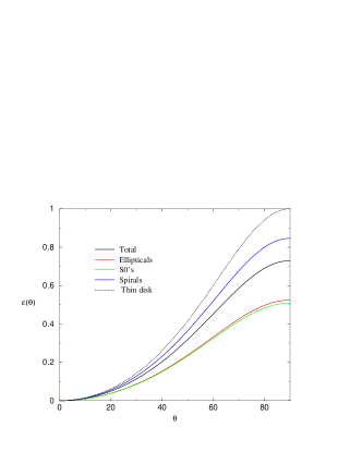
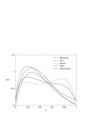
  Fig. 1.—: Left panel: The average ellipticities of the different morphological types of galaxies seen from a given angle $\theta$ with respect to the angular momentum vector. Also shown is the result for a sample with all types weighted by the observed fractions in the APM survey. All scale roughly as the thin disk case, Right panel: The distribution of ellipticities for the different morphological types based on the LBL intrinsic shape distributions. The differences between the LBL model and the fit from lensing surveys (dashed curve) could either be due to there being a different morphological mix in high redshift surveys or evolution in the intrinsic shape distributions, particularly for the spirals.

As can be seen in the left panel of Figure 1, $\bar{\epsilon}$ is different for each morphological type. The maxima, corresponding to when the galaxies are seen edge on, are significantly less than 1 due to the finite thicknesses of the galaxies. Interestingly, however, the dependence of $\bar{\epsilon}$ on $\theta$ for each of the morphological classes roughly scales identically to the disk case. That is, it is a good approximation to assume the same functional dependence on angle with an overall scaling:

$$|\bar{\epsilon}(\hat{L}_{z})|=\alpha{{1-\hat{L}_{z}^{2}}\over{1+\hat{L}_{z}^{2}}},$$ (15)

where $0<\alpha<1$ is a measure of the relative galaxy thickness. For the more realistic distributions, $\alpha$ ranges from 0.85 for spirals, down to around 0.5 for spheroids and ellipticals.

The mean redshift of the APM survey is $z_{m}=0.1$ and the composition of the sample is roughly 10% ellipticals, 25% spheroidals and 65% spirals. While these fractions might be representative of a local field sample, the redshift distribution of background galaxies of interest in lensing studies is considerably higher, so the morphological mix could be much different. To examine if this is the case, we plot both the distribution of ellipticities for the LBL populations and that measured for lensing studies

$${\cal{P}}(|\epsilon|)\propto|\epsilon|e^{-(|\epsilon|/0.3)^{1.15}}$$ (16)

(Brainerd et al. 1996; Ebbels et al. 2000), which is represented by the dashed curve on the right panel. The LBL distributions provide a poor fit to the results of the higher redshift field surveys. This could be due to two effects: either a different morphological mix or a different, perhaps non-Gaussian, distribution of intrinsic axis ratios for spirals. In addition, since the higher redshift surveys are more likely to be dominated by irregulars, the intrinsic shape distributions are expected to evolve.

Though we find that the LBL distributions on the whole provide a poor-fit to that from lensing studies, the inferred mean value for $|\bar{\epsilon}|$ is in good agreement. For a thin disk, $|\bar{\epsilon}|_{TD}=\pi/2-1$, so our simplified model has $|\bar{\epsilon}|=\alpha|\bar{\epsilon}|_{TD}=0.57\alpha.$ The mean of the measured ellipticity distribution (Eqn. 16) is 0.42, implying that $\alpha=0.73$. This is consistent with the mean value for $\alpha$ computed from the APM sample on the left panel of Figure 1. In the following sections, we will be explicitly computing correlations between the components of $\hat{\mathbf{L}}$ in order to calculate $\langle\epsilon\epsilon^{\prime}\rangle$ based on the definition in Eqn. (15).

3 Ellipticity and the tidal field

We wish to relate the ellipticity directly to the tidal field. The easiest way to do so is to consider the real and imaginary pieces of the distortion field separately:

$$\bar{\epsilon}_{+} = |\bar{\epsilon}|\cos(2\phi)=\alpha{{1-\hat{L}_{z}^{2}}\over{1+\hat{L}_{z}^{2}}}{{\hat{L}_{y}^{2}-\hat{L}_{x}^{2}}\over{\hat{L}_{y}^{2}+\hat{L}_{x}^{2}}}=\alpha{{\hat{L}_{y}^{2}-\hat{L}_{x}^{2}}\over{1+\hat{L}_{z}^{2}}}$$

$$\bar{\epsilon}_{\times} = |\bar{\epsilon}|\sin(2\phi)=\alpha{{1-\hat{L}_{z}^{2}}\over{1+\hat{L}_{z}^{2}}}{{\hat{L}_{y}\hat{L}_{x}}\over{\hat{L}_{y}^{2}+\hat{L}_{x}^{2}}}=\alpha{{\hat{L}_{y}\hat{L}_{x}}\over{1+\hat{L}_{z}^{2}}}.$$ (17)

When the observation frame coincides with the frame where the stress tensor is diagonal, $\langle\hat{L}_{y}\hat{L}_{x}\rangle=0$ and the expected distortion is purely real. Next we need to relate the angular momentum to the tidal field.

One central assumption in this work is that the expectation value of the angular momentum at a point is solely a function of the tidal tensor at that point. As the next step in calculating ellipticity correlations, we need to understand this relationship more quantitatively. That is, we need to know the probability of a given spin direction for a specified shear field, or effectively the form of ${\cal{P}}(\hat{\mathbf{L}}|{\mathbf{T}}).$ As discussed above, the angular momentum of a collapsing region is given by $L_{\alpha}\,=\,a^{2}(t)\,{\dot{D}}(t)\,\epsilon_{\alpha\beta\gamma}\,T_{\beta\sigma}\,I_{\sigma\gamma}.$ The crucial issue is how the moment of inertia for a collapsing object is related to the tidal field that it experiences. Unfortunately, this requires a precise understanding of what determines the region which eventually collapses into the galaxy, which in turn depends on the positions of nearby over-densities. This remains a major unsolved problem.

Catelan and Theuns (CT96a), studying the variance of the amplitude of the angular momentum of galaxies, initially assumed that the tidal tensor and the moment of inertia are entirely uncorrelated. However, since galaxies form preferentially at density peaks, CT96a also consider the suppression of angular momentum that arises around peaks in a Gaussian due to correlations between the inertia and the shear. In both of these cases, if one considers the frame where the inertia tensor is diagonal, the off-diagonal terms of the shear tensor are expected to be uncorrelated with the inertia tensor. However, around peaks the amplitude of these off-diagonal terms is suppressed, which results in lower angular momenta.

As we will show, the amplitude of the angular momentum has little effect on the magnitude of ellipticity correlations, which is chiefly determined by correlations in the directions of the spins. For simplicity, we will assume each component of the inertia tensor to be Gaussian distributed, so that the resulting distribution for the angular momentum given some shear tensor is also Gaussian distributed,

$${\cal{P}}({\mathbf{L}}|{\mathbf{T}})={1\over(2\pi)^{3\over 2}|{\cal{Q}}|^{1\over 2}}e^{-L_{\alpha}{\cal{Q}}_{\alpha\beta}^{-1}L_{\beta}/2}$$ (18)

where ${\cal{Q}}_{\alpha\beta}\equiv\langle L_{\alpha}L_{\beta}\rangle$ is the correlation matrix. In the frame where the shear is diagonal, the inertia tensor is uncorrelated with it and the correlation matrix has the form,

$$\langle L_{\alpha}L_{\beta}\rangle\propto\left[\begin{array}[]{ccc}(T_{33}-T_{22})^{2}&0&0\\ 0&(T_{11}-T_{33})^{2}&0\\ 0&0&(T_{22}-T_{11})^{2}\end{array}\right].$$ (22)

This has the same form in the peaks case studied by CT96a. The relation can be rewritten as

$$\langle L_{\alpha}L_{\beta}\rangle=\langle L^{2}\rangle\left({2\over 3}\delta_{\alpha\beta}-\hat{T}_{\alpha\gamma}\hat{T}_{\gamma\beta}\right),$$ (23)

where $\hat{T}$ is the unit normalized traceless tidal tensor ($\hat{T}_{\alpha\beta}\hat{T}_{\alpha\beta}=1$). Note that the angular momentum is independent of the trace of the tidal tensor, so we can consider $\hat{T}$ to be traceless without loss of generality. Our final expression for the ellipticity correlations will be independent of the proportionality factor $\langle L^{2}\rangle$, so uncertainties in this factor will be irrelevant here.

It has been argued that the approximations made by CT96a underestimate the correlations between the moment of inertia and the tidal field, and result in overestimating the angular momentum that is produced when compared to simulations. Lee and Pen (LP00) suggest that the CT96 approximations may do well in predicting the direction of the angular momentum, but not its amplitude. They consider the most general correlation between the shear and inertia tensors,

$$\langle{L}_{\alpha}{L}_{\beta}\rangle=\langle L^{2}\rangle\left({{1+a}\over 3}\delta_{\alpha\beta}-a\hat{T}_{\alpha\gamma}\hat{T}_{\gamma\beta}\right),$$ (24)

where $0\leq a\leq 1.$ The CT96a case of uncorrelated moment of inertia corresponds to $a=1$. In the extreme $a=0$ case, the direction of the angular momentum is random, independent of the tidal tensor. Ironically, stronger correlations between the moment of inertia and the tidal field make the direction of the expected angular momentum more, not less, random. The directions can be further perturbed by non-linear interactions, particularly if the magnitude of the angular momentum is small originally. LP00 investigate this in N-body simulations and find that the relation is best fit by $a=0.24$.

The distribution of the direction of the angular momentum vector is given by integrating over the amplitude of the momentum,

$${\cal{P}}(\hat{\mathbf{L}}|{\mathbf{T}})\, = \,\int\,L^{2}\,dL\,{\cal{P}}({\mathbf{L}}|{\mathbf{T}})$$

$$= \int_{0}^{\infty}\,L^{2}\,dL\,{1\over(2\pi)^{3\over 2}|{\cal{Q}}|^{1\over 2}}\,e^{-L^{2}\,\hat{L}_{\alpha}\,{\cal{Q}}_{\alpha\beta}^{-1}\,\hat{L}_{\beta}/2}$$

$$= {1\over 4\pi|\hat{\cal{Q}}|^{1\over 2}}(\hat{L}_{\alpha}\hat{\cal{Q}}_{\alpha\beta}^{-1}\hat{L}_{\beta})^{-{3\over 2}},$$ (26)

where $\hat{\cal{Q}}={\cal{Q}}/\langle L^{2}\rangle.$ The variance of the two point expectation value of the direction of the angular momentum is then

$$\langle\hat{L}_{\alpha}\hat{L}_{\beta}\rangle=\int d^{2}\hat{L}\,\,\hat{L}_{\alpha}\hat{L}_{\beta}{1\over 4\pi|\hat{\cal{Q}}|^{1\over 2}}(\hat{L}_{\alpha}\hat{\cal{Q}}_{\alpha\beta}^{-1}\hat{L}_{\beta})^{-{3\over 2}}.$$ (27)

As shown by LP00 and in Appendix B, for small $a$ this implies that

$$\langle\hat{L}_{\alpha}\hat{L}_{\beta}\rangle={\frac{1}{3}}(1-{\frac{3a}{5}})\delta_{\alpha\beta}+{\frac{3a}{5}}\hat{T}_{\alpha\gamma}\hat{T}_{\gamma\beta}.$$ (28)

Combining the above results, we can compute the average ellipticity for a given shear tensor at one point,

$$\bar{\epsilon}({\mathbf{T}}) = \int d{\mathbf{\hat{L}}}\,\epsilon({\mathbf{\hat{L}}})\,{\cal{P}}({\mathbf{\hat{L}}}|{\mathbf{T}})$$ (29)

$$= \alpha\int d^{2}{{\hat{L}}}\,\,{\frac{\sin^{2}\theta}{1+\cos^{2}\theta}}\,[\cos 2\phi+i\sin 2\phi]\,{1\over 4\pi|\hat{\cal{Q}}|^{1\over 2}}\,(\hat{L}_{\alpha}\hat{\cal{Q}}_{\alpha\beta}^{-1}\hat{L}_{\beta})^{-{3\over 2}}.$$

For small $a$, we can approximate $\hat{\cal{Q}}^{-1}\simeq{1\over 3}[\delta_{\alpha\beta}-a(\delta_{\alpha\beta}-3\hat{T}_{\alpha\gamma}\hat{T}_{\gamma\beta})]$. Therefore, $(\hat{L}_{\alpha}\hat{\cal{Q}}_{\alpha\beta}^{-1}\hat{L}_{\beta})^{-{3\over 2}}\simeq|\hat{\cal{Q}}|^{1\over 2}[1+{3a\over 2}-{9a\over 2}\hat{L}_{\alpha}\hat{L}_{\beta}\hat{T}_{\alpha\gamma}\hat{T}_{\gamma\beta}]$. Inserting this in the integral, by symmetry the surviving terms are

$$\bar{\epsilon}({\mathbf{T}}) = {-9a\alpha\over 8\pi}\int_{0}^{\pi}d\theta\,\frac{\sin^{5}\theta}{1+\cos^{2}\theta}\int_{0}^{2\pi}d\phi(\cos 2\phi+i\sin 2\phi)\,\left[\hat{T}_{1\gamma}\hat{T}_{\gamma 1}\cos^{2}\phi+\hat{T}_{2\gamma}\hat{T}_{\gamma 2}\sin^{2}\phi+2\hat{T}_{1\gamma}\hat{T}_{\gamma 2}\sin\phi\cos\phi\right]$$ (30)

$$= {-9a\alpha\over 8\pi}\int_{0}^{\pi}d\theta\,\frac{\sin^{5}\theta}{1+\cos^{2}\theta}\int_{0}^{2\pi}d\phi(\cos 2\phi+i\sin 2\phi)\,\left[\,A\,+\,B\cos 2\phi\,+\,C\sin 2\phi\,\right]$$

where $A={1\over 2}(\hat{T}_{1\gamma}\hat{T}_{\gamma 1}+\hat{T}_{2\gamma}\hat{T}_{\gamma 2})$, $B={1\over 2}(\hat{T}_{1\gamma}\hat{T}_{\gamma 1}-\hat{T}_{2\gamma}\hat{T}_{\gamma 2})$ and $C=\hat{T}_{1\gamma}\hat{T}_{\gamma 2}.$ Finally, using $\int_{0}^{\pi/2}d\theta\,\frac{\sin^{5}\theta}{1+\cos^{2}\theta}\,=\,\pi-8/3$, we find that the integral of Eqn. (26) evaluates to

$$\bar{\epsilon}({\mathbf{T}}) = \bar{\epsilon}_{+}({\mathbf{T}})+i\bar{\epsilon}_{\times}({\mathbf{T}})=a\alpha(6-{9\pi\over 4})\,[\,{1\over 2}(\hat{T}_{1\gamma}\hat{T}_{\gamma 1}-\hat{T}_{2\gamma}\hat{T}_{\gamma 2})\,+\,i\hat{T}_{1\gamma}\hat{T}_{\gamma 2}\,].$$ (31)

The numerical factor, ${9\pi\over 4}-6$, is very nearly unity and we shall drop it for convenience here. Thus, the average ellipticity for a given tidal field is quadratic in the tidal field and is suppressed both by a factor due to the finite thicknesses of the galaxies ($\alpha$) and by the randomization of the angular momentum vector ($a$).

4 Correlations in the Tidal Field

In the previous section we related the ellipticity to the tidal field, and here we calculate the moments of the tidal field required to derive ellipticity correlations. Since the tidal tensor is the second derivative of the gravitational potential, its statistical properties are directly related to those of the matter density. We assume that the underlying density field is Gaussian distributed, which implies that the tidal field is also Gaussian. However, the unit normalized tidal field which is of relevance to us will not be Gaussian distributed.

Knowing the full statistics of the tidal field, it is possible to calculate expectation values of observables such as the ellipticity correlation $\langle\epsilon\epsilon{{}^{\prime*}}\rangle=\int d{\mathbf{T}}d{\mathbf{T}}^{\prime}\bar{\epsilon}({\mathbf{T}})\bar{\epsilon}^{*}({\mathbf{T}}^{\prime}){\cal{P}}({\mathbf{T}},{\mathbf{T}}^{\prime}).$ Since the ellipticity is quadratic in $\hat{\mathbf{T}}$, we need to compute linear and quadratic two point functions of the normalized shear field, $\langle\hat{\mathbf{T}}\hat{\mathbf{T}}^{\prime}\rangle$ and $\langle\hat{\mathbf{T}}\hat{\mathbf{T}}\hat{\mathbf{T}}^{\prime}\hat{\mathbf{T}}^{\prime}\rangle$ respectively. We first compute the correlations of ${\mathbf{T}}$ which are necessary to evaluate these moments.

4.1 Correlations of ${\mathbf{T}}$

To begin, we compute the two point expectation value of the tidal tensor in terms of the power spectrum of fluctuations. A Fourier expansion of the shear tensor yields,

$$T_{\alpha\beta}({\mathbf{x}})\,=\,-\int\,d^{3}{\mathbf{k}}\,k_{\alpha}\,k_{\beta}\,\Psi({\mathbf{k}})\,e^{i{\mathbf{k}}\cdot{\mathbf{x}}},$$ (32)

where $\Psi({\mathbf{k}})$ is the Fourier transform of the gravitational potential, which has a power spectrum defined as,

$$\langle{\Psi(\mathbf{k})\,\Psi(\mathbf{k}^{\prime})}\rangle\,=\,\delta_{\rm D}({\mathbf{k}}-{\mathbf{k}^{\prime}})\,P_{\Psi}(k).$$ (33)

¿From this, it is straight forward to calculate the two-point correlation function of the tidal tensor,

$$C_{\alpha\beta\gamma\sigma}({\mathbf{r}}) \equiv \langle T_{\alpha\beta}({\mathbf{x}})\,T_{\gamma\sigma}({\mathbf{x}^{{}^{\prime}}})\rangle\,=\,\int\,d^{3}{\mathbf{k}}\,k_{\alpha}\,k_{\beta}\,k_{\gamma}\,k_{\sigma}\,P_{\Psi}(k)\,e^{i{\mathbf{k}}\cdot{\mathbf{r}}},$$ (34)

where the separation is ${\mathbf{r}}={\mathbf{x}}-{\mathbf{x}^{\prime}}$.

To evaluate the correlation function, it is useful to relate Fourier space components back to the real space derivatives via $ik_{\alpha}\equiv{\partial_{\alpha}}.$ Thus, we have

$$C_{\alpha\beta\gamma\sigma}({\mathbf{r}})\, = \,\partial_{\alpha}\partial_{\beta}\partial_{\gamma}\partial_{\sigma}\int\,d^{3}{\mathbf{k}}\,P_{\Psi}(k)\,e^{i{\mathbf{k}}\cdot{\mathbf{r}}}$$ (35)

$$= \,2\pi\partial_{\alpha}\partial_{\beta}\partial_{\gamma}\partial_{\sigma}\int\,dk\,k^{2}\,P_{\Psi}(k)\,j_{0}(kr).$$

Here we have performed the integration over the angular directions of the Fourier modes, and $j_{0}(kr)=\sin kr/kr$ is the zeroth order spherical Bessel function.

It is useful to rewrite the derivatives as ${\partial_{\alpha}}=({dr/dx_{\alpha}})({d/dr})=x_{\alpha}D$, where the operator $D\equiv(1/r)(d/dr)$. Using the identity ${\partial_{\alpha}}x_{\beta}=\delta_{\alpha\beta},$ we find

$$C_{\alpha\beta\gamma\sigma}({\mathbf{r}}) = \,2\pi\partial_{\alpha}\partial_{\beta}\int\,dk\,k^{2}\,P_{\Psi}(k)\,(\delta_{\gamma\sigma}\,D[j_{0}(kr)]\,+\,x_{\gamma}\,x_{\sigma}\,D^{2}[j_{0}(kr)])$$ (36)

$$= \,2\pi[\delta_{\alpha\beta}\delta_{\gamma\sigma}\,+\,\delta_{\alpha\gamma}\delta_{\beta\sigma}\,+\,\delta_{\alpha\sigma}\delta_{\beta\gamma}]\int\,dk\,k^{2}\,P_{\Psi}(k)\,D^{2}[j_{0}(kr)]$$

$$+ \,2\pi[r_{\alpha}r_{\beta}\delta_{\gamma\sigma}+r_{\alpha}r_{\gamma}\delta_{\beta\sigma}+r_{\alpha}r_{\sigma}\delta_{\beta\gamma}+r_{\beta}r_{\gamma}\delta_{\alpha\sigma}+r_{\beta}r_{\sigma}\delta_{\alpha\gamma}+r_{\gamma}r_{\sigma}\delta_{\alpha\beta}]\int\,dk\,k^{2}\,P_{\Psi}(k)\,D^{3}[j_{0}(kr)]$$

$$+\,2\pi r_{\alpha}r_{\beta}r_{\gamma}r_{\sigma}\,\int\,dk\,k^{2}\,P_{\Psi}(k)\,D^{4}[j_{0}(kr)].$$

It is possible to use Poisson’s equation to substitute the power spectrum of the potential with that of the density, $k^{4}P_{\Psi}(k)=P_{\delta}(k)$, in units where $4\pi G\rho_{0}=1$ and $G$ is the gravitational constant. Using the identity $D^{n}\,j_{0}(r)=(-1)^{n}\,r^{-n}\,j_{n}(r)$, the above simplifies to

$$C_{\alpha\beta\gamma\sigma}({\mathbf{r}}) = [\delta_{\alpha\beta}\delta_{\gamma\sigma}+\delta_{\alpha\gamma}\delta_{\beta\sigma}+\delta_{\alpha\sigma}\delta_{\beta\gamma}]\zeta_{2}(r)+\hat{r}_{\alpha}\hat{r}_{\beta}\hat{r}_{\gamma}\hat{r}_{\sigma}\,\zeta_{4}(r)$$ (37)

$$+ [\hat{r}_{\alpha}\hat{r}_{\beta}\delta_{\gamma\sigma}\,+\hat{r}_{\alpha}\hat{r}_{\gamma}\delta_{\beta\sigma}\,+\hat{r}_{\alpha}\hat{r}_{\sigma}\delta_{\beta\gamma}\,+\hat{r}_{\beta}\hat{r}_{\gamma}\delta_{\alpha\sigma}+\hat{r}_{\beta}\hat{r}_{\sigma}\delta_{\alpha\gamma}+\hat{r}_{\gamma}\hat{r}_{\sigma}\delta_{\alpha\beta}]\,\zeta_{3}(r),$$

where

$$\zeta_{n}(r)=(-1)^{n}\,\frac{2\pi}{r^{4-n}}\int{dk\,k^{n-2}\,j_{n}(kr)\,P_{\delta}(k)},$$ (38)

and $j_{n}(kr)$ is the $n^{th}$ spherical Bessel function. This is identical to the expression derived in LP00, wherein it was shown that these $\zeta$ functions are related to the density correlation function, $\xi(r)=\int dk\,k^{2}P_{\delta}(k)j_{0}(kr)$, and integrals of it.

If the density field is smoothed, its correlation function levels off as $r\rightarrow 0$. In this limit, $\zeta_{3}$ and $\zeta_{4}\rightarrow 0$ and the above expression reduces to

$$C_{\alpha\beta\gamma\sigma}(0)=\zeta_{2}(0)[\delta_{\alpha\beta}\delta_{\gamma\sigma}+\delta_{\alpha\gamma}\delta_{\beta\sigma}+\delta_{\alpha\sigma}\delta_{\beta\gamma}].$$ (39)

Since $\zeta_{2}(0)=\xi(0)/15$, this corresponds precisely to the variance of the tidal field found by CT96a (equation (38) in Appendix A.) The correlation function simplifies dramatically when averaging over directions ${\hat{r}}$,

$$C_{\alpha\beta\gamma\sigma}(r)\equiv\frac{1}{4\pi}\,\int\,d^{2}{\hat{r}}\,C_{\alpha\beta\gamma\sigma}({\mathbf{r}})\,=\,\frac{1}{15}\xi(r)\,[\delta_{\alpha\beta}\delta_{\gamma\sigma}+\delta_{\alpha\gamma}\delta_{\beta\sigma}+\delta_{\alpha\sigma}\delta_{\beta\gamma}].$$ (40)

This is useful when the correlation length is much smaller than the depth of the survey.

4.2 Correlations of $\hat{\mathbf{T}}$

In this sub-section, we calculate the two and four point moments of the unit normalized traceless tidal field, $\hat{\mathbf{T}}$. Since ${\mathbf{T}}$ is not Gaussian distributed, these moments are not necessarily simply related. In the next sub-section, we use these results to derive the final ellipticity correlation.

For simplicity of notation, it is useful to treat the six degrees of freedom in the shear tensor as a vector, which we shall denote with capital Roman subscripts, ${\mathbf{T}}=(T_{11},T_{22},T_{33},T_{12},T_{13},T_{23})$. While using this notation, it is important to remember that the shear transforms as a tensor under rotations, rather than as a vector. To further simplify the notation, we shall write the shear field at a displacement $\mathbf{r}$ from the origin as $\mathbf{T}^{\prime}$. Thus in this notation, the correlation matrix becomes a six by six matrix, $\langle T_{A}T_{B}^{\prime}\rangle=[C_{\mathbf{r}}]_{AB}$.

Since the tidal field is Gaussian, with a two-point correlation matrix given by $C$, we can write the expectation value for an observable like $\hat{T}_{A}\hat{T}_{B}$ as,

$$\langle{\hat{T}_{A}}\,{\hat{T}_{B}}^{\prime}\rangle\,=\,\int\,\frac{d^{6}Td^{6}T^{\prime}}{{|C|^{1/2}}{(2\,\pi)^{6}}}{\hat{T}}_{A}\,{\hat{T}_{B}}^{\prime}\,e^{-\frac{1}{2}{\vec{T}^{T}}{C^{-1}}{\vec{T}}}\,$$ (41)

where ${\vec{T}}=({\mathbf{T}},{\mathbf{T}}^{\prime})$. The matrix $C$ has the following block diagonal form,

$${C}\,=\,\left[\begin{array}[]{cc}C_{0}&C_{\mathbf{r}}\\ C_{\mathbf{r}}&C_{0}\end{array}\right],$$ (44)

where $C_{0}$ is the zero-lag correlation matrix and $C_{\mathbf{r}}$ contains the two point correlations. For galaxies that are separated by distances greater than the smoothing scale, we can assume that $C_{\mathbf{r}}\,\ll\,C_{0}$ and expand in powers of $C_{\mathbf{r}}C^{-1}_{0}$ to invert $C$ to second order:

$${C^{-1}}\,\simeq\,\left[\begin{array}[]{cc}{C^{-1}_{0}(1+C_{\mathbf{r}}C^{-1}_{0}C_{\mathbf{r}}C^{-1}_{0})}&{-C^{-1}_{0}C_{\mathbf{r}}C^{-1}_{0}}\\ {-C^{-1}_{0}C_{\mathbf{r}}C^{-1}_{0}}&{C^{-1}_{0}(1+C_{\mathbf{r}}C^{-1}_{0}C_{\mathbf{r}}C^{-1}_{0})}\end{array}\right].$$ (47)

We perform a Taylor expansion of the exponential,

$$\exp[{-\frac{1}{2}{\vec{T}^{T}}{C^{-1}}{\vec{T}}}]\simeq[1+T\,C^{-1}_{0}\,C_{\mathbf{r}}\,C^{-1}_{0}\,T^{\prime}+\frac{1}{2}(T\,C^{-1}_{0}\,C_{\mathbf{r}}\,C^{-1}_{0}\,T^{\prime})^{2}+\,\ldots\,\,]\exp[-\frac{1}{2}(T\,C^{-1}_{0}\,T+T^{\prime}\,C^{-1}_{0}\,T^{\prime})].$$ (48)

To evaluate the linear two point function of $\hat{\mathbf{T}}$, we must keep terms to first order in $C_{\mathbf{r}}C^{-1}_{0}$. The expectation value can then be written as,

$$\langle{\hat{T}_{A}\,{\hat{T}_{B}}}^{\prime}\rangle\, = \,\int\,\frac{d^{6}T\,d^{6}T^{\prime}}{{|C_{0}|}{(2\,\pi)^{6}}}{\hat{T}_{A}}\,{\hat{T}_{B}}^{\prime}[T\,C^{-1}_{0}C_{\mathbf{r}}C^{-1}_{0}\,T^{\prime}]e^{{-\frac{1}{2}(T\,C^{-1}_{0}\,T+T^{\prime}\,C^{-1}_{0}\,T^{\prime})}}\,$$ (49)

$$= \langle{\hat{T}_{A}}\,{T_{C}}\rangle\,[C^{-1}_{0}C_{\mathbf{r}}C^{-1}_{0}]_{CD}\,\langle{\hat{T}_{B}^{\prime}}\,{T_{D}}^{\prime}\rangle,$$

where

$$\langle{\hat{T}_{A}}\,{T_{B}}\rangle\,\equiv\,\int{\frac{d^{6}T}{(2\pi)^{3}|C_{0}|^{1/2}}}{\hat{T}_{A}}\,{T_{B}}\,e^{{-\frac{1}{2}({T\,C^{-1}_{0}\,T})}},$$ (50)

is proportional to the mean magnitude of the tidal field. This is evaluated in Appendix C by transforming variables, ${\cal{T}}_{A}\equiv R_{AA^{\prime}}T_{A^{\prime}}$, to a basis in which the correlation function is proportional to the unit matrix. Using the results derived there, the linear two point function is shown to be,

$$\langle{\hat{T}_{A}\,{\hat{T}_{B}}}^{\prime}\rangle\, = \frac{64}{225\pi\zeta_{2}(0)}[\tilde{C}_{\mathbf{r}}]_{AB}$$ (51)

where $\tilde{C}_{\mathbf{r}}$ is the correlation function of the traceless part of the tidal field. Though this was evaluated in the large separation limit, its value at zero lag is very close to the exact result.

The quadratic two point function of $\hat{\mathbf{T}}$ is evaluated in an analogous way, except here we must keep terms to second order in $C_{\mathbf{r}}C^{-1}_{0}$. Making this substitution, the quadratic two point function is

$$\langle{\hat{T}_{A}}\,{\hat{T}_{B}}{\hat{T}_{C}}^{\prime}{\hat{T}_{D}}^{\prime}\rangle\, = \,\int\,\frac{d^{6}Td^{6}T^{\prime}}{{|C|^{1/2}}{(2\,\pi)^{6}}}{\hat{T}}_{A}\,{\hat{T}_{B}}{\hat{T}_{C}}^{\prime}{\hat{T}_{D}}^{\prime}\,e^{-\frac{1}{2}{\vec{T}^{T}}{C^{-1}}{\vec{T}}}\,$$ (52)

$$= \langle{\hat{T}_{A}}\,{\hat{T}_{B}}\rangle\langle{\hat{T}_{C}}^{\prime}{\hat{T}_{D}}^{\prime}\rangle\,+\frac{1}{2}\langle{\hat{T}_{A}}\,{\hat{T}_{B}}{T_{E}}{T_{F}}\rangle\,\langle{\hat{T}_{C}}\,{\hat{T}_{D}}{T_{G}}{T_{H}}\rangle\,[C^{-1}_{0}\,C_{\mathbf{r}}\,C^{-1}_{0}]_{EG}[C^{-1}_{0}\,C_{\mathbf{r}}\,C^{-1}_{0}]_{FH}.$$

As before, the expectation value of

$$\langle{\hat{T}}_{A}\,{\hat{T}}_{B}T_{C}T_{D}\rangle\,=\,\int{\frac{d^{6}T}{(2\pi)^{3}|C_{0}|^{1/2}}}{\hat{T}_{A}}\,{\hat{{T}}_{B}}{T}_{C}{T}_{D}\,e^{{-\frac{1}{2}({T\,C^{-1}_{0}\,T})}}$$ (53)

is computed in the transformed basis and is derived in Appendix C. The final form of the quadratic two point function is then

$$\langle{\hat{T}_{A}}\,{\hat{T}_{B}}{\hat{T}_{C}}^{\prime}{\hat{T}}_{D}^{\prime}\rangle\, = \left(\frac{1}{14\zeta_{2}(0)}\right)^{2}\left[[\tilde{C}_{\mathbf{r}}]_{AC}[\tilde{{C}}_{\mathbf{r}}]_{BD}+[\tilde{C}_{\mathbf{r}}]_{AD}[\tilde{C}_{\mathbf{r}}]_{BC}\right]+\,{\rm local\,terms},$$ (54)

where $\tilde{C}_{\mathbf{r}}$ is defined as above. The local terms correspond to the reducible parts of this fourth order moment and do not contribute to the ellipticity correlation.

4.3 Correlations of the Ellipticity

Using the results derived earlier, we are finally in a position to calculate ellipticity correlations. Recall that the ellipticity correlations are given by

$$\langle\epsilon\epsilon^{\prime*}\rangle = \int d\tilde{\mathbf{T}}d\tilde{\mathbf{T}}^{\prime}\bar{\epsilon}(\tilde{\mathbf{T}})\bar{\epsilon}^{*}(\tilde{\mathbf{T}}^{\prime}){\cal{P}}(\tilde{\mathbf{T}},\tilde{\mathbf{T}}^{\prime})$$ (55)

$$\simeq a^{2}\alpha^{2}\langle[\,{1\over 2}(\hat{T}_{1\gamma}\hat{T}_{\gamma 1}-\hat{T}_{2\gamma}\hat{T}_{\gamma 2})\,+\,i\hat{T}_{1\gamma}\hat{T}_{\gamma 2}\,][\,{1\over 2}(\hat{T}_{1\sigma}^{\prime}\hat{T}_{\sigma 1}^{\prime}-\hat{T}_{2\sigma}^{\prime}\hat{T}_{\sigma 2}^{\prime})\,-\,i\hat{T}_{1\sigma}^{\prime}\hat{T}_{\sigma 2}^{\prime}\,]\rangle.$$

We choose the separation vector $\mathbf{r}$ to lie in the $x-z$ plane at an angle $\theta$ from the line-of-sight which we assume to be parallel to the $z-$axis. This choice implies that frames in which the ellipticities are measured lie parallel to the projected separation.

Inserting equation (54) the two non-zero components of the ellipticity correlation are,

$$\langle\epsilon_{+}\epsilon_{+}^{\prime}\rangle= \frac{a^{2}\alpha^{2}}{144}({\frac{1}{14\zeta_{2}(0)}})^{2} [336\,\zeta_{2}^{2}(r)+472\,\zeta_{2}(r)\,\zeta_{3}(r)+155\,\zeta_{3}^{2}(r)+58\,\zeta_{2}(r)\,\zeta_{4}(r)+26\,\zeta_{3}(r)\,\zeta_{4}(r)+3\,\zeta_{4}^{2}(r)$$ (56)

$$+\,4\left(18\,\zeta_{2}(r)\,\zeta_{3}(r)-7\,\zeta_{3}^{2}(r)-8\,\zeta_{3}(r)\,\zeta_{4}(r)-\,\zeta_{4}^{2}(r)\right)\,\cos 2\,{\theta}$$

$$+\,\left(17\,\zeta_{3}^{2}(r)+6\,\zeta_{2}(r)\,\zeta_{4}(r)+6\,\zeta_{3}(r)\,\zeta_{4}(r)+\,\zeta_{4}^{2}(r)\right)\,\cos 4\,{\theta}],$$

and

$$\langle\epsilon_{\times}\epsilon_{\times}^{\prime}\rangle= \frac{a^{2}\alpha^{2}}{18}({\frac{1}{14\zeta_{2}(0)}})^{2} [42\,\zeta_{2}^{2}(r)+59\,\zeta_{2}(r)\,\zeta_{3}(r)+13\,\zeta_{3}^{2}(r)+5\,\zeta_{2}(r)\,\zeta_{4}(r)+\zeta_{3}(r)\,\zeta_{4}(r)$$ (57)

$$+\left(9\,\zeta_{2}(r)\,\zeta_{3}(r)+5\,\zeta_{3}^{2}(r)+3\,\zeta_{2}(r)\,\zeta_{4}(r)-\,\zeta_{3}(r)\,\zeta_{4}(r)\right)\cos 2\,{\theta}].$$

For a simple model with $\xi(r)\propto 1/r$, $\langle\epsilon_{+}\epsilon_{+}^{\prime}\rangle$ and $\langle\epsilon_{\times}\epsilon_{\times}^{\prime}\rangle$ are plotted in Figure 2, computed assuming top-hat smoothing on a 1 $h^{-1}$ Mpc scale.

These functions are explicitly anisotropic and depend on the angle between $\mathbf{r}$ and the line of sight. Much of the angular dependence can be understood intuitively by considering the symmetries of the problem. When the line of sight is parallel to $\mathbf{r}$ ($\theta=0$), there is no longer a distinction between $\epsilon_{+}$ and $\epsilon_{\times}$, so that $\langle\epsilon_{+}\epsilon_{+}^{\prime}\rangle$ and $\langle\epsilon_{\times}\epsilon_{\times}^{\prime}\rangle$ are identical. In addition these correlations are invariant under the transformations $\theta\rightarrow-\theta$ and $\theta\rightarrow\pi-\theta$ so that the only surviving terms are either constant or proportional to $\cos 2\theta$ or $\cos 4\theta$. This anisotropy is demonstrated in the right panel of Figure 2.

Asymptotically at large $r$, the angle averaged behavior is approximately

$$\langle\epsilon\epsilon{{}^{\prime*}}\rangle\simeq{a^{2}\alpha^{2}\over 84}{\xi^{2}(r)\over\xi^{2}(0)}.$$ (58)

This is very close to the exact expression at large $r$, as is shown in the left panel of Figure 2. The factor of 1/84 has been derived for large separations. At zero lag, it can be computed directly from the fourth moment of the unit normalized traceless shear tensor and is found to be 1/60.

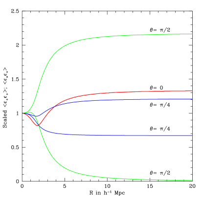
  Fig. 2.—: Left panel: The computed three dimensional ellipticity correlation function averaged over angles and plotted as a function of separation. The signal is appreciable at separations smaller than the smoothing scale ($<1$ Mpc) and falls off as $\xi^{2}(r)$. For comparison we have plotted the exact derived function [solid curve] against the approximation of Equation (58) [dashed curve]. Right panel: The expectation value of the two components of the two point ellipticity correlation $\langle\epsilon_{+}\epsilon_{+}\rangle$ and $\langle\epsilon_{\times}\epsilon_{\times}\rangle$ divided by the approximate curve (solid curve of left panel) for various values of the viewing angle $\theta=0,\pi/4$ and $\pi/2$ are shown. Note that the 2 components are equal for $\theta=0$.

4.4 Peaks in a Gaussian field

Galaxies do not form at random positions, but at peaks of the density field (Bardeen et al. 1986). It is possible that this sampling could bias the expected correlation of galaxy ellipticities since our analytic correlations have been computed for random points. We examine such a potential bias using numerical realizations of Gaussian fields, and also use these to check the validity of our analytic results.

We create realizations of Gaussian fields on a 512³ grid with a power spectrum $P_{\delta}\propto k^{-2},$ corresponding to a density correlation which falls off as $1/r.$ The density field is smoothed with a spherical top-hat filter of approximately four grid units. Peaks are identified as positions where the density field exceeds the value at each of its six nearest neighbors. The tidal field is calculated at each point using differencing. At each point, we compute and subtract the trace and finally unit normalize the tidal tensor.

We checked first that the moments of the normalized tidal field match our analytic expectations at zero lag. For example, we can analytically calculate the variance of one component of the tidal tensor, $\langle\hat{T}_{xx}^{2}\rangle$. From isotropy, this can be shown to be $2/15$, which we have verified in the realizations. We have also checked numerically other exact quadratic and quartic relations such as $\langle\hat{T}_{xy}^{2}\rangle=1/10$, $\langle\hat{T}_{xx}^{4}\rangle=4/105$ and $\langle\hat{T}_{xx}^{2}\hat{T}_{xy}^{2}\rangle=1/105.$

Using the definition in Equation (48), we compute the correlation function of the (angle averaged) ellipticity on the grid both for peaks and random field points, assuming $a=\alpha=1$. These are compared with the derived analytic results in Figure 3. The correlation function for the peaks ($\sim$ 70,000 in the box) and the field points are in excellent agreement for both small and large separations. At zero lag, they both asymptote to the analytic result of $1/60$ (marked in Figure 3 by the horizontal long-dashed line). The maximum deviation occurs around the smoothing scale and is of the order of 10%. This implies that while peaks might preferentially be sites of galaxy formation, as far as intrinsic ellipticity correlations are concerned, there is no substantial bias between peaks and random field points.

The numerical correlation function starts dropping below the exact analytic expectation (plotted as the solid curve) for large separations. This is due to missing large-scale power on the grid: an analytic calculation that incorporates the same lack of power on large scales as the grid is shown as the dashed line. Its agreement with the numerical results demonstrates that the steeper fall off of the numerical estimates is indeed an artifact of the finite box size. Clearly this is a worry for all numerical computations of the ellipticity correlation function. Additionally, on separations smaller than the smoothing scale, our analytic estimates fall below the numerical results and the exact values derived from the one point moments. This discrepancy arises because the approximation we made in computing the analytic results, $C(r)/C(0)\ll 1,$ is invalid on small scales.

  Fig. 3.—: The angle averaged ellipticity correlations from Gaussian field realizations on a $512^{3}$ grid compared to the analytic results. The correlations at peaks of the density field (shown as solid squares) appear to match well with the results from random positions (the dot-dashed line). At zero-lag they both asymptote to the exact result ($1/60$) shown by the horizontal dot-dashed line. The full analytic correlations (solid curves) as well as the analytic estimate where the large scale power has been removed (dashed curve) to account for the finite size of the realizations are both shown. These are not valid below the smoothing scale. The analytic results match well in the region where they are valid, i. e. at scales larger than the smoothing length, but note the importance of large-scale power (here we have set $a=\alpha=1$).

5 The projected correlation functions

Up to now we have been focusing on the three dimensional ellipticity correlation function. While this is in principle observable (Pen et al. 2000), weak lensing studies usually consider the ellipticity correlation projected onto the sky. The projection of the intrinsic signal will enable us to compare directly with weak lensing estimates and judge its importance as a possible contaminant for these measurements.

5.1 Limber’s equation

We begin by making some general comments about the basis dependence of the two dimensional correlation functions. Previously, we calculated the three dimensional correlation functions in a special basis, one where the separation vector was coplanar with one of the axes used to define the ellipticity. We showed that the ellipticity correlations in this basis were functions only of the 3-D separation and the angle $\cos\theta=\hat{\mathbf{z}}\cdot\hat{\mathbf{r}}$. In two dimensions, this basis is equivalent to taking one axis vector to be parallel to the 2-D separation $\vec{r}$. In this special basis, which hereafter will be denoted by the superscript $r$, the ellipticity correlations will only be functions of the distance between the two points. We will denote these functions as,

$$\xi_{+}(|\vec{r}|)\equiv\langle\epsilon^{r}_{+}({\vec{x}})\epsilon^{r}_{+}({\vec{x}+\vec{r}})\rangle;\,\,\xi_{\times}(|\vec{r}|)\equiv\langle\epsilon^{r}_{\times}({\vec{x}})\epsilon^{r}_{\times}({\vec{x}+\vec{r}})\rangle.$$ (59)

The cross correlation, $\langle\epsilon^{r}_{+}({\vec{x}})\epsilon_{\times}^{r}({\vec{x}+\vec{r}})\rangle,$ is zero due to parity ($x\rightarrow-x$) invariance.

The basis for these correlation functions depends on the separation vector, and thus on which pair of galaxies one is considering. It is often useful to work in a fixed basis on the sky for the ellipticities. The ellipticity measured in an arbitrary basis with an angle $\phi$ relative to the separation vector is given by:

$$\epsilon_{+} = \epsilon_{+}^{r}\cos 2\phi-\epsilon_{\times}^{r}\sin 2\phi;$$

$$\epsilon_{\times} = \epsilon_{+}^{r}\sin 2\phi+\epsilon_{\times}^{r}\cos 2\phi.$$ (60)

In such a fixed basis, the correlation function depends on $\phi$ as,

$$C_{1}(|\vec{r}|,\phi)\equiv\langle\epsilon_{+}\epsilon_{+}^{\prime}\rangle = \xi_{+}(|\vec{r}|)\cos^{2}2\phi\,+\,\xi_{\times}(|\vec{r}|)\sin^{2}2\phi$$

$$C_{2}(|\vec{r}|,\phi)\equiv\langle\epsilon_{\times}\epsilon_{\times}^{\prime}\rangle = \xi_{\times}(|\vec{r}|)\cos^{2}2\phi\,+\,\xi_{+}(|\vec{r}|)\sin^{2}2\phi,$$ (61)

for all pairs separated by $|\vec{r}|$ at an angle of $\phi$ with respect to the chosen basis. The sum of these is a function of the separation only, while the difference has a simple dependence on $\phi$:

$$C_{1}(|\vec{r}|,\phi)+C_{2}(|\vec{r}|,\phi)=\xi_{+}(|\vec{r}|)+\xi_{\times}(|\vec{r}|);\,\,\,C_{1}(|\vec{r}|,\phi)-C_{2}(|\vec{r}|,\phi)=[\xi_{+}(|\vec{r}|)-\xi_{\times}(|\vec{r}|)]\cos 4\phi.$$ (62)

Recent measurements of the shear from weak lensing have focused on the variance of the magnitude of the ellipticity averaged over a patch, which depends only on the sum.

We next consider the projection into two dimensions and use an approach similar to that used by Heavens et al. (2000) and Croft & Metzler (2000). Assuming that we are working on a small area of the sky, the observed patch of sky is approximated by a plane. The projection uses Limber’s equation to take into account the clustering of galaxies,

$$\xi_{+}(|\vec{r}|)\, = \,\frac{\int z_{1}^{2}z_{2}^{2}dz_{1}dz_{2}\psi(z_{1})\,\psi(z_{2})\,[1+\xi_{gg}(r)]\,\langle\epsilon_{+}(\mathbf{x_{1}})\epsilon_{+}(\mathbf{x_{2}})\rangle}{\int z_{1}^{2}z_{2}^{2}dz_{1}dz_{2}\psi(z_{1})\,\psi(z_{2})\,[1+\xi_{gg}(r)]}$$

$$\xi_{\times}(|\vec{r}|)\, = \,\frac{\int z_{1}^{2}z_{2}^{2}dz_{1}dz_{2}\psi(z_{1})\,\psi(z_{2})\,[1+\xi_{gg}(r)]\,\langle\epsilon_{\times}(\mathbf{x_{1}})\epsilon_{\times}(\mathbf{x_{2}})\rangle}{\int z_{1}^{2}z_{2}^{2}dz_{1}dz_{2}\psi(z_{1})\,\psi(z_{2})\,[1+\xi_{gg}(r)]},$$ (63)

where $|\vec{r}|^{2}=(r^{2}-(z_{1}-z_{2})^{2})$, $\psi(z)$ is the observational selection function and $\xi_{gg}(r)$ is the galaxy-galaxy correlation function.

Note that while the ellipticity correlation function is calculated in Lagrangian coordinates, the projection is performed in Eulerian space. The Eulerian separations will differ from the Lagrangian ones due to peculiar velocities of galaxies, which we have ignored here. For galaxies near each other, the Eulerian separations will in general be smaller than the corresponding Lagrangian ones. This will result in a suppression of the intrinsic projected ellipticity correlations. We expect this effect to be small at large separations, but it could be significant closer in.

  Fig. 4.—: The projected 2-d ellipticity correlation functions, $\xi_{+}$ and $\xi_{\times}$, for various values of the median redshift of the distribution of galaxies. Here we have assumed the galaxies are well described by thin disks and are perfectly aligned with the linear predictions ($a=\alpha=1$.) but deviate at larger separation. Both increase strongly with decreasing redshift, roughly proportional to $z_{m}^{-2}$.

5.2 Qualitative Features

In Figure 4 we plot the projected correlation function calculated for the simple model in which the density correlation falls off as $1/r$. We have assumed a top-hat smoothing scale of 1 $h^{-1}$Mpc. The clustering term is taken to be of the form $\xi_{\rm gg}=(r/R_{s})^{-\beta}$ where $R_{s}=5h^{-1}$ Mpc is the clustering scale and $\beta=1.8$ (Loveday et al. 1992). Finally, following Heavens et al., the selection function is taken to be $\psi(z)=e^{-(z/z_{0})^{1.5}}$ which has a mean redshift of $z_{m}=1.4z_{0}$. In the figure we plot the functions $\xi_{+}$ and $\xi_{\times}$ for $a=\alpha=1$. They are nearly identical at small angular scales, but deviate at larger separation.

The qualitative features of these correlation functions can be understood by looking at the various scales in the problem: $R_{m}$, the mean depth of the survey; $R_{s}$, the clustering length of galaxies and $R_{0}$, the smoothing scale. If the density correlation function falls off as $1/r$, the three dimensional ellipticity correlation scales as $\xi_{+}\simeq\xi_{\times}\simeq a^{2}\alpha^{2}R_{0}^{2}/84(R_{0}^{2}+r^{2}),$ where we have used the approximation from Eqn. (58). Both the numerator and the denominator of Equation (63) contain a clustering term, which dominates at small angular separations and a mean contribution.

The denominator in Limber’s equation is essentially the average number of galaxies within an angular distance $\theta$ from a given galaxy out to the volume of the survey. At large separations, the denominator scales as the volume squared, or $R_{m}^{6}$. Corrections from clustering are of order $R_{m}^{6}(R_{s}/R_{m})^{\beta}\theta^{1-\beta},$ which become important at angles $\theta<(R_{s}/R_{m})^{\beta\over\beta-1}.$ For a survey with median redshift $z_{m}\sim 1$, this occurs at about 2 arc seconds. For a shallower survey with $z_{m}\sim 0.1$, this occurs at much larger scales, of order a few arc minutes.

The numerator in Limber’s equation is the projected ellipticity correlation function, weighted by the number of pairs at a given separation. Again, the clustering term dominates at small scales. For separations less than $\theta\sim R_{0}/R_{m}$, the three dimensional correlations are effectively constant with an amplitude of $1/60$, so the behavior is identical to that of the denominator, $a^{2}\alpha^{2}R_{m}^{6}(R_{s}/R_{m})^{\beta}\theta^{1-\beta}/60.$ At very large separations, $\theta>R_{s}/R_{m},$ clustering is not important but the numerator also falls off inversely with angular separation, $R_{0}^{2}R_{m}^{2}\theta^{-1}/84.$ Between these regimes, $R_{0}/R_{m}<\theta<R_{s}/R_{m}$, there is a transition where the clustering contribution falls off quickly.

Thus the projected correlation functions have a number of distinct regimes. At very small separations, clustering dominates both the numerator and the denominator, leaving the correlation constant ($a^{2}\alpha^{2}/60$ for $\theta<(R_{s}/R_{m})^{\beta\over\beta-1}.$) On slightly larger scales, but smaller than $R_{0}/R_{m}$, clustering dominates the numerator, but not the denominator, and the correlation falls off as a power law, $\xi_{\epsilon}\sim a^{2}\alpha^{2}/60(R_{s}/R_{m})^{\beta}\theta^{1-\beta}.$ There is then a brief transition region where the correlation falls fairly quickly. Finally on very large scales, the mean values dominate both the numerator and the denominator and the correlation falls off as $a^{2}\alpha^{2}\theta^{-1}R_{0}^{2}/(84R_{m}^{2}).$

It is straight forward to understand the dependence of the correlation functions on the mean redshift of the survey. The typical 3-d separation of galaxies with a given angular separation is directly proportional to the survey depth $R_{m}$. Thus if the three dimensional ellipticity correlations fall off as $r^{-n}$, then the projected correlations fall off as $R_{m}^{-n}$. For the case we have been considering, $\xi\propto 1/r$, so that the ellipticity correlations fall off as $1/r^{2}$, and the projected correlation drops as $z_{m}^{-2}$. This is clearly seen in Figure 4.

6 Intrinsic alignments versus weak lensing

  Fig. 5.—: The intrinsic correlation signal versus the predictions from weak lensing and current observations. Left panel: $\xi_{+}(\theta)+\xi_{\times}(\theta)$ for a median redshift of 1, compared to the measured shear correlation function. At small separations, the intrinsic signal is approximately one percent of the measured value. The amplitude depends on the value of the assumed average galaxy thickness ($\alpha$) and the parameter $a$ that describes how well the angular momentum of the galaxy is correlated with the shear field. We plot $a=0.24$ (full line) and $a=0.55$ (short-dashed line) which correspond to the values inferred from numerical simulations by LP00 and Heavens et al. (2000) respectively. $\alpha=0.73$ corresponds to the value determined from the observed distribution of ellipticities (Ebbels et al. 2000). The data are: van Waerbeke et al. (2000) – solid squares ; Wittman et al. (2000) – filled circles ; Kaiser et al. (2000) – open circles; and Bacon et al. (2000) – filled triangle. The long-dashed line is the theoretical prediction from Jain & Seljak (1997) computed for a $\Omega_{\Lambda}=0.7$ galaxy cluster normalized flat universe, $\sim 4.75\times 10^{-4}(\theta/{\rm arcmin})^{-0.84}$. Right panel: as in the left panel but for the predictions for a shallower survey such as SDSS and 2dF with median redshift $z_{m}=0.1$. The intrinsic signal is again shown for two values of $a$, and the theoretical prediction for weak lensing is the long-dashed line (for $z_{m}=0.1$) and dotted-long-dashed (for $z_{m}=0.5$). The lensing prediction for $z_{m}=0.1$ is extrapolated from the Jain & Seljak fit beyond the stated range of validity. For such low redshifts, the intrinsic signal is significant and may dominate over the lensing contribution for most scales.

In the previous sections we presented an analytic expression for the intrinsic ellipticity correlation function, which we now evaluate for realistic surveys. We also compare this with recent measurements of cosmic shear and with theoretical weak lensing predictions at high and low redshifts.

The amplitude of intrinsic correlations depends on both the mean thickness of galaxies and on their degree of alignment with the tidal field. In Section 2, we argued that observed shapes of galaxies are characterized by $\alpha=0.73$. The degree of alignment of the galaxies with the predictions from linear theory, parameterized by $a$, was measured by Lee and Pen (2000) in N-body simulations and found to be fairly small, $a\simeq 0.24$. This implies that the correlations could be suppressed by non-linear effects.

However, we are interested in the correlations of spins with each other, not necessarily in how they align with the predictions from linear theory. The LP00 measurement was a one-point measurement, and thus can not account for ‘correlated randomizations.’ Non-linear interactions between galaxies could lessen the correspondence of their spins with the linear predictions without changing how well the spins correlate with each other. Thus using the one point value of $a$ will likely underestimate the amplitude of the spin correlations. The measurements of the three dimensional spin correlations from the Virgo simulations (Heavens et al. 2000) can be used to measure an effective $a$ which takes this effect into account. At 1 Mpc, they find a correlation of approximately $5\times 10^{-3}$ which is in remarkable agreement with that found by Pen et al. observationally. When compared to the analytic prediction of $a^{2}\alpha^{2}/60,$ this yields an effective value of $a=0.55$. (Heavens et al. treat the galaxies as thin disks, so that $\alpha=1$.) Here we will present results for both $a=0.24$ and $a=0.55$ to demonstrate the possible uncertainty of our predictions.

In the left panel of Figure 5, we plot the sum of the intrinsic correlation functions, $\xi_{+}+\xi_{\times}$, for a median redshift of 1, a galaxy smoothing scale of $1h^{-1}$ Mpc and the parameter choices described above. We also show the measured shear variance compiled from the recent literature. The weak lensing prediction from Jain & Seljak (1997) for an $\Omega_{\Lambda}=0.7$ galaxy cluster normalized flat universe fits the data well. At small separations, the intrinsic signal contaminates the lensing one at the level of a few per cent, modulo the uncertainties in $\alpha$ and $a$.

Note that there can be ambiguities in plotting measurements of the cosmic shear. One issue is whether the correlation function or the tophat variance is plotted. For a simple $1/\theta$ correlation function, the variance is nearly a factor of two larger than the correlation at the same scale. In addition, some authors plot the variance as a function of the tophat smoothing radius, while others instead plot it as a function of the diameter. Finally, some authors quote the variance of each component of the complex shear field, while others quote the variance of the modulus of $\epsilon$. Here we plot the theoretical predictions for $\xi_{+}+\xi_{\times}$, the correlation of the modulus of the ellipticity. In contrast, when plotting the data, we have used the modulus variance for a given tophat radius. Since the correlation function implied by the data is slightly lower than the variance, the relative contribution of the intrinsic correlations is somewhat larger than is naively implied by the figure.

The relative importance of the intrinsic correlations increases dramatically as the depth of the survey is reduced. As the observed galaxies are closer to us, the lensing signal falls because there is less intervening matter to lens them, while the intrinsic signal grows since the galaxies are physically closer to each other for a given angular separation. Jain & Seljak (1997) show that the lensing signal scales as $z_{m}^{1.52}$ for a flat $\Omega_{\Lambda}=0.7$ universe. In contrast, if the density correlation function is proportional to $r^{n}$, then the ellipticity correlation scales as $z_{m}^{2n}$. On galaxy scales, $n\simeq-1$, hence the intrinsic amplitude grows rapidly since the signal scales as $\sim z_{m}^{-2}.$

In the right panel of Figure 5 we compare the intrinsic correlations for a shallow survey with $z_{m}=0.1$ such as SDSS or 2dF to the lensing signal expected from the theoretical analysis of Jain & Seljak (1997). We show their fits for $z_{m}=0.5$ and also extrapolate the fit to $z_{m}=0.1$. The latter is beyond the stated range of validity, but should give an approximate idea of the lensing amplitude. For low $z_{m}\leq 0.3$, the intrinsic signal is significant and may dominate over the lensing contribution on most scales. Clearly, large surveys like 2dF and SDSS offer exciting possibilities for measuring intrinsic shape correlations.

There are other important distinctions between the lensing and the intrinsic correlation signals. For example, the lensing signal depends on the amplitude of the mass fluctuations, parameterized by $\sigma_{8}$. In contrast, the intrinsic correlations depend only on correlations of the direction of the shear field and are therefore largely independent of the amplitude of the fluctuations.

In addition, another difference arises in how the intrinsic signal depends on morphological type. Weak lensing is in some sense democratic, as all galaxy types are distorted in the same way. This is not the case for intrinsic correlations however. We have shown that this signal depends on the distribution of axis ratios. Spiral galaxies are characterized by $\alpha\simeq 0.85$, while ellipticals and spheroidal galaxies typically have $\alpha\simeq 0.5$. In addition, the alignment of the angular momentum with the shortest axis is likely to have more scatter in elliptical galaxies, resulting in an effective lowering of the value of $a$. Thus we expect the intrinsic correlation to be suppressed by more than a factor of two. This hypothesis can be checked observationally by using color criteria to separate the morphological types of galaxies, since ellipticals tend to be redder than spirals.

7 Summary

In this paper, we have presented a calculation of intrinsic correlations in the observed ellipticities of galaxies resulting from angular momentum couplings. We have focused on the angular momentum which arises in linear theory and is associated with the local tidal field. The three dimensional spin correlations were projected using Limber’s equation to obtain the expected 2-d ellipticity correlations. These intrinsic correlations were shown to dominate over the weak lensing signal for shallower surveys.

A number of assumptions were made in order to make the calculation tractable. Foremost of these is the assumption that angular momentum plays the central role in aligning the observed galaxy shapes. Other factors, such as the initial distribution of matter which fell in to form the galaxy, could also conceivably have contributed to the observed shapes. However, the angular momentum is special in that it is approximately constant during the later evolution of the galaxies. Galaxies typically have had many dynamical times to virialize, and we expect most of the dependence on the initial matter distribution to be lost. This is particularly true for spirals, and holds for ellipticals which are slow rotators and have spin parameters of the order of 10%. Although their rotational time scale ($\sim 1$ Gyr) is much longer than their dynamical time ($\sim 100$ Myr), they have undergone enough rotations in a Hubble time to erase any memory of the alignment of the principle axis (Dubinski 1992).

At small separations, other factors, such as the recent history of galaxy collisions, might also affect the ellipticity correlations. In addition, it is important to remember that we are probing only the light distributions, which reflect the matter distribution only at the very central parts of the galaxies.

It is essential to understand precisely how the ellipticity correlations depend on the angular momenta. The dominant contribution to the correlations comes from alignments in the orientations of the galaxy ellipticities. The elongations of the galaxy light distributions are expected to be orthogonal to the direction of their projected angular momenta. The magnitude of the ellipticity may to some extent depend on the magnitude of $L$; for example, galaxies with larger angular momenta may appear more disk-like. Even so, the form of this relation is largely irrelevant for understanding the ellipticity correlations. This is because the galaxy orientations are expected to be isotropic on average, so there must be correlations in the alignments for ellipticity correlations to occur. However, the magnitude of the ellipticity has a significant mean value. Therefore, galaxy alignments already introduce ellipticity correlations even in the absence of correlations in the magnitude of the ellipticities.

To see this, consider the ellipticity correlation

$$\langle\epsilon\epsilon^{\prime*}\rangle\simeq\langle|\epsilon||\epsilon^{\prime}|\rangle\langle e^{2i(\psi-\psi^{\prime})}\rangle=[|\bar{\epsilon}|^{2}+\langle(|\epsilon|-|\bar{\epsilon}|)(|\epsilon^{\prime}|-|\bar{\epsilon}|)\rangle]\langle e^{2i(\psi-\psi^{\prime})}\rangle.$$ (64)

The first relation follows from assuming that the magnitudes of the ellipticities are independent of their orientation correlations. Recall that the distribution for ellipticities described in Eqn. (16) has a large mean value, $|\bar{\epsilon}|\simeq 0.42$. The variance of this distribution is significantly smaller than the square of the mean, $\langle(|\epsilon|-|\bar{\epsilon}|)^{2}\rangle=0.055\simeq 0.3|\bar{\epsilon}|^{2}$, so that even perfect correlations between magnitude of the ellipticities would only result in a small modulation of the overall correlation.

Since the ellipticity is proportional to $e^{2i\psi}$, it is quadratic in the angular momentum components perpendicular to the line of sight (Eqn. (17).) The ellipticity correlation is therefore quartic in the angular momenta: $\langle\epsilon\epsilon^{\prime}\rangle\propto\langle\hat{L}\hat{L}\hat{L}^{\prime}\hat{L}^{\prime}\rangle.$ This result should be contrasted with the Ansatz of Catelan, Kamionkowski and Blandford, which assumes the correlation to be quadratic in the angular momenta.

The correlation strength $\langle\epsilon\epsilon^{\prime}\rangle$ also depends on the mean ellipticity, which in turn depends on the galaxy type. Spiral galaxies are more flattened than elliptical galaxies, and thus will have a larger correlation. We have also assumed that the angular momentum is parallel to the shortest axis of the galaxies, which should be a good approximation for spirals, but may not be as good for elliptical galaxies and could suppress their correlation further.

Another major simplifying assumption we have made is that linear theory is sufficient to calculate these angular momentum correlations. We might hope that this is a good approximation, since most of the angular momentum is expected to be imparted before the object starts to collapse and enters the non-linear regime. While there are non-linear corrections, N-body simulations have shown the linear approximation to be surprisingly robust (Lee and Pen 2000, Sugerman et al. 2000). We have attempted to account for the effects of non-linear evolution by parameterizing the extent to which spin alignments are suppressed in comparison with linear predictions. This parameter was estimated from the N-body simulations of Lee and Pen (2000) and Heavens et al. (2000), as well as by comparison to measurements of observed ellipticity correlations seen in the Tully catalog (Pen et al. 2000).

The amplitude and shape of the ellipticity correlation function can be understood intuitively. Recall that the ellipticity is a function of the shear tensor, which is the second derivative of the potential. By virtue of Poisson’s equation, the trace of the shear tensor is the density. Therefore we expect the correlation of the other components of the shear field will drop at the same rate as the density correlation function. Since the ellipticities are quadratic in the shear field, correlations in them will fall as the density correlation function squared, $\langle\epsilon\epsilon^{\prime}\rangle\propto\xi_{\rho}^{2}$. The order-of-magnitude of the amplitude of the correlation at zero-lag follows from simple symmetry arguments. The shear tensor has six degrees of freedom, but only five are relevant since angular momentum is independent of the trace. The typical magnitude of a fourth order moment of a unit tensor in a five dimensional space is 1/35. Therefore, these considerations suggest that the ellipticity variance will have a comparable amplitude. Fuller consideration shows that, from Equation(58), $\langle\epsilon\epsilon^{\prime}\rangle\propto 1/84\times\xi^{2}(r)/\xi^{2}(r=0).$ Our analytic calculations are valid for random points in a Gaussian field, but galaxies are usually assumed to form at density peaks. We performed large realizations of Gaussian fields and checked that our results are good approximations for such special sampling.

We have compared the strength of the intrinsic correlation to that expected for weak lensing. The intrinsic signal grows as the depth of the survey decreases, because then galaxies close on the sky are on average also physically closer together, hence they are more correlated. The weak lensing signal, on the other hand, becomes weaker, since there is less matter between us and the lensed objects. For surveys typical of weak lensing, with a median redshift of $z_{m}=1$, the intrinsic signal is of order of 1 per cent of the weak lensing amplitude. However, for shallower surveys such as SDSS or 2dF, the intrinsic signal may dominate the lensing one, on small scales. Therefore, SDSS and 2dF are ideally suited for studying intrinsic correlations in the orientations of galaxies.

The intrinsic ellipticity depends on the square of the tidal field, whereas the lensing distortion is linear in the shear. As a direct consequence, the distortion field is curl-free when induced by lensing, but not when intrinsic correlations are present as well (Crittenden et al. 2000). The detection of such ‘magnetic’  modes will be an invaluable way of separating lensing from intrinsic correlations.

Finally, in this paper we have concentrated on intrinsic correlations of galaxies. Applying a similar reasoning to clusters, one could hope to study the shear field on much larger scales. The alignment of clusters of galaxies is dominated by the intrinsic alignment of the major shear axis. Their dynamical time is longer, and they form later, so we would expect the initial formation alignment to persist, implying ellipticities linearly proportional to the shear. The correlation should then drop as the correlation function $\xi(r)$ instead of its square as is the case for spin alignments. The qualitative features are reported for Gaussian random fields in Pen (2000) and for simulations by Tseng and Pen (2000).

We thank L. van Waerbeke for useful conversations. RC and TT acknowledge PPARC for the award of an Advanced and a post-doctoral fellowship, respectively. PN acknowledges support from a Trinity College Research Fellowship. Research conducted in cooperation with Silicon Graphics/Cray Research utilizing the Origin 2000 supercomputer at the Department for Applied Mathematics and Theoretical Physics (DAMTP), Cambridge.

REFERENCES

Bardeen, J., Bond, J. R., Kaiser, N., & Szalay, A., 1986, ApJ, 304, 15

Bartelmann, M., & Schneider, P., 1999, Review for Physics Reports, preprint, astro-ph/9909155

Bernardeau, F., van Waerbeke, L., & Mellier, Y., 1997, A&A, 322, 1

Blandford, R. D., Saust, A. B., Brainerd, T. G., & Villumsen, J. V., 1991, MNRAS, 251, 600

Catelan, P., Kamionkowski, M., & Blandford, R. D., 2000, preprint, astro-ph/0005470

Catelan, P., & Theuns, T., 1996, MNRAS, 282, 436 [CT96a]

Catelan, P., & Theuns, T., 1996, MNRAS, 282, 455 [CT96b]

Crittenden, R., Natarajan, P., Pen, U. & Theuns, T., 2000, in preparation.

Croft, R. A. C., & Metzler, C., 2000, preprint, astro-ph/0005384

Doroshkevich, A. G., 1970, Afz, 6, 581

Dubinski, J., 1992 ApJ. 401, 441.

Ebbels, T., et al., 2000, in prep.

Heavens, A., & Peacock, J., 1988, MNRAS, 232, 339

Heavens, A., Refregier, A., & Heymans, C., 2000, preprint, astro-ph/0005269

Jain, B., & Seljak, U., 1997, ApJ, 484, 560

Jain, B., Seljak, U., & White, S. D. M., 2000, ApJ, 530, 547

Jenkins, A., et al., 1998, ApJ, 499, 20

Kaiser, N., 1992, ApJ, 388, 272

Kaiser, N., 1995, ApJ, 439, L1

Kamionkowski, M., Babul, A., Cress, C. M., & Refregier, A., 1998, MNRAS, 301, 1064

Kochanek, C. S., 1990, MNRAS, 247, 135

Kuijken, K., 1999, A&A, 352, 355

Lambas, D. G, Maddox, S. J., & Loveday, J., 1992, MNRAS, 258, 404

Lee, J., & Pen, U., 2000, ApJ, 532, L5 [LP00]

Lee, J., & Pen, U., 2000, astro-ph/0008135.

Limber, D. N., 1953, ApJ, 117, 134

Loveday, J., Efstathiou, G., Peterson, B. A. and Maddox, S. J. 1992, ApJ, 400, L43

Miralda-Escude, J., 1991, ApJ, 380, 1

Miralda-Escude, J., 1991, ApJ, 370, 1

Pearce, F., et al., 1999, ApJ, L521

Peebles, P. J. E., 1969, ApJ, 155, 393 “

Pen, U., Lee, J., & Seljak, U., 2000, preprint, astro-ph/0006118

Pen, U. 2000, in preparation.

Smail, I., Hogg, D. W., Yan, Lin, Cohen J. G., 1995, ApJ, 449, L105

Stark, A. A., 1977, ApJ, 213, 368

Stebbins, A. 1996, astro-ph/9609149.

Sugerman, B., Summers, F., & Kamionkowski, M., 2000, MNRAS, 311, 762

Thomas, P. A., et al., 1998, MNRAS, 296, 1061

Tseng, Y. and Pen, U., 2000 in preparation.

van Waerbeke, L., Bernardeau, F., & Mellier, Y., 1999, A&A, 342, 15

White, S. D. M., 1984, ApJ, 286, 38

Zel’dovich, Y., 1970, A&A, 5, 84

APPENDIX

A From intrinsic to projected shapes

Here we derive an expression for the projected ellipticity, $\epsilon\,=\,|\epsilon|\,e^{2i\psi}$, for a general ellipsoid when viewed from an arbitrary angle. We follow the treatment of Stark (1977) and consider a galaxy as an absorption-free stellar system, in which the volume brightness is constant on similar ellipsoids.

The general equation for the ellipsoid of the constant volume brightness in the coordinate frame of the galaxy $(x,y,z)$ is,

$$t^{2}\,x^{2}+u^{2}\,y^{2}+z^{2}=a_{v}^{2},$$ (A1)

where $t$ is the axis ratio $c/a$, $u$ the axis ratio $c/b$ and $a_{v}$ is the variable that parameterizes the volume brightness. (Note that one axis ratio $u$ used here differs from the one used by LBL, which is $b/a$.) We want to transform the above equation into a frame that is aligned with $z^{{}^{\prime}}$ along the line of sight, which is accomplished by a general rotation, characterized by the first two Euler angles $\phi$ and $\theta$,

$$\left[\begin{array}[]{c}x\\ y\\ z\\ \end{array}\right]=\,\left[\begin{array}[]{ccc}\cos{\phi}&{-\sin{\phi}\,\cos\theta}&{\sin{\phi}\,\sin\theta}\\ \sin{\phi}&{\cos{\phi}\,\cos{\theta}}&{-\cos{\phi}\,\sin{\theta}}\\ 0&\sin{\theta}&{\cos{\theta}}\\ \end{array}\right]\,\left[\begin{array}[]{c}x^{\prime}\\ y^{\prime}\\ z^{\prime}\\ \end{array}\right].$$

Stark shows that projecting the volume brightness along the line of sight yields curves of constant surface brightness described by,

$$a_{s}^{2}=({\frac{j}{f}}){x^{\prime 2}}+2({\frac{k}{f}}){x^{\prime}}{y^{\prime}}+(\frac{l}{f}){y^{\prime 2}},$$ (A2)

where $a_{s}$ parameterizes the surface brightness and,

$$f \equiv f(\phi,\theta,t,u)\equiv t^{2}\sin^{2}\theta\sin^{2}\phi+u^{2}\sin^{2}\theta\cos^{2}\phi+\cos^{2}\theta$$ (A3)

$$j \equiv j(\phi,\theta,t,u)\equiv t^{2}u^{2}\sin^{2}\theta+t^{2}\cos^{2}\phi\cos^{2}\theta+u^{2}\sin^{2}\phi\cos^{2}\theta$$ (A4)

$$k \equiv k(\phi,\theta,t,u)\equiv(u^{2}-t^{2})\sin\phi\cos\phi\cos\theta$$ (A5)

$$l \equiv l(\phi,\theta,t,u)\equiv t^{2}\sin^{2}\phi+u^{2}\cos^{2}\phi.$$ (A6)

For a given set of axes ratios and observation angle, $j,k,l$ and $f$ are constant, so that the projection of curves with constant surface brightness are similar ellipses. Therefore the projected image of a galaxy which has luminosity constant on similar ellipsoids has isophotes which are similar ellipses, with the same position angle.

These isophotes correspond to ellipses with

$$\beta^{2}=\frac{1-\sqrt{1-\gamma}}{1+\sqrt{1-\gamma}}=(\frac{1-\epsilon}{1+\epsilon})$$ (A7)

where $\gamma={4t^{2}u^{2}f}/(j+l)^{2}$, and $\beta$ the ratio of the short axis to the long axis, and

$$\psi={1\over 2}\sin^{-1}\left({\frac{2k}{(j+l)\epsilon}}\right),$$ (A8)

the angle between the major axis and the $x^{\prime}$ direction. Therefore the general expression for the projected ellipticity of a galaxy with axes ratios $t$ and $u$ seen from a line of sight ($\theta,\phi$) with respect to the galaxy frame is, $\epsilon(\theta,\phi,t,u)=\sqrt{1-\gamma}e^{2i\psi}.$

B Moments of $\hat{L}$

As discussed in the text, the variance of the expectation value of the direction of the angular momentum is

$$\langle\hat{L}_{\alpha}\hat{L}_{\beta}\rangle=\int d^{2}\hat{L}\,\,\hat{L}_{\alpha}\hat{L}_{\beta}{1\over 4\pi|{\cal{Q}}|^{1\over 2}}(\hat{L}_{\alpha}{\cal{Q}}_{\alpha\beta}^{-1}\hat{L}_{\beta})^{-{3\over 2}}.$$ (B9)

Here, we estimate it in the limit of $a\ll 1.$ A similar discussion can be found in LP00. Writing the measure $d^{2}\hat{L}=d\hat{L}_{1}d\phi$ the angular integral in the above expression can be evaluated explicitly. In the frame where ${\cal{Q}}$ is diagonal,

$$\langle\hat{L}_{1}\hat{L}_{1}\rangle=\int_{-1}^{1}d\hat{L}_{1}\int_{0}^{2\pi}d\phi{1\over 4\pi|{\cal{Q}}|^{1\over 2}}\,{\frac{\hat{L}_{1}^{2}}{(A\hat{L}_{1}^{2}+B)^{3\over 2}}},$$ (B10)

where

$$B = {\cal{Q}}_{22}^{-1}\cos^{2}\phi+{\cal{Q}}_{33}^{-1}\sin^{2}\phi$$

$$A = {\cal{Q}}_{11}^{-1}-B.$$ (B11)

Substituting $\tan^{2}\psi={A\over B}\hat{L}_{1}^{2}$, we have,

$$\langle\hat{L}_{1}\hat{L}_{1}\rangle=2\int_{0}^{\tan^{-1}{\sqrt{A/B}}}d\psi\int_{0}^{2\pi}d\phi{1\over 4\pi|{\cal{Q}}|^{1\over 2}}\,{\frac{\sin^{2}\psi}{A^{3\over 2}\cos\psi}}.$$ (B12)

The $\psi$ integral can be evaluated exactly to be

$$\int d\psi{\frac{\sin^{2}\psi}{\cos\psi}}=-\sin\psi+\log\left[{\frac{1+\tan{\psi/2}}{1-\tan{\psi/2}}}\right]\sim\psi^{3}/3\,+\,\psi^{5}/30.$$ (B13)

The approximation is valid in the small angle limit $\tan^{-1}\sqrt{A/B}\ll 1$, which corresponds to assuming that $a$ in eqn. (9) is small. Using $\tan^{-1}\psi\simeq\psi-\psi^{3}/3$, the integral becomes,

$$\langle\hat{L}_{1}\hat{L}_{1}\rangle\simeq{\frac{2}{3}}\int_{0}^{2\pi}d\phi{1\over 4\pi|{\cal{Q}}|^{1\over 2}}\,[\,B^{-{3\over 2}}\,-\,{\frac{9}{10}}\,A\,{B^{-{5\over 2}}}],$$ (B14)

since,

$${\cal{Q}}_{\alpha\beta}^{-1}\simeq{{1-a}\over 3}\delta_{\alpha\beta}+a\hat{T}_{\alpha\gamma}\hat{T}_{\gamma\beta},$$ (B15)

we have,

$$A\, = \,a\,(\,\hat{T}_{11}^{2}\,-\,\hat{T}_{22}^{2}\,\cos^{2}\phi\,-\,\hat{T}_{33}\,\sin^{2}\phi\,)$$

$$B\, = \,{\frac{1-a}{3}}\,+\,a\hat{T}_{22}^{2}\cos^{2}\phi+a\hat{T}_{33}^{2}\sin^{2}\phi.$$ (B16)

To linear powers in $a$, the first term in the integral becomes,

$${\frac{2}{3}}\int_{0}^{2\pi}d\phi{1\over 4\pi|{\cal{Q}}|^{1\over 2}}\,\,B^{-{3\over 2}} \simeq {\frac{2}{3}}\int_{0}^{2\pi}d\phi{1\over 4\pi}\,(1-{\frac{3}{2}}(-a+3a[\hat{T}_{22}^{2}\cos^{2}\phi+\hat{T}_{33}^{2}\sin^{2}\phi]))$$ (B17)

$$\simeq {\frac{1}{6\pi}}[2\pi(1+{\frac{3}{2}}a)-\frac{9\pi a}{2}(\hat{T}_{22}^{2}+\hat{T}_{33}^{2})]$$

$$\simeq {\frac{1}{3}}(1-{\frac{3a}{4}}+{\frac{9a}{4}}\hat{T}_{11}^{2}).$$

Similarly, the second term in equation (B6) gives,

$${\frac{-3}{5}}\int_{0}^{2\pi}d\phi{1\over 4\pi|{\cal{Q}}|^{1\over 2}}\,\,A\,B^{-{5\over 2}} \simeq {\frac{-3}{5}}\int_{0}^{2\pi}d\phi{1\over 4\pi}{1\over 3}a\,(\,\hat{T}_{11}^{2}\,-\,\hat{T}_{22}^{2}\,\cos^{2}\phi\,-\,\hat{T}_{33}^{2}\,\sin^{2}\phi\,)$$ (B18)

$$\simeq {\frac{-a}{20\pi}}[2\pi\hat{T}_{11}^{2}+\pi(\hat{T}_{22}^{2}+\hat{T}_{33}^{2})]$$

$$\simeq {a\over 15}({3\over 4}-{9\over 4}\hat{T}_{11}^{2}\,).$$

Thus, $\langle\hat{L}_{1}\hat{L}_{1}\rangle\simeq{\frac{1}{3}}(1-{\frac{3a}{5}}+{\frac{9a}{5}}\hat{T}_{11}^{2}).$ Similar expressions hold for the other diagonal correlations and the off-diagonal elements remain zero. Thus the full correlation matrix becomes,

$$\langle\hat{L}_{\alpha}\hat{L}_{\beta}\rangle=Q_{\alpha\beta}={\frac{1}{3}}(1-{\frac{3a}{5}})\delta_{\alpha\beta}+{\frac{3a}{5}}\hat{T}_{\alpha\gamma}\hat{T}_{\gamma\beta}.$$ (B19)

C The linear and quadratic shear two-point functions

Here we perform integrations useful in evaluating the two and four point functions of $\hat{\mathbf{T}}$. As described in the text, we will transform to a new basis, ${\mathbf{\cal{T}}}=((T_{11}+T_{22}+T_{33})/\sqrt{3},(T_{11}-T_{22})/\sqrt{2},(T_{11}+T_{22}-2T_{33})/\sqrt{6},\sqrt{2}T_{12},\sqrt{2}T_{13},\sqrt{2}T_{23}).$ This is a convenient basis to integrate over the trace (since it is irrelevant to the angular momentum) and because the correlation function has a particularly simple form. The transformation matrix between these bases is:

$${\cal{T}}\equiv RT=\left[\begin{array}[]{cccccc}\frac{1}{\sqrt{3}}&\frac{1}{\sqrt{3}}&\frac{1}{\sqrt{3}}&0&0&0\\ \frac{1}{\sqrt{2}}&-\frac{1}{\sqrt{2}}&0&0&0&0\\ \frac{1}{\sqrt{6}}&\frac{1}{\sqrt{6}}&-\frac{2}{\sqrt{6}}&0&0&0\\ 0&0&0&\sqrt{2}&0&0\\ 0&0&0&0&\sqrt{2}&0\\ 0&0&0&0&0&\sqrt{2}\\ \end{array}\right]\left[\begin{array}[]{c}T_{11}\\ T_{22}\\ T_{33}\\ T_{12}\\ T_{13}\\ T_{23}\end{array}\right]$$ (C32)

We will work in this basis throughout this appendix.

Let us consider first the correlation function at zero separation in this new basis. In terms of its original indices, $C_{0}=\frac{1}{15}\xi(0)[\delta_{\alpha\beta}\delta_{\gamma\sigma}\,+\,\delta_{\alpha\gamma}\delta_{\beta\sigma}\,+\,\delta_{\alpha\sigma}\delta_{\beta\gamma}].$ In the new basis this becomes

$$[{\cal{C}}_{0}]_{AB}=R_{AA^{\prime}}[C_{0}]_{A^{\prime}B^{\prime}}[R^{T}]_{B^{\prime}B}={\xi(0)\over 15}{\rm diag}(5,2,2,2,2,2).$$ (C33)

The factor in the exponential of the Gaussian distribution, $TC^{-1}_{0}T$, can be written in this basis as ${\cal{TC}}^{-1}_{0}{\cal{T}}=\xi^{-1}(0)({\rm Tr}\,T^{2}+15|{\cal{T}}|^{2}/2)$, where $|{\cal{T}}|^{2}=\sum_{A=2}^{6}{\cal{T}}^{2}_{A}$ is the modulus of the traceless part of ${\cal{T}}$.

In this basis, it is simple to calculate $\langle{\hat{\cal{T}}_{A}}\,{\cal{T}}_{B}\rangle$ as

$$\langle\hat{\cal{T}}_{A}\,{\cal{T}}_{B}\rangle\,=\,\int{\frac{d^{6}{\cal{T}}}{(2\pi)^{3}|{\cal{C}}_{0}|^{1/2}}}{\hat{\cal{T}}_{A}}\,{\cal{T}}_{B}\,e^{{-\frac{1}{2}[\xi^{-1}(0)({\rm Tr}\,T^{2}+15|{\cal{T}}|^{2}/2)]}}.$$ (C34)

Converting the measure to $d^{6}{\cal{T}}=\frac{1}{\sqrt{3}}d{\rm Tr}T|{\cal{T}}|^{4}d|{\cal{T}}|d^{4}{\hat{\cal{T}}}$ and rewriting ${\cal{T}}_{D}=|{\cal{T}}|{\hat{\cal{T}}}_{D}+{\rm Tr}\,T\,\delta_{1D}/\sqrt{3}$ we can easily perform the integrations. The trace integral yields

$$\int_{-\infty}^{\infty}d{\rm Tr}Te^{{-\frac{1}{2}[\xi^{-1}(0)({\rm Tr}\,T^{2})]}}=(2\pi\xi(0))^{\frac{1}{2}},$$ (C35)

while the modulus integral is

$$\int_{0}^{\infty}|{\cal{T}}|^{5}d|{\cal{T}}|e^{{-\frac{1}{2}[15\xi^{-1}(0)|{\cal{T}}|^{2}/2)]}}=8(2\xi(0)/15)^{3}.$$ (C36)

The determinant in this basis is simply $|{\cal{C}}_{0}|^{1/2}=4\sqrt{10}(\xi(0)/15)^{3}$ so that we find

$$\langle\hat{\cal{T}}_{A}\,{\cal{T}}_{B}\rangle = \,\frac{2}{\pi^{5/2}}\left({\xi(0)\over 15}\right)^{1\over 2}\int d^{4}{\hat{\cal{T}}}\,{\hat{\cal{T}}_{A}}\,{\hat{\cal{T}}}_{B}=\,\frac{2}{\pi^{5/2}}\left({\xi(0)\over{15}}\right)^{1\over 2}\frac{8\pi^{2}}{15}\delta_{AB}\,=\,\frac{16}{15\pi^{1/2}}\left({\xi(0)\over{15}}\right)^{1\over 2}\delta_{AB},$$ (C37)

where $\delta_{AB}$ runs only over the non-trace indices (2-6). Effectively, operating $\langle\hat{\cal{T}}_{A}\,{\cal{T}}_{B}\rangle$ on a vector projects out the trace part of the vector. We are finally in a position to find the linear two point function:

$$\langle{\hat{\cal{T}}_{A}\,{\hat{\cal{T}}_{B}}}^{\prime}\rangle\, = \langle{\hat{\cal{T}}_{A}}\,{{\cal{T}}_{C}}\rangle\,[{\cal{C}}^{-1}_{0}{\cal{C}}_{r}{\cal{C}}^{-1}_{0}]_{CD}\,\langle{\hat{\cal{T}}_{B}^{\prime}}\,{{\cal{T}}_{D}}^{\prime}\rangle$$ (C38)

$$= \frac{64}{15\pi\xi^{(}0)}\delta_{AC}[{\cal{C}}_{r}]_{CD}\delta_{DB}=\frac{64}{15\pi\xi(0)}[\tilde{\cal{C}}_{r}]_{AB},$$

where the tilde denotes that the trace has been projected out of the correlation function. (If $P$ is the projection operator, then $\tilde{C}\equiv PCP^{T}$. In the original basis, this projection operator is $R^{-1}\delta_{AB}R$.) At zero separation, this gives an answer to within 10% of the exact value $\langle{\hat{\cal{T}}_{A}\,{\hat{\cal{T}}_{B}}}^{\prime}\rangle\,=\delta_{AB}/5$, a remarkable fact when one remembers that this was derived assuming $C_{r}\ll C_{0}$.

Moving on, we next try to evaluate the quadratic two-point correlation in this basis,

$$\langle{\hat{\cal{T}}_{A}}\,{\hat{\cal{T}}_{B}}{\hat{\cal{T}}_{C}}^{\prime}{\hat{\cal{T}}_{D}}^{\prime}\rangle\, = \,\int\,\frac{d^{6}{\cal{T}}d^{6}{\cal{T}}^{\prime}}{{|{\cal{C}}|^{1/2}}{(2\,\pi)^{6}}}{\hat{\cal{T}}}_{A}\,{\hat{\cal{T}}_{B}}{\hat{\cal{T}}_{C}}^{\prime}{\hat{\cal{T}}_{D}}^{\prime}\,e^{-\frac{1}{2}{\vec{\cal{T}}^{{\cal{T}}}}{{\cal{C}}^{-1}}{\vec{\cal{T}}}}\,$$ (C39)

$$= \langle{\hat{\cal{T}}_{A}}\,{\hat{\cal{T}}_{B}}\rangle\langle{\hat{\cal{T}}_{C}}^{\prime}{\hat{\cal{T}}_{D}}^{\prime}\rangle\,+\frac{1}{2}\langle{\hat{\cal{T}}_{A}}\,{\hat{\cal{T}}_{B}}{{\cal{T}}_{E}}{{\cal{T}}_{F}}\rangle\,\langle{\hat{\cal{T}}_{C}}\,{\hat{\cal{T}}_{D}}{{\cal{T}}_{G}}{{\cal{T}}_{H}}\rangle\,[{\cal{C}}^{-1}_{0}\,{\cal{C}}_{\mathbf{r}}\,{\cal{C}}^{-1}_{0}]_{EG}[{\cal{C}}^{-1}_{0}\,{\cal{C}}_{\mathbf{r}}\,{\cal{C}}^{-1}_{0}]_{FH}.$$

Now, at zero-lag the quartic moment in the transformed basis,

$$\langle{\hat{\cal{T}}_{A}}\,{\hat{\cal{T}}_{B}}{\cal T}_{C}{\cal T}_{D}\rangle\,=\,\int{\frac{d^{6}{\cal{T}}}{(2\pi)^{3}|{\cal{C}}_{0}|^{1/2}}}{\hat{\cal T}_{A}}\,{\hat{\cal{T}}_{B}}{\cal T}_{C}{\cal T}_{D}\,e^{{-\frac{1}{2}[\xi^{-1}(0)({\rm Tr}\,T^{2}+15|{\cal{T}}|^{2}/2)]}}.$$ (C40)

Again making the substitution ${\cal T}_{C}={\cal T}{\hat{\cal T}_{C}}+\frac{1}{\sqrt{3}}{\rm Tr}\,T\,\delta_{1C}$, the surviving terms are of the following form,

$$\langle{\hat{\cal T}_{A}}\,{\hat{\cal T}_{B}}{\cal T}_{C}{\cal T}_{D}\rangle\,=\int\frac{\frac{1}{\sqrt{3}}d{\rm Tr}T|{\cal{T}}|^{4}d|{\cal{T}}|d^{4}{\hat{\cal{T}}}}{(2\pi)^{3}|{\cal{C}}_{0}|^{1/2}}{\hat{\cal T}_{A}}\,{\hat{\cal{T}}_{B}}[|{\cal T}|^{2}{\hat{\cal T}_{C}}{\hat{\cal T}_{D}}+\frac{{\rm TrT}^{2}}{3}\delta_{1C}\delta_{1D}].$$ (C41)

As above we can perform the integrals simply. For the first term, the trace integral is identical to equation (C5), while the modulus integral is

$$\int_{0}^{\infty}|{\cal{T}}|^{6}d|{\cal{T}}|e^{{-\frac{1}{2}[15\xi^{-1}(0)|{\cal{T}}|^{2}/2]}}=15\frac{\sqrt{2\pi}}{2}(2\xi(0)/15)^{\frac{7}{2}}.$$ (C42)

The angular integral yields

$$\int d^{4}{\hat{\cal T}}{\hat{\cal T}_{A}}{\hat{\cal T}_{B}}{\hat{\cal T}_{C}}{\hat{\cal T}_{D}}=\frac{8\pi^{2}}{105}[\delta_{AB}\delta_{CD}+\delta_{AC}\delta_{BD}+\delta_{AD}\delta_{BC}].$$ (C43)

Again the indices range over 2-6, since the trace has been effectively projected out. For the second term, the angular integral is as it was for the linear two point function (C6), while the trace integral becomes

$$\int_{-\infty}^{\infty}d\,{{\rm Tr}T}\,({{\rm Tr}\,T})^{2}e^{{-\frac{1}{2}[\xi^{-1}(0)({\rm Tr}\,T^{2})]}}=\sqrt{2\pi}\xi(0)^{\frac{3}{2}},$$ (C44)

and the modulus integral gives,

$$\int_{0}^{\infty}|{\cal{T}}|^{4}d|{\cal{T}}|e^{{-\frac{1}{2}[15\xi^{-1}(0)|{\cal{T}}|^{2}/2]}}=\frac{3\sqrt{2\pi}}{2}(2\xi(0)/15)^{\frac{5}{2}}.$$ (C45)

Putting these all together, we find that

$$\langle{\hat{\cal{T}}_{A}}\,{\hat{\cal{T}}_{B}}{\cal T}_{C}{\cal T}_{D}\rangle\,={\xi(0)\over 15}\left[\frac{2}{7}(\delta_{AB}\delta_{CD}+\delta_{AC}\delta_{BD}+\delta_{AD}\delta_{BC})+\delta_{AB}\delta_{1C}\delta_{1D}\right].$$ (C46)

Finally, we are in a position to evaluate the quadratic two point function. This expression has a number of terms, but it can effectively be broken into a local part, which includes terms proportional to $\delta_{AB}$ or $\delta_{CD}$, and a non-local part. Since only the latter terms contribute to the ellipticity correlation, we will keep only these here. This non-local part is a simple function of the correlation of the trace-free components,

$$\langle{\hat{\cal{T}}_{A}}\,{\hat{\cal{T}}_{B}}{\hat{\cal{T}}_{C}}^{\prime}{\hat{\cal{T}}_{D}}^{\prime}\rangle\, = \left(\frac{15}{14\xi(0)}\right)^{2}\left[\tilde{\cal{C}}_{AC}\tilde{\cal{C}}_{BD}+\tilde{\cal{C}}_{AD}\tilde{\cal{C}}_{BC}\right]\,+\,{\rm local\,terms}.$$ (C47)

In the limit of small separations, the total (local and non-local) correlation function should approach $[\delta_{AB}\delta_{CD}+\delta_{AC}\delta_{BD}+\delta_{AD}\delta_{BC}]/35$.