Calibrating Photometric Redshifts of Luminous Red Galaxies

Abstract

We discuss the construction of a photometric redshift catalogue of Luminous Red Galaxies (LRGs) from the Sloan Digital Sky Survey (SDSS), emphasizing the principal steps necessary for constructing such a catalogue – (i) photometrically selecting the sample, (ii) measuring photometric redshifts and their error distributions, (iii) and estimating the true redshift distribution. We compare two photometric redshift algorithms for these data and find that they give comparable results. Calibrating against the SDSS and SDSS-2dF spectroscopic surveys, we find that the photometric redshift accuracy is $\sigma\sim 0.03$ for redshifts less than 0.55 and worsens at higher redshift ($\sim 0.06$ for $z<0.7$). These errors are caused by photometric scatter, as well as systematic errors in the templates, filter curves, and photometric zeropoints. We also parametrize the photometric redshift error distribution with a sum of Gaussians, and use this model to deconvolve the errors from the measured photometric redshift distribution to estimate the true redshift distribution. We pay special attention to the stability of this deconvolution, regularizing the method with a prior on the smoothness of the true redshift distribution. The methods we develop are applicable to general photometric redshift surveys.

1 Introduction

Since their inception, photometric redshifts (Koo, 1985; Connolly et al., 1995; Gwyn & Hartwick, 1996; Sawicki et al., 1997; Hogg et al., 1998; Benítez, 2000; Bolzonella et al., 2000; Csabai et al., 2000; Budavári et al., 2001; Collister & Lahav, 2004) have provided a possible solution to the major limitation of large redshift surveys – that they are severely limited both in depth and area by the throughput of spectrographs. Photometric redshift algorithms essentially define a mapping from the observed photometric properties of galaxies to their redshifts and other physical properties such as luminosity and type. Given an accurate photometric redshift algorithm, one can map the observable Universe in three dimensions just by imaging in carefully chosen passbands. The relative efficiency of imaging compared to spectroscopy allows one to both go deeper and cover a larger area than is possible with traditional redshift surveys. Such surveys would be invaluable both for studies of large scale structure, as well as understanding the evolution of galaxies. In addition, imaging surveys with well understood redshift distributions are essential for efforts to directly map the matter distribution using weak lensing.

Defining a photometric redshift catalogue involves fulfilling two requirements: one must photometrically specify a population of galaxies for which reliable photometric redshifts can be obtained, and one must characterize the photometric redshift error distribution. Demonstrating this process is the purpose of this work, using the five colour imaging of the Sloan Digital Sky Survey (SDSS, York et al., 2000) as an example.

Luminous Red Galaxies (LRGs) have long been recognized as a promising population for the application of photometric redshifts (Hamilton, 1985; Gladders & Yee, 2000; Eisenstein et al., 2001; Willis et al., 2001). These galaxies have remarkably uniform spectral energy distributions (SEDs, Schneider et al., 1983; Eisenstein et al., 2003) that are characterized by a strong break at 4000 Å caused by the accumulation of a number of metal lines. The redshifting of this feature through different filters gives these galaxies their characteristic red colours that are strongly correlated with redshift. This makes it easy to select these galaxies and to estimate photometric redshifts. In addition, these are among the most luminous galaxies in the Universe, and map large cosmological volumes. Furthermore, LRGs are strongly correlated with clusters, making them an ideal tool for detecting and studying clusters. All of the above make LRGs an astrophysically interesting sample and an ideal candidate for a photometric redshift survey.

Measuring the photometric redshift error distribution requires a calibration set of spectroscopic redshifts that span a similar colour and magnitude range as the photometric catalogue. We use two redshift catalogues to calibrate the LRG photometric redshifts, the SDSS Data Release 1 (Abazajian et al., 2003) LRG spectroscopic catalogue for redshifts $<$ 0.4, and the SDSS-2dF LRG spectroscopic catalogue (Cannon et al., 2003) for redshifts between 0.4 and 0.7. These catalogues have extremely good coverage of the LRG colour and magnitude selection criteria by design; the selection criteria we use have been strongly influenced by both these catalogues. In addition, we supplement the low redshift catalogue with the SDSS MAIN galaxy catalogue complete to an $r$ band magnitude of 17.77.

A generic problem in interpreting analyses with photometric redshifts is estimating the conditional probability distribution, $P(z_{spectro}|z_{photo})$, as this allows us to connect the measurement – the photometric redshift – with the physical quantity – the actual redshift of the galaxy. This ability to connect photometric redshifts with actual redshifts is essential to theoretically interpret results derived from photometric surveys, and generically will be a significant source of systematic error. The simplest way to measure $P(z_{spectro}|z_{photo})$ is to directly measure it from a calibration data set. Unfortunately, $P(z_{spectro}|z_{photo})$ depends on the underlying redshift distribution, and therefore to obtain unbiased results, the calibration data and the actual data must sample the same redshift distribution. This is quite often not the case, since calibration data are drawn from heterogenous sources. We also note that simulations cannot solve this problem, since the $P(z_{spectro}|z_{photo})$ derived will depend on the simulated redshift distribution, which might differ significantly from the true distribution.

The approach that we favour in this paper is to use Bayes’ theorem to relate $P(z_{spectro}|z_{photo})$ to $P(z_{photo}|z_{spectro})$, using the true redshift distribution, $dN/dz$ of the photometric sample. For samples selected only with an apparent magnitude cut, one can estimate $dN/dz$ directly from the galaxy luminosity function (for eg. Budavári et al., 2003). This approach is significantly harder for samples, like the ones considered in this paper, that involve multiple magnitude and colour cuts, as it involves the joint luminosity-colour distribution functions that are poorly understood.

We present an alternative method to estimate $dN/dz$ in this paper, that starts from the observation that the observed photometric redshift distribution is just the true redshift distribution convolved with the photometric redshift errors. Phrased as such, estimating $dN/dz$ is simply the problem of deconvolving the redshift errors from the measured redshift distribution. This problem, like all deconvolution problems, is ill-conditioned and must be regularized to obtain a stable solution.

This paper is organized as follows – Sec. 2 describes the two sources for our calibration data, the SDSS and SDSS-2dF surveys, and presents our selection criteria for LRGs. In Sec. 3, we describe two photometric redshift algorithms and calibrate them against the catalogues from the previous section and measure the photometric redshift error distribution. Sec. 4 discusses using this error distribution to invert the observed photometric redshift distribution to reconstruct the true redshift distribution, while Sec. 5 summarizes our conclusions. Whenever necessary, we have assumed a cosmology with $\Omega_{m}=0.3$, $\Omega_{\Lambda}=0.7$ and $H_{0}=100h$ km/s/Mpc.

2 Selecting Red Galaxies

We start by describing the data that form our calibration dataset, the Sloan Digital Sky Survey’s spectroscopic (MAIN and Luminous Red Galaxy) survey and the SDSS-2dF LRG survey; the reader is referred to the appropriate technical documents (Eisenstein et al., 2001; Strauss et al., 2002) for a more detailed description. We then present the exact cuts used to construct our sample of LRGs. These are similar in spirit to those in Eisenstein et al. (2001) although they differ in detail.

Since the photometry for the two catalogues we use is from the SDSS, we restrict our discussion in this paper to the SDSS 5-filter photometric system (Fukugita et al., 1996; Smith et al., 2002). The methods can be generalized to an arbitrary photometric system. Except where explicitly specified, we will use SDSS model magnitudes (Stoughton et al., 2002); for instance, $g$ will refer to an SDSS $g$ band model magnitude. SDSS Petrosian magnitudes will be denoted by a subscripted “Petro”, e.g. $r_{Petro}$ is the SDSS $r$ band Petrosian magnitude.

Finally, a comment on the magnitude system used : it has become traditional to use AB magnitudes (Oke & Gunn, 1983) for estimating photometric redshifts. The SDSS magnitudes are close to AB magnitudes, but differ at the millimag level (Abazajian et al., 2004). The final zeropoint corrections for the SDSS have yet to be determined; we use the best estimate of these offsets available at the time of writing. The offsets applied are $\Delta(u,g,r,i,z)=(-0.042,0.036,0.015,0.013,-0.002)$. We note that the photometric redshifts are not very sensitive to the precise values of these offsets; not including them changes the measured redshifts by $\Delta z\sim 0.005$, completely subdominant to the photometric redshift errors.

2.1 The SDSS Surveys

The Sloan Digital Sky Survey (SDSS) is an ongoing survey to image approximately $\pi$ steradians of the sky, and follow up approximately one million of the detected objects spectroscopically. The imaging is carried out by drift-scanning the sky (Gunn et al., 1998) in photometric conditions (Hogg et al., 2001), in 5 ($ugriz$) bands using a specially designed wide-field camera. Using these imaging data as a source, objects targeted for spectroscopy (Blanton et al., 2003; Strauss et al., 2002) are observed with a 640 fiber spectrograph on the same telescope. All of these data are processed by completely automated pipelines that detect and measure photometric properties of objects, and astrometrically calibrate the data (Lupton, 2004; Pier et al., 2003). The SDSS is close to completion, and has had three major data releases (EDR, Stoughton et al, 2002; DR1, Abazajian et al,2003; DR2, Abazajian et al, 2004). This paper will limit itself to DR1, with approximately 168,000 spectra.

The data used in this paper are from the MAIN (Strauss et al., 2002) and Luminous Red Galaxy (LRG) (Eisenstein et al., 2001) surveys. The MAIN galaxy sample is a magnitude limited survey targeting all galaxies with $r_{Petro}<17.77$. The SDSS LRG sample targets a smaller set of galaxies with $r_{Petro}<19.5$; these galaxies are colour selected to have strong 4000 Å breaks allowing a spectroscopic determination of their redshifts even though they are $\sim 2$ magnitudes fainter than the MAIN galaxy sample. The selection methodology of these galaxies forms the basis both of the SDSS–2dF survey which we now discuss, and the selection criteria we present in Sec.2.3.

2.2 The SDSS–2dF Survey

The second set of observations are the first data obtained as part of the SDSS-2dF LRG survey. This redshift survey, started in early 2003, exploits the marriage of two facilities; the wide-angle, multi-colour, imaging data of the SDSS and the 2dF spectrograph on the 4–meter Anglo–Australian Telescope (AAT, Lewis et al., 2002). The SDSS–2dF LRG survey is being carried out in tandem with the SDSS-2dF QSO survey to ensure optimal use of the 400 spectroscopic fibers available in the 2dF spectrograph.

The goal of the SDSS-2dF LRG survey is to replicate the selection of SDSS LRGs but at a higher redshift, by going to fainter apparent luminosities. In particular, we aim to closely match the space density, luminosity range and colours of the lower redshift SDSS LRGs, thus allowing study of the evolution of a single population of massive galaxies over a large redshift range. To achieve this goal, we use the same methodology as outlined in Eisenstein et al. (2001) for selecting the low redshift SDSS LRGs, but adapt the colour and magnitude cuts to preferentially select LRGs in the redshift range $0.45<z<0.7$. The SDSS-2dF LRG cuts we use are similar to those of the Cut II SDSS LRG sample discussed in detail in Eisenstein et al. (2001). However, because of the larger telescope (AAT), and the longer integration times possible, we relax the $r<19.5$ magnitude limit of Cut II (which resulted in a severe redshift limit of $z\simeq 0.45$ for the SDSS LRGs) to $i\leq 20$. As discussed in Eisenstein et al. (2001), the selection of LRGs above $z\simeq 0.4$ is actually easier than selecting them at lower redshifts because the 4000 Å break moves into the SDSS $r$ band and therefore, the SDSS $r-i$ colour is an effective estimate of the redshift, while the $g-r$ colour is a proxy for the rest–frame colour of the galaxy.

The details of the SDSS-2dF LRG selection criteria will be presented elsewhere. However, as shown in Nichol (2003) and Fig. 3, the SDSS-2dF selection criteria successfully reproduce the luminosity range covered by the lower redshift SDSS LRGs (Eisenstein et al., 2001, both Cut I and Cut II) over the expected range of redshifts from $0.4<z<0.75$. Note that the $r-i$ colour selection is very effective at isolating high redshift galaxies, with 90% of the galaxies having redshifts between $0.4$ and $0.7$, and virtually none with redshifts $<0.3$. The SDSS–2dF LRG and QSO surveys are underway with the goal of obtaining the final sample of $\simeq 10,000$ LRGs and quasars. The data we use are all the data observed through 2003 with reliable spectroscopic redshifts, a sample of $\sim 3000$ galaxies.

2.3 Selection Criteria

We now discuss the construction of a photometric sample of LRGs. Although the selection criteria we present here (including the terminology) are based on the spectroscopic selection used to construct the two samples discussed above, we emphasize that these are not the specific selection criteria for either sample, but rather are a synthesis of different selection techniques. The goal of these selection criteria is to photometrically select a uniform sample of LRGs over the redshift range $0.2<z<0.7$.

Fig. 1 shows a model spectrum of an early type galaxy from the stellar population synthesis models of Bruzual & Charlot (2003). This particular spectrum is derived from a single burst of star formation 11 Gyr ago (implying a redshift of formation, $z_{form}\sim 2.6$), evolved to the present, and is typical of LRG spectra. In particular, the 4000 Å break is very prominent. In order to motivate our selection criteria, we passively evolve this spectrum in redshift (in particular, taking the evolution of the strength of the 4000 Åbreak into account), and project it through the SDSS filters; the resulting colour track in $g-r-i$ space as a function of redshift is shown in Fig. 2. The bend in the track around $z\sim 0.4$, caused by the redshifting of the 4000 Å break from the $g$ to $r$ band, naturally suggests two selection criteria – a low redshift sample (Cut I), nominally from $z\sim 0.2-0.4$, and a high redshift sample (Cut II), from $z\sim 0.4-0.6$. We define the two colours (Eisenstein et al., 2001, and private commun.)

$$c_{\perp}\equiv(r-i)-(g-r)/4-0.18\,\,\,,$$ (1)

$$d_{\perp}\equiv(r-i)-(g-r)/8\approx r-i\,\,\,.$$ (2)

We now make the following colour selections,

$${\rm Cut\,\,I:} \mid c_{\perp}\mid<0.2\,\,\,;$$ (3)

$${\rm Cut\,\,II:} d_{\perp}>0.55\,\,\,,$$ (4)

$$g-r>1.4\,\,\,,$$ (5)

as shown in Fig. 2. The final cut, $g-r>1.4$, isolates our sample from the stellar locus. In addition to these selection criteria, we eliminate all galaxies with $g-r>3$ and $r-i>1.5$; these constraints eliminate no real galaxies, but are effective in removing stars with unusual colours.

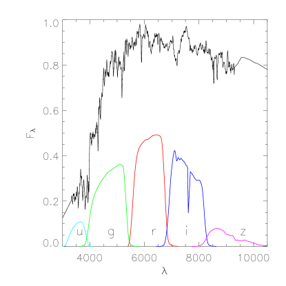
Figure 1: A model spectrum of an early type galaxy from Bruzual & Charlot (2003). The model was formed from a single burst of star formation 11 Gyr ago, and assumes a solar metallicity. Note the prominent break in the spectrum at 4000 Å. Also overplotted are the response functions (including atmospheric absorption) for the SDSS filters.

Unfortunately, as emphasized in Eisenstein et al. (2001), these simple colour cuts are not sufficient to select LRGs due to an accidental degeneracy in the SDSS filters that causes all galaxies, irrespective of type, to lie very close to the low redshift early type locus. We therefore follow the discussion there and impose a cut in absolute magnitude. We implement this by defining a colour to use as a proxy for redshift and then translating the absolute magnitude cut into a colour-magnitude cut. We see from Fig. 2 that $d_{\perp}$ correlates strongly with redshift and is appropriate to use for Cut II. For Cut I, we define,

$$c_{||}=0.7(g-r)+1.2(r-i-0.18)\,\,\,,$$ (6)

which is approximately parallel to the low redshift locus. Given these, we further impose

$${\rm Cut\,\,I:} r_{Petro}<13.6+c_{||}/0.3\,\,\,,$$ (7)

$$r_{Petro}<19.7\,\,\,;$$

$${\rm Cut\,\,II:} i<18.3+2d_{\perp}\,\,\,,$$ (8)

$$i<20\,\,\,.$$

Note we use $r_{Petro}$ for consistency with the SDSS LRG target selection. We note that Cut I is identical (except in the numerical values of the magnitude cuts in Eqs. 7) to the SDSS LRG Cut I, while the numerical values for Cut II were chosen to yield a population consistent with Cut I (see below). This was intentionally done to maximize the overlap between any sample selected using these cuts, and the SDSS LRG spectroscopic sample. The switch to the $i$ band for Cut II also requires some explanation. As is clear from Fig.1, the 4000 Å break is moving through the $r$ band throughout the fiducial redshift range of Cut II. This implies that the K-corrections to the $r$ band are very sensitive to redshift; the $i$ band K-corrections are much less sensitive to redshift allowing for a more robust selection.

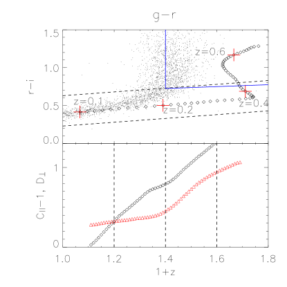
Figure 2: The top panel shows simulated $g-r$ and $r-i$ colours of an early-type galaxy as a function of redshift. The spectrum used to generate the track is the same as in Fig. 1, but evolved in redshift. Also shown are the colour cuts for Cut I (dashed, black) and Cut II galaxies (solid, blue). The points show the stellar locus as determined by a sample of stars with $r$-band magnitudes less than 19.5. The lower panel shows the colours $c_{||}$ (diamonds, black) and $d_{\perp}$ (triangles, red), as a function of redshift. Also shown are fiducial redshift boundaries for Cut I (0.2 – 0.4) and Cut II (0.4 – 0.6). Note that the range in $g-r$ is identical to the range in $1+z$.

The results of applying these cuts to the spectroscopic catalogs are shown in Fig. 3. Since the SDSS spectroscopic catalogue is at low redshift, we trim the catalogue using Cut I, while the higher redshift SDSS-2dF data are trimmed with Cut II. Our calibration dataset has 45,744 Cut I galaxies, and 1,474 Cut II galaxies. The large number of low redshift galaxies that pass Cut I indicate a failure of our selection criteria at redshifts lower than $z\sim 0.15$, as already noted by Eisenstein et al. (2001). We however leave these galaxies in our analysis, since they will contaminate any photometrically selected sample and it will be necessary to understand their photometric redshift distributions. No such problem exists for the Cut II galaxies, which have a negligible fraction of $z<0.4$ galaxies. The most significant contaminant for Cut II are M stars. The $g-r>1.4$ cut removes most of these, although there is a small residual level of contamination. Analyses using this or similar samples will have to estimate the effect of this contamination on their results.

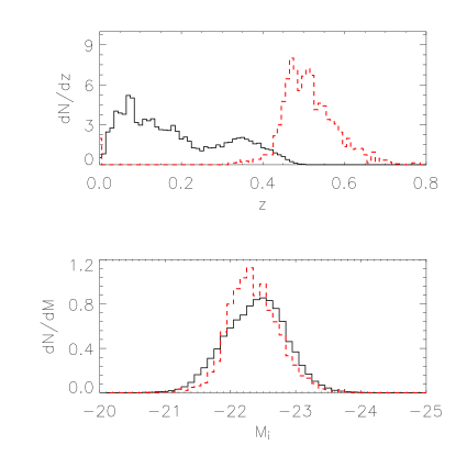
Figure 3: The top panel shows the spectroscopic redshift distribution, $dN/dz$ of the SDSS (solid, black) and the SDSS-2dF (dashed, red) samples trimmed using the selection criteria of Sec.2.3. Note that the SDSS sample is dominated by the low redshift MAIN sample, accounting for the low normalization at high redshift. The lower panel shows the $i$ band absolute magnitude distribution for the two samples, demonstrating that our absolute magnitude cuts are selecting a sample with $M_{i}\sim-22$ as desired. Both $dN/dz$ and $dN/dM$ are normalized so that they integrate to unity.

The lower panel of Fig. 3 shows the absolute magnitude distribution of both Cut I and Cut II galaxies. As expected, the colour magnitude cuts restrict the sample to bright galaxies; the median $i$ band magnitude is $M_{i}\sim-22$. Note that the Cut I and Cut II galaxies probe similar luminosities. The Cut I magnitude distribution also has a tail extending to low luminosities; this is the failure of the selection criteria at low redshift we encountered above.

3 Photometric Redshift Estimation

Photometric redshift estimation techniques can be classified into two groups, “empirical” and “template-fitting” methods. Empirical methods (Connolly et al., 1995; Brunner et al., 1999; Wang et al., 1998) are based on the observational fact that galaxies are restricted to a low dimensional surface in the space of their colours and redshift. Using a training set of galaxies, these methods attempt to parametrize this surface, either with low-order polynomials, nearest-neighbour searches or neural networks. The advantage of these methods is that they attempt to measure these relationships directly from the data, and so, implicitly correct for any calibration biases present. A publicly available example is the Artificial Neural Network code (Firth et al., 2003; Collister & Lahav, 2004, ANNz,) that trains a neural network to learn the relation between photometry and redshift from an appropriate training set of observed galaxies whose redshifts are already known. This code has a photometric redshift accuracy similar to the methods decribed below(Collister & Lahav, 2004).

The fact that these methods rely on training sets is their greatest disadvantage. For these methods to work, the training set must densely sample the entire redshift-colour space of interest, as it is difficult to extrapolate outside the domain of the training set. Most training sets, including the samples constructed above, violate the above requirement and therefore are of limited utility. Template-based methods do not suffer from these drawbacks, and form the basis for the two algorithms used in this paper, which we now discuss.

3.1 Simple Template Fitting

Template fitting methods start with a set of model spectra (the “templates”) of galaxies, either from spectrophotometrically calibrated observations of galaxies (Coleman et al., 1980) or from stellar synthesis models (Bruzual & Charlot, 2003; Le Borgne & Rocca-Volmerange, 2002). These methods then attempt to reconstruct the observed colours of galaxies by some (appropriately redshifted) linear combination of the templates, projected through the appropriate filters. The best fit redshift is then an estimate of the galaxy’s true redshift. Concretely, if we denote the templates by $\Psi^{i}(z)$, this algorithm can be cast as a minimization of

$$\chi^{2}(c_{i},z)=\sum_{\alpha}\left(\frac{f_{\alpha}-R_{\alpha}(\sum_{i}c_{i}\Psi^{i}(z))}{\sigma_{\alpha}}\right)^{2}\,\,\,,$$ (9)

where $f_{\alpha}$ is the observed flux (with error $\sigma_{\alpha}$) of the galaxy in the $\alpha$ filter, and $R_{\alpha}(\Psi)$ projects the spectrum $\Psi$ onto the $\alpha$ filter. For definiteness, we work with the AB photometric system (Oke & Gunn, 1983), where the apparent magnitude of a galaxy, $m_{AB}$, is related to its SED, $\Psi$ (with units of W m^-2 Hz^-1), by

$$m_{AB}=-2.5\log_{10}\left[\frac{\int\,d\nu\,\nu^{-1}\Psi(\nu)W_{\alpha}(\nu)}{\int\,d\nu\,\nu^{-1}g(\nu)W_{\alpha}(\nu)}\right]\,\,$$ (10)

where $W_{\alpha}$ is the response of the $\alpha$ filter. The reference SED is given by $g(\nu)=3631\rm{Jy}$ (where 1 Jy = $10^{-26}$ W m^-2 Hz^-1).

One of the advantages of the LRGs is that their spectra are well described by a single template (Eisenstein et al., 2003). We find that the LRG colours are well described by a Bruzual & Charlot (2003) single instantaneous burst template at solar metallicity with the burst occurring when the Universe was 2.5 Gyr old. The template evolves with time, becoming redder and increasing the 4000 Å break, as the more massive hot stars die. To incorporate this evolution, we interpolate between models with bursts with ages of [11, 5, 2.5, 1.4, 0.9, 0.64, 0.1] Gyr to calculate the template as a function of redshift. The photometric redshifts we derive are insensitive to the precise time of the burst, and therefore, we do not attempt any optimization of this parameter.

The implementation of this method we use is part of the IDLSPEC2D SDSS spectroscopic reduction pipeline (Burles & Schlegel, 2004) and can be downloaded through the WWW.

3.2 Hybrid Methods

Obviously, this simple template-fitting algorithm is effective only when the templates accurately describe the photometric properties of the galaxies for which one wants to estimate redshifts. This suggests generalizing the template-fitting algorithm by incorporating features of empirical methods (Csabai et al., 2000; Budavári et al., 2000, 2001). The basic approach is to divide a training set into spectral classes corresponding to each of the templates. Given these training sets for the individual templates, one can repair the templates by adjusting them to better reproduce the measured colours of the galaxies in the training set. By repeating this classification and repair procedure, one can obtain a improved template set that yields more reliable photometric redshifts (Csabai et al., 2003). Moreover, this process of adjusting the templates to agree with observations makes hybrid methods potentially less sensitive to potential systematic problems due to errors in the filter curves or photometric zeropoints. We refer the reader to the above papers for details on the implementation of this algorithm. For the LRGs, we start with an elliptical template from Coleman et al. (1980) and apply the above algorithm to optimize it. This is done in an iterative manner and converges after typically three iterations.

This single optimized template is used for an initial redshift estimate for all LRGs. The SDSS LRG sample is, however, selected assuming a passively evolving elliptical template (Eisenstein et al., 2001). Therefore, we expect to gain in photometric redshift accuracy if we allow the LRG spectral template to evolve with redshift. The SDSS and SDSS-2dF redshift samples are subdivided into three redshift intervals $0.00<z<0.35$, $0.25<z<0.45$ and $0.35<z<1.0$, based on the photometric redshifts of the individual galaxies. Within each interval we optimize the spectral template as described above. The overlapping redshift intervals provide a smooth progression in spectral type from one redshift interval to the next, as well as ensuring that the number and distribution of calibration redshifts is sufficient to constrain the colours of galaxies across a broad spectral range.

3.3 Results

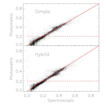
Figure 4: Scatter plot showing the photometric redshift versus the spectroscopic redshift for a random 10000 galaxies from our calibration sample. The upper panel shows the results for the simple template fitting code of Sec.3.1, and the lower panel are the results for the hybrid code of Sec.3.2. The solid (red) line has slope 1, while the dashed line marks the fiducial lower redshift limit of any photometric LRG sample. The difficulty of estimating redshifts at $z\sim 0.4$ is evident from the increased scatter.

We now apply the methods of the previous two sections to our calibration dataset; the results are summarized in Fig.4. Both are essentially unbiased ($|\Delta z_{mean}|<0.01$) at redshifts less that 0.5. At higher redshifts, the photometric redshifts are systematically lower than the spectroscopic redshifts by about 5%. The scatter in both methods is approximately $\sigma\sim 0.035$, except at redshifts greater than $0.55$, where the scatter grows to $\sim 0.06$, caused both by increased photometric scatter and increased uncertainties in templates (caused by for eg. star formation or emission lines).

There are two noticeable features in Fig.4 that deserve comment. The first is that the hybrid methods do significantly better than the single template fits at low redshifts ($z<0.15$). This is due to the failure of the LRG selection criteria at low redshifts; a single elliptical template no longer well describes this population. This highlights an important advantage of the hybrid methods – they adjust their templates to better describe the populations.

Figure 5: Simulations showing the effect of magnitude errors on the accuracy of the photometric redshifts. The upper left plot shows the reconstructed photometric redshifts for a magnitude error, $\sigma_{m}=0.03$ in all 5 bands, while the upper right panel has no S/N in the $u$ and $z$ bands and $\sigma_{m}=0.03$ in the remaining bands. The lower panel shows the redshift error induced by magnitude errors; the solid line has constant error across the bands, while the dashed line has constant error in $g,r,i$ and zero S/N in $u$ and $z$. Since the magnitude errors are independant of redshift, the redshift errors are simply computed over the entire redshift range.

The second feature is the increased scatter around $z\sim 0.4$, caused by an accidental degeneracy due to the SDSS filters. Fig. 1 shows a gap between the $g$ and $r$ bands at about 5500 Å. As the 4000 Å break enters this gap at $z\sim 0.38$, the lack of coverage in either the $g$ or $r$ band causes a degeneracy between the strength of the 4000 Å break and its location, increasing the redshift errors.

Figure 6: The double Gaussian fits to the error distribution as a function of spectroscopic redshift. The $x$ axis shows the redshift error, $z_{spectro}-z_{photo}$, and each panel is a redshift slice with the central redshift shown in the upper left. The histogram is the measured distribution, while the curves are the best fit Gaussian (both individually and summed). The data here are SDSS galaxies selected using Cut I. The photometric redshifts are estimated using the method of Sec. 3.2.

It is useful to be able to separate the effects of template errors from photometric errors in the redshift error budget. In order to do this, we simulate galaxies by uniformly distributing them between $0<z<0.8$ with synthetic colours given by the template used in the method of Sec.3.1. We then add errors to these synthetic fluxes; focussing on two extreme cases – uniform errors across all 5 bands, and no S/N in the $u$ and $z$ band (i.e. infinite magnitude errors corresponding to non-detection in $u$ and $z$ band, with uniform errors in the other bands). The latter case is motivated by the fact that the SDSS camera is least sensitive in the $u$ and $z$ bands, and because most LRGs are not detected in the $u$ band. The results of this exercise are shown in Fig. 5. The upper panels show a realization with a (optimistic) magnitude error, $\sigma_{m}\sim 0.03$. For comparison, the median S/N ($\sim 1/\sigma_{m}$) for LRGs at $z\sim 0.3$ is $\sim(2,30,70,80,30)$, and $\sim(0.5,10,25,36,15)$ at $z\sim 0.5$. A prominent feature is the degeneracy at $z\sim 0.4$ discussed above, for the case where the $u$ and $z$ bands have no signal. In this case, there is no extra information that can be used to break the degeneracy between the 4000 Å break strength and its location. Also, the scatter in the photometric redshifts increases for redshifts greater than $\sim 0.35$, coinciding with the 4000 Å break moving into the $r$ band, and the loss of redshift information from the $g-r$ colour. The lower panel shows how the redshift errors increase with increasing magnitude errors, again for the cases of uniform S/N in all bands, and in $g,r,i$ with zero S/N in $u$ and $z$. We also note that the redshift errors we measure are consistent with being caused principally by photometric scatter. However, the bias seen at high redshifts cannot be caused by photometric errors, and suggest either errors in the template, or errors in the photometric zeropoints or filter curves.

In order to parametrize the error distribution, we divide the calibration data into redshifts of width 0.05 (except between $z=0.6$ and $0.7$, which we combine because of the small number of galaxies in that range). Within each of these ranges, we fit the error distribution with a sum of Gaussians,

$$P(\delta z=z_{\rm spectro}-z_{photo})=\frac{1}{{\cal N}}\sum_{i=1}^{N}b_{i}\exp\left(\frac{-(\delta z-m_{i})^{2}}{2\sigma_{i}^{2}}\right)\,\,\,,$$ (11)

where ${\cal N}$ is the normalization given by

$${\cal N}=\sum_{i=1}^{N}\sqrt{2\pi}b_{i}\sigma_{i}\,\,\,.$$ (12)

We find, as shown in Figs. 6 and 7, that the error distribution is well approximated by two Gaussians. The parameters of the fits for both the simple template and hybrid methods are in Tables 3.3 and 3.3 respectively. We note that the cores of these error distributions are significantly tighter than the errors mentioned above. However, the error distributions typically have long wings that are responsible for most of the measured RMS errors. The discrepancies between the SDSS and SDSS-2dF samples in the overlap region are due to a colour bias introduced by the sharp colour cuts, resulting in a bias in the redshift estimation for Cut II galaxies between $z=0.35-0.45$. We therefore recommend using the SDSS distributions to $z=0.45$ for samples by combining Cut I and Cut II.

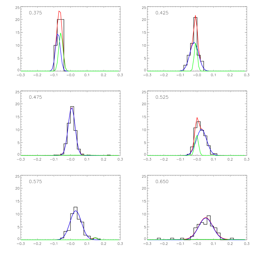
Figure 7: Same as Fig. 6 except for the SDSS-2dF galaxies selected using Cut II and from redshifts 0.35 to 0.7.

SDSS/SDSS-2dF Photometric redshift errors
Single Template Fitting
Double Gaussian fits
Catalogue	$z_{bin}$	$m_{1}$	$\sigma_{1}$	$m_{2}$	$\sigma_{2}$	$b$
SDSS	0.05-0.10	0.031	0.045	-0.194	0.084	0.002
SDSS	0.10-0.15	0.008	0.019	0.029	0.060	0.119
SDSS	0.15-0.20	0.010	0.015	0.013	0.052	0.059
SDSS	0.20-0.25	0.008	0.036	0.011	0.013	1.000
SDSS	0.25-0.30	0.002	0.018	-0.026	0.070	0.058
SDSS	0.30-0.35	-0.002	0.019	-0.030	0.040	0.338
SDSS	0.35-0.40	-0.004	0.028	0.000	0.000	1.000
SDSS	0.40-0.45	0.007	0.028	-0.003	0.014	1.000
SDSS	0.45-0.50	0.015	0.023	0.001	0.011	1.000
SDSS-2dF	0.35-0.40	-0.064	0.026	-0.069	0.002	1.000
SDSS-2dF	0.40-0.45	-0.019	0.022	-0.330	0.000	0.000
SDSS-2dF	0.45-0.50	0.003	0.030	0.010	0.016	1.000
SDSS-2dF	0.50-0.55	0.018	0.035	-0.278	0.000	0.000
SDSS-2dF	0.55-0.60	0.023	0.049	0.066	0.113	0.021
SDSS-2dF	0.60-0.70	0.039	0.047	0.011	0.093	0.423

Table 1: Double Gaussian fits to the photometric redshift error, $z-z_{p}$ as a function of $z$ for the SDSS and SDSS-2dF data. $(m_{1},\sigma_{1})$ and $(m_{2},\sigma_{2})$ are the mean and standard deviation of the first and second Gaussians respectively, while $b$ is the ratio of the amplitude of the second Gaussian to the first. The photometric redshifts were computed using the method of Sec.3.1. We recommend using the SDSS distributions to $z=0.45$ and SDSS-2dF for higher redshifts.

Table 2: Same as Table 3.3 except that the photometric redshifts were computed using the methods of Sec.3.2

In addition to measuring the error distribution, it is useful to measure the fraction of galaxies whose redshifts are “catastrophically” wrong. We define a catastrophic failure as a photometric redshift that differs from the spectroscopic redshift by more than $\Delta z_{c}$, where we use $\Delta z_{c}=0.1$ and $0.2$. For $\Delta z_{c}=0.1$, we have a catastrophic failure rate of 3.5% for the simple template fitting algorithm, and 1.5% for the hybrid algorithm. However, a large fraction of this is dominated by the underestimation of the photometric redshifts at $z>0.5$. If we increase $\Delta z_{c}$ to 0.2, the failure rate drops to under 0.5%.

4 Estimating $dN/dz\,$

In the previous section, we estimated the photometric redshift error distributions as a function of the true redshift of the galaxy. With this in hand, we turn to the problem of estimating the actual redshift distribution, $dN/dz\,$of a sample of galaxies given the distribution of their photometric redshifts, $[dN/dz]_{P}\,$.

As discussed in the Introduction, the apparently trivial solution to this problem is to measure the error distribution not as a function of the true redshift, but as a function of photometric redshift. One can then add these distributions, weighted by $[dN/dz]_{P}\,$to estimate the true redshift distribution. The problem with this approach is that the photometric redshift error distributions measured as a function of photometric redshift depend sensitively on the selection criteria of the calibration sample. If these criteria don’t match those of the full sample (and in general, they will not), then $dN/dz\,$estimated using the above technique will be biased.

In order to proceed, we observe that the photometric redshift distribution is simply the convolution of the true redshift distribution with redshift errors,

$$\left[\frac{dN}{dz}\right]_{P}\sim\left(\frac{dN}{dz}\right)\otimes\Delta z\,\,.$$ (13)

If we define $\Delta(z-z_{p},z)$ as the probability that a galaxy at redshift $z$ is scattered to photometric redshift $z_{p}$, then we can write out the above more concretely,

$$\left[\frac{dN}{dz}\right]_{P}(z_{p})=\int^{\infty}_{0}dz^{\prime}\,\left[\frac{dN}{dz}\right](z^{\prime})\Delta(z^{\prime}-z_{p},z^{\prime})\,\,,$$ (14)

where the left side has the known $[dN/dz]_{P}\,$, while the right is the unknown $dN/dz\,$. Eq. 14 is a Fredholm equation of the first kind and is ubiquitous throughout astronomy (Craig & Brown, 1986). Unfortunately, such problems do not possess a unique solution and moreover, are ill-conditioned. Small perturbations in the data can produce solutions that are arbitrarily different. This is not surprising, given that Eq.14 describes a smoothing operator that generically loses information, implying that the solution will in general require incorporating some “prior” knowledge about $dN/dz\,$.

4.1 Discretization and The Classical Solution

We begin by approximating $[dN/dz]_{P}\,$as a stepwise constant function measured in $n$ bins, $[z_{p}^{i},z_{p}^{i+1})$ with $i=0,\ldots n-1$, and $dN/dz\,$in $m$ bins, $[z^{j},z^{j+1})$ where $j=0,\ldots,m-1$. Substituting into Eq.14, we obtain

$$\left[\frac{dN}{dz}\right]_{P,i}=A_{ij}\left[\frac{dN}{dz}\right]_{j}$$ (15)

where we assume the Einstein summation convention. The response matrix $A_{ij}$ is given by

$$A_{ij}=\frac{1}{z_{p}^{i+1}-z_{p}^{i}}\int^{z_{p}^{i+1}}_{z_{p}^{i}}\,dz_{p}^{\prime}\int^{z^{j+1}}_{z^{j}}\,dz^{\prime}\Delta(z^{\prime}-z_{p}^{\prime},z^{\prime})\,\,.$$ (16)

For the specific case where $\Delta$ can be described by a sum of $N$ Gaussians (Eq. 11), one can do one of the integrals explicitly to obtain

$$A_{ij}=\frac{1}{z_{p}^{i+1}-z_{p}^{i}}\int^{z_{p}^{i+1}}_{z_{p}^{i}}\,dz_{p}^{\prime}\,\sqrt{\frac{\pi}{2}}\sum_{k=1}^{N}b_{k}\sigma_{k}\times$$

$$\left[f(\bar{z}_{k},z^{j+1},\sigma_{k},z_{p}^{\prime})-f(\bar{z}_{k},z^{j},\sigma_{k},z_{p}^{\prime})\right]\,\,,$$ (17)

where we define

$$f(\bar{z},z^{j},\sigma,z)={\rm erf}\left(\frac{|z^{j}-\bar{z}-z|}{\sqrt{2}\sigma}\right){\rm sgn}\left(\frac{z^{j}-\bar{z}-z}{\sqrt{2}\sigma}\right)\,\,\,.$$ (18)

where ${\rm sgn}$ is the sign operator and ${\rm erf}$ is the error function. Note that discretizing the problem has recast an integral equation (Eq.14) into a matrix problem (Eq. 15), albeit with a non-square matrix. We can obtain a solution to this problem by singular value decomposition (SVD, Press et al., 1992). We denote this the classical solution since we do not explicitly use any prior information about $dN/dz\,$.

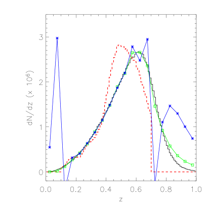
Figure 8: Results of simulations of the classical solution of the redshift inversion problem. The solid [black] histogram is the true redshift distribution, while the broken [red] histogram shows the photometric redshift distribution. The connected boxes [green] and stars [blue] show the reconstructed redshift distributions for different discretizations (10 and 15 bins, respectively) of the photometric redshift distributions. In both cases, the reconstructed distribution is parametrized by 20 step functions.

In order to understand the behaviour of the classical solution, we test it on simulations of the photometric redshift distribution. We start by distributing galaxies randomly in redshift between $z=0$ and $z=1$ according to,

$$\frac{dN}{dz}=\frac{z^{2}}{1+\exp(20z-14)}\,\,.$$ (19)

This distribution initially grows as $z^{2}$, and is exponentially cut off at $z\sim 0.6$, and approximates a volume limited distribution with a magnitude limit at high redshifts. Random redshift errors, using the model of Table 3.3, are added to obtain photometric redshifts, $z_{p}$. For redshifts greater than 0.7, the errors are sampled from a Gaussian whose mean and width are obtained by linearly extrapolating the errors from Table 3.3. Finally, we restrict to galaxies with $z_{p}\in[0.1,0.7]$. An example of the true and photometric redshift distributions is shown in Fig. 8.

The photometric redshift distribution is then discretized into $n$ bins, $[dN/dz]_{P,i}$. We present results for $n=10\,(\Delta z=0.06)$ and $n=15\,(\Delta z=0.04)$. The estimated $dN/dz$ is likewise parametrized as a piecewise constant function from $z=0$ to $z=1$ with a step width of $\Delta z=0.05$. Using these parametrizations, we construct the response matrix $A_{ij}$ (Eq.16) and solve for $dN/dz$ using Eq. 15. For the parameters considered here (and indeed, for generic choices), this is an underdetermined linear system. We solve it using SVD and backsubstitution (Press et al., 1992), setting singular values $<10^{-5}$ to zero. Fig. 8 shows the estimated $dN/dz$ averaged over 50 simulations, and compares it to the true redshift distribution.

The first observation is that the classical solution reconstructs the redshift distribution accurately for certain choices of discretizations, and in particular, for discretizations of the photometric distributions with step sizes approximately the width of the photometric redshift errors. The largest errors are for $z\geq 0.9$ that result from the fact that $dN/dz$ is almost completely unconstrained at these redshifts by $[dN/dz]_{P}$ as only 6 per cent of objects at these redshifts scatter to $z\leq 0.7$.

We also observe that as we increase the resolution of $[dN/dz]_{P}$, the reconstruction goes unstable, ringing at the edges of the photometric redshift catalogue. Note that the reconstructions in Fig. 8 are averages, and the instabilities in a single reconstruction are significantly larger.

This behaviour has a simple, intuitive explanation. The effect of photometric redshift errors is to smooth away the high frequency ((redshift error)^-1) components in $dN/dz$. However, $[dN/dz]_{P}$ has high frequencies due to noise in the data, and these induce large oscillations in the reconstruction. To be more quantitative, we start with a simplified model of the photometric errors,

$$\Delta(z-z_{p},z)\propto\exp\left(\frac{-(z-z_{p})^{2}}{2\sigma^{2}}\right)\,\,.$$ (20)

A component of $dN/dz$ with frequency $k$ will be attenuated by a factor of

$$\int dz\,\exp\left(\frac{-(z-z_{p})^{2}}{2\sigma^{2}}\right)e^{ikz}\propto\exp\left(-\frac{k^{2}\sigma^{2}}{2}\right)\,\,.$$ (21)

However, $[dN/dz]_{P}$ has a Poisson noise component that tends to a constant at high frequencies. Therefore, the inversion excites high frequency modes in the reconstruction with amplitude $\propto\exp(k^{2}\sigma^{2}/2)$. Eq. 21 also implies that this becomes significant for modes with $k>1/\sigma$, agreeing with our intuitive picture.

The effect of the discretization step size on the the stability of the classical solution is now clear; discretization cuts off frequencies higher than $\sim 1/\delta z$ where $\delta z$ is the step size, filtering out the problematic modes. This also suggests that the ideal discretizations have $\delta z\sim\sigma$, as demonstrated in our simulations.

4.2 Regularization

We would like to modify the classical solution so that it becomes less sensitive to the inversion instability discussed in the previous section. In order to do so, it is useful to rephrase the classical solution as a minimization problem. If we define the energy functional,

$$E_{0}=\left\arrowvert A_{ij}\left[\frac{dN}{dz}\right]_{j}-\left[\frac{dN}{dz}\right]_{P,i}\right\arrowvert^{2}\,\,,$$ (22)

then the classical solution is the value of $dN/dz$ that minimizes $E_{0}$. Given this description, it is trivial to include a penalty function that imposes smoothness on the reconstructed function,

$$E=E_{0}+\lambda P\,\,,$$ (23)

where $P$ is the penalty function and $\lambda$ adjusts the relative weight of $P$ in the minimization of $E$. There are number of possible choices for the $P$ that would impose smoothness; we use the forward difference operator,

$$P=\sum_{j=0}^{m-1}\left(\left[\frac{dN}{dz}\right]_{j+1}-\left[\frac{dN}{dz}\right]_{j}\right)^{2}\,\,\,.$$ (24)

There remains the problem of choosing an appropriate value for $\lambda$. Unfortunately, there is no a general method for choosing an optimal value. The best that we can do is to define a general merit function that objectively selects an appropriate range for $\lambda$. Based on the discussion in Craig & Brown (1986), we use

$$\Xi^{2}=\frac{1}{n}\sum_{i=0}^{n-1}\left[\left(A_{ij}\left[\frac{dN}{dz}\right]_{av,j}-\left[\frac{dN}{dz}\right]_{P,i}\right)\right]^{2}$$

$$+\frac{1}{m}\sum_{j=0}^{m-1}\left\langle\left(\left[\frac{dN}{dz}\right]_{j}-\left[\frac{dN}{dz}\right]_{av,j}\right)^{2}\right\rangle\,\,,$$ (25)

where the average reconstruction $[dN/dz]_{av,j}$ is estimated either from simulations or bootstrap resampling. The first term is a measure of how well the reconstructed $dN/dz$ reproduces the observed $[dN/dz]_{p}$; this term is minimized as $\lambda\rightarrow 0$ and increases with increasing $\lambda$. The second term, the error in the reconstruction, measures its stability to the presence of noise in the data. As $\lambda\rightarrow\infty$, the penalty function dominates the minimization and the reconstruction is the most stable. As $\lambda$ decreases, the reconstruction is more sensitive to noise in the data, increasing this term. Choosing a value of $\lambda$ near the minimum of $\Xi^{2}$ picks a compromise between an accurate and stable reconstruction.

Figure 9: The value of $\Xi^{2}$ as a function of $\lambda$ for the simulations discussed in the text. $\lambda$ has been rescaled such that $\lambda=1$ corresponds to equal weight being given to $E_{0}$ and $P$ in Eq. 23. The dotted and dashed lines show the error and stability components of Eq. 25 respectively. As expected, the error term increases with increasing $\lambda$, while the stability term decreases with increasing $\lambda$. The minimum of $\Xi^{2}$ occurs near $\lambda=0.5$.

In order to test this method, we return to the simulations of the previous section. Since the regularization removes the sensitivity to the discretization of the photometric distribution, we discretize $[dN/dz]_{P}$ into 50 bins of thickness $\Delta z=0.012$. The estimated redshift distribution is parametrized by 40 step functions of width $\Delta z=0.025$. Given these parameters, we must estimate the appropriate value of $\lambda$. To do this, we run 50 simulations for a given value of $\lambda$ to evaluate $\Xi^{2}$ and repeat this for a grid of values of $\lambda$. The results are shown in Fig. 9. We note that $\Xi^{2}$ has a well defined minimum, with the error and stability terms demonstrating the $\lambda$ dependence that we anticipated. Note that the error term does not go to zero as $\lambda\rightarrow 0$, but appears to asymptote to a non-zero constant. This is readily understood in terms of the discussion in the previous section : the measured $[dN/dz]_{P}$ has a high-frequency noise component that cannot be reproduced by the convolution of $dN/dz$ with the redshift errors. It is this noise component that is responsible for the non-zero value of the error term in $\Xi^{2}$ as $\lambda\rightarrow 0$.

The upper panel of Fig. 10 shows the average of 50 reconstructions of $dN/dz$ for values of $\lambda$ near the minimum of $\Xi^{2}$. We observe that for all the values of $\lambda$ considered in the figure, the reconstructions closely match the input redshift distribution for all redshifts $<0.7$. As before, the largest discrepancies are at high redshift because of the lack of constraint due to the upper photometric redshift limit of $0.7$. It is also instructive to consider extreme values of $\lambda$; these are shown in the lower panel of Fig.10. For small values of $\lambda$, the reconstructions are extremely noisy, while for large values of $\lambda$, the penalty function dominates the reconstruction. Note that the forward difference operator (Eq. 24) represents a constant prior, which is what we see the reconstructions approaching as $\lambda\rightarrow\infty$.

We make one cautionary observation. Based on Fig. 10, one might conclude that the best strategy for choosing $\lambda$ is to preferentially choose a smaller value than what is suggested by the minimum of $\Xi^{2}$. We however discourage this because, as indicated in Fig.9, such reconstructions are very noisy. This lack of stability would result in small errors in the redshift error distribution being amplified in the reconstructions.

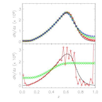
Figure 10: Regularized estimates of $dN/dz$ for different values of the regularization parameter, $\lambda$. In both panels, the black histogram shows the true redshift distribution. The upper panel shows the reconstructions for values of $\lambda$ about the minimum of $\Xi^{2}$; the stars (red), diamonds (green), and crosses (blue) correspond to $\lambda=0.1,0.5,$ and $1.0$ respectively. The lower panel shows the reconstructions for extreme values of $\lambda$, the crosses (red) and diamonds (green) correspond to $\lambda=10^{-10}$ and $1000$ respectively. The values of $\lambda$ have been rescaled as in Fig. 9.

How many galaxies are required for the inversion? The simulations discussed above used 100,000 galaxies, similar to the expected number of photometric LRGs over the same area of sky. We have however tested the inversion on as few as 1000 galaxies, and found that, for appropriate regularizations, the algorithm reconstructs the input redshift distribution. However, for small samples, the Poisson noise in the input photometric redshift distribution can be significant, resulting in a noisier reconstruction (for the same redshift resolution). This may be improved by smoothing the resulting reconstruction or equivalently, reconstructing the redshift distribution on a coarser redshift grid.

There is an important generalization of this method that should be mentioned. We introduced the concept of regularization and the penalty function to cure an instability in the deconvolution as we attempted a finer resolution of the redshift distribution. Phrased differently, the deconvolution became unstable when when the input became low S/N and the prior (in the form of the penalty function) compensated for this loss of information. In the cases considered in this paper, we have used a relatively weak prior; however, if one has reliable prior information (for eg. the rough shape of the redshift distribution), one can easily include that information. A strong prior will allow one to obtain a solution even in the low S/N regime. We do however remind the overzealous reader that the usual caveat about strong priors does apply in the case; the method cannot distinguish an incorrect prior, and will get the wrong answer if such a prior is heavily weighted.

4.3 Application to SDSS Data

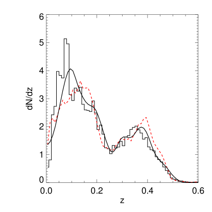
Figure 11: Regularized estimate [solid, black] of $dN/dz$ for the Cut I calibration data [histogram]. The input photometric redshift distribution is the dashed [red] line. $dN/dz$ is normalized to integrate to unity.

Before applying this algorithm to a photometric sample, we test it against the Cut I calibration dataset described in Sec.2.3. The results are in Fig.11. The reconstructed redshift distribution correctly captures all the broad features of the true redshift distribution, including correcting for the bias at $z\sim 0.1$ and sharpening the dip at $z\sim 0.25$. Fig.11 also highlights the inability of this method to reconstruct sharp features since these are disfavoured by the smoothness prior we impose; the inversion works best for broad features. It is worth emphasizing that most sharp features (including the feature at $z\sim 0.075$) are spurious (eg. binning artifacts). However, if a sharp feature is physically expected in the distribution, the prior must be adjusted to allow for this.

We conclude this discussion by applying the above algorithm to the SDSS photometric data. A detailed discussion of the construction and properties of the SDSS photometric LRG sample will be presented elsewhere; briefly, the sample is constructed by applying the photometric selection criteria (Cut I and Cut II, see Sec. 2.3) to objects classified as galaxies by the photometric pipeline. We then estimate a photometric redshift for each of the selected objects using the simple template fitting code of Sec. 3.1; however, the results are insensitive to the choice of algorithm. The photometric redshift distribution is shown in Fig. 12.

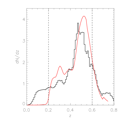
Figure 12: Regularized estimate [solid, red] of $dN/dz$ for the LRG sample culled from the SDSS photometric data, compared with the photometric redshift distribution [histogram, black]. The redshift distribution is for galaxies with $0.2<z_{photo}<0.6$, indicated by the vertical dashed lines. As before, $dN/dz$ is normalized to integrate to unity.

One feature of this distribution that deserves some explanation is the “bump” in the number of galaxies at $z\sim 0.7$. This is inconsistent with being the same population of LRGs selected with an apparent magnitude cut. It is unlikely that these are a different population at $z\sim 0.7$, as they would have to be a significantly brighter population than the LRGs, that only appeared at high redshifts. A more likely explanation is that these are faint galaxies at lower redshifts scattered to high redshifts by photometric errors. This is more likely, in light of the fact that these galaxies have $i\sim 20,g-r\sim 2$ and $r-i\sim 1$, giving them $r\sim 21$ and $g\sim 23$. This is at the very edge (or beyond) the photometric completeness of SDSS, and the measurements will have significant photometric errors ($\sim$ tenths of a magnitude). Given such photometric errors, it is likely for the more numerous low redshift galaxies to be scattered into the LRG colour space. Furthermore, the spectral templates that we use are not well constrained by observations for redshifts $>0.7$. To avoid the complications of correcting for such contamination, we restrict our catalog to $z_{photo}<0.6$. Similarly, as discussed earlier, the photometric selection breaks down at low redshifts, and so, we impose a lower redshift cutoff of $z_{photo}>0.2$. Note that this lower redshift cut is imposed only to select a uniform sample; the inversion must be (and is) performed at all redshifts. However, the small photometric redshift error at these redshifts minimizes the contamination from these galaxies, effectively truncating the inverted distribution at $z\sim 0.2$.

We can now apply the inversion algorithm to estimate the true redshift distribution, using the error distributions measured in Sec. 3.3. The merit function, Eq.25, is computed by bootstrap resampling the actual catalog; the measured $\Xi^{2}$ has a form similar to Fig. 9. Using the value of the regularization parameter, $\lambda$, obtained from $\Xi^{2}$, we show the estimated redshift distribution for galaxies with $0.2<z_{photo}<0.6$ in Fig. 12. The underestimation of the photometric redshifts at high redshifts is immediately apparent from the comparison of the two distributions. The bumps from $z=0.3$ to $0.4$ are a residual artifact of the inversion. These vanish for higher values of $\lambda$, and become stronger for lower regularizations, but are more unstable. The value of $\lambda$ used is a balance between this stability and accuracy, as intended.

5 Discussion

As we discussed in the Introduction, constructing a photometric redshift catalogue involves three steps – photometrically selecting a sample for which accurate photometric redshifts can be obtained, measuring the photometric redshift error distribution for the resulting sample, and estimating the true redshift distribution. This paper describes all stages of this process.

• We describe the selection of a sample of Luminous Red Galaxies (LRGs) using the SDSS photometric sample. These galaxies are typically old elliptical systems with strong 4000 Åbreaks in their continua. The shifting of this feature through the SDSS filters make accurate photometric redshifts possible.

• We measure the error distribution of this sample by comparing photometric and spectroscopic redshifts for a calibration subsample of galaxies culled from the SDSS and SDSS-2dF spectroscopic catalogues. The scatter in the redshifts is approximately $\sigma\sim 0.03$ at redshifts less than 0.55, and increases at higher redshifts due to increased photometric errors and uncertainties in the templates.

• The accuracy of the photometric redshifts is similar for the two algorithms we consider, a simple template fit and a hybrid algorithm that adjusts the template to better fit the observed colour distribution.

We have specifically used the SDSS photometric sample throughout this paper, both as a example and for its intrinsic interest. However, we emphasize that the entire process that we describe can be reconstructed for any multi-colour imaging survey with appropriate filters.

Using such a photometric redshift sample requires knowing the conditional probability that a galaxy with a photometric redshift, $z_{photo}$ has a true redshift, $z_{spectro}$. Given the redshift error distribution, this conditional probability can be readily estimated using Bayes’ theorem if the true underlying redshift distribution is known. Using the fact that the photometric redshift distribution is the true redshift distribution convolved with redshift errors, we have presented a method to deconvolve the errors to estimate the redshift distribution. This method is ill-conditioned, and therefore, we use a prior on the smoothness of the redshift distribution to regularize the deconvolution. We have calibrated the relative weight of this prior by measuring the accuracy and stability of the recovered redshift distributions, and we proposed a general merit function that objectively determines this weight.

We conclude with a few comments about this algorithm.

• The particulars of the sample selection are encoded into the photometric error distribution. The method is therefore completely general, and applicable to any combination of colour selections and photometric redshift cuts.

• The accuracy of the recovered redshift distribution is determined by the accuracy of the input error distributions. Therefore, it is essential that the calibration data used to measure the error distribution correspond as closely as possible to the actual data, both in photometric depth and accuracy. One can attempt to extrapolate these distributions to fainter magnitudes or measure them from simulations, but with the caveat that the actual distributions may be very different from these, and that the reconstruction could potentially be sensitive to these errors. We emphasize that this limitation is not unique to this methods, but affects all analyses that use photometric redshifts.

• The deconvolution algorithm is formally applicable to arbitrary error distributions. However, for complex error distributions (eg. multiply peaked distributions), multiple solutions may exist and there is no guarantee that the method will converge to the correct solution. This problem is avoided here by the use of photometric pre-selection; in general, it could also be prevented by the use of priors in the photometric redshift estimation. We strongly recommend using one of these methods to break photometric redshift degeneracies.

• An advantage to this method is that the calibration data need not sample the redshift range of interest in the same manner as the photometric data. It suffices that it samples the entire range well enough to measure the error distributions. This allows the use of calibration sets from heterogeneous samples, as was done in this paper.

• The inversion algorithm presented in this paper presents an alternative to iterative deconvolution algorithms (Lucy, 1974; Brodwin et al., 2003). As emphasized by Lucy (1974), the two methods have very different mathematical philosophies; iterative methods treat the problem as one in statistical estimation, while the philosophy in this paper derives from the theory of integral equations. However, in the high S/N regime, both methods will produce similar results, and there is little to distinguish the two. For low S/N, the deconvolution problem may not possess a solution, and iterative methods may not converge. In these cases, the algorithm presented in this paper transparently allows the inclusion of external information as part of the penalty function to yield a meaningful solution. In cases where one possesses reliable prior information, one can then refine that information to yield a better solution.

N.P. acknowledges useful discussions with Michael Blanton, Chris Hirata, Doug Finkbeiner, Jim Gunn, David Hogg and Željko Ivezić on photometric redshift estimation techniques and regularization methods. We thank the referee for a careful reading and suggesting a number of improvements, from which the paper has benefited.

Funding for the creation and distribution of the SDSS Archive has been provided by the Alfred P. Sloan Foundation, the Participating Institutions, the National Aeronautics and Space Administration, the National Science Foundation, the U.S. Department of Energy, the Japanese Monbukagakusho, and the Max Planck Society. The SDSS Web site is http://www.sdss.org/.

The SDSS is managed by the Astrophysical Research Consortium (ARC) for the Participating Institutions. The Participating Institutions are The University of Chicago, Fermilab, the Institute for Advanced Study, the Japan Participation Group, The Johns Hopkins University, Los Alamos National Laboratory, the Max-Planck-Institute for Astronomy (MPIA), the Max-Planck-Institute for Astrophysics (MPA), New Mexico State University, University of Pittsburgh, Princeton University, the United States Naval Observatory, and the University of Washington.

The SDSS-2dF Redshift Survey was made possible through the dedicated efforts of the staff at the Anglo-Australian Observatory, both in creating the 2dF instrument and supporting it on the telescope.

References

- Abazajian et al. (2004) Abazajian K. et al., 2004, AJ, 128, 502
- Abazajian et al. (2003) Abazajian K. et al., 2003, AJ, 126, 2081
- Benítez (2000) Benítez N., 2000, ApJ, 536, 571
- Blanton et al. (2003) Blanton M. R., Lin H., Lupton R. H., Maley F. M., Young N., Zehavi I., Loveday J., 2003, AJ, 125, 2276
- Bolzonella et al. (2000) Bolzonella M., Miralles J.-M., Pelló R., 2000, A&A, 363, 476
- Brodwin et al. (2003) Brodwin M., Lilly S. J., Porciani C., McCracken H. J., Fevre O. L., Foucaud S., Crampton D., Mellier Y., 2003, astro-ph/0310038
- Brunner et al. (1999) Brunner R. J., Connolly A. J., Szalay A. S., 1999, ApJ, 516, 563
- Bruzual & Charlot (2003) Bruzual G., Charlot S., 2003, MNRAS, 344, 1000
- Budavári et al. (2003) Budavári T. et al., 2003, ApJ, 595, 59
- Budavári et al. (2000) Budavári T., Szalay A. S., Connolly A. J., Csabai I., Dickinson M., 2000, AJ, 120, 1588
- Budavári et al. (2001) Budavári T., Szalay A. S., Csabai I., Connolly A. J., Tsvetanov Z., 2001, AJ, 121, 3266
- Burles & Schlegel (2004) Burles S., Schlegel D. J., 2004, in preparation
- Cannon et al. (2003) Cannon R., Croom S., Pimbblet K., for the SDSS-2dF Team , 2003, AAO Newsletter, 103, 8
- Coleman et al. (1980) Coleman G. D., Wu C.-C., Weedman D. W., 1980, ApJS, 43, 393
- Collister & Lahav (2004) Collister A. A., Lahav O., 2004, PASP, 116, 345
- Connolly et al. (1995) Connolly A. J., Csabai I., Szalay A. S., Koo D. C., Kron R. G., Munn J. A., 1995, AJ, 110, 2655
- Craig & Brown (1986) Craig I. J. D., Brown J. C., 1986, Inverse problems in astronomy: A guide to inversion strategies for remotely sensed data. Adam Hilger, Ltd., 1986, 159 p.
- Csabai et al. (2003) Csabai I., Budavári T., Connolly A. J., et al , 2003, AJ, 125, 580
- Csabai et al. (2000) Csabai I., Connolly A. J., Szalay A. S., Budavári T., 2000, AJ, 119, 69
- Eisenstein et al. (2001) Eisenstein D. J. et al., 2001, AJ, 122, 2267
- Eisenstein et al. (2003) Eisenstein D. J. et al., 2003, ApJ, 585, 694
- Firth et al. (2003) Firth A. E., Lahav O., Somerville R. S., 2003, MNRAS, 339, 1195
- Fukugita et al. (1996) Fukugita M., Ichikawa T., Gunn J. E., Doi M., Shimasaku K., Schneider D. P., 1996, AJ, 111, 1748
- Gladders & Yee (2000) Gladders M. D., Yee H. K. C., 2000, AJ, 120, 2148
- Gunn et al. (1998) Gunn J. E. et al., 1998, AJ, 116, 3040
- Gwyn & Hartwick (1996) Gwyn S. D. J., Hartwick F. D. A., 1996, ApJ, 468, L77
- Hamilton (1985) Hamilton D., 1985, ApJ, 297, 371
- Hogg et al. (1998) Hogg D. W., Cohen J. G., Blandford R., Gwyn S. D. J., et al , 1998, AJ, 115, 1418
- Hogg et al. (2001) Hogg D. W., Finkbeiner D. P., Schlegel D. J., Gunn J. E., 2001, AJ, 122, 2129
- Koo (1985) Koo D. C., 1985, AJ, 90, 418
- Le Borgne & Rocca-Volmerange (2002) Le Borgne D., Rocca-Volmerange B., 2002, A&A, 386, 446
- Lewis et al. (2002) Lewis I. J. et al., 2002, MNRAS, 333, 279
- Lucy (1974) Lucy L. B., 1974, AJ, 79, 745
- Lupton (2004) Lupton R. H., 2004, in preparation
- Nichol (2003) Nichol R. C., 2003, Carnegie Observatories Astrophysics Series, Vol. 3, ed. J. S. Mulchaey, A. Dressler, and A. Oemler (Cambridge: Cambridge Univ. Press)
- Oke & Gunn (1983) Oke J. B., Gunn J. E., 1983, ApJ, 266, 713
- Pier et al. (2003) Pier J. R., Munn J. A., Hindsley R. B., Hennessy G. S., Kent S. M., Lupton R. H., Ivezić Ž., 2003, AJ, 125, 1559
- Press et al. (1992) Press W. H., Teukolsky S. A., Vetterling W. T., Flannery B. P., 1992, Numerical recipes in FORTRAN. The art of scientific computing. Cambridge University Press, 1992, 2nd ed.
- Sawicki et al. (1997) Sawicki M. J., Lin H., Yee H. K. C., 1997, AJ, 113, 1
- Schneider et al. (1983) Schneider D. P., Gunn J. E., Hoessel J. G., 1983, ApJ, 264, 337
- Smith et al. (2002) Smith J. A. et al., 2002, AJ, 123, 2121
- Stoughton et al. (2002) Stoughton C., Lupton R. H., Bernardi M., Blanton M. R., et al , 2002, AJ, 123, 485
- Strauss et al. (2002) Strauss M. A. et al., 2002, AJ, 124, 1810
- Wang et al. (1998) Wang Y., Bahcall N., Turner E. L., 1998, AJ, 116, 2081
- Willis et al. (2001) Willis J. P., Hewett P. C., Warren S. J., 2001, MNRAS, 325, 1002
- York et al. (2000) York D. G. et al., 2000, AJ, 120, 1579