Power Spectrum Tomography with Weak Lensing

Abstract

Upcoming weak lensing surveys on wide fields will provide the opportunity to reconstruct the structure along the line of sight tomographically by employing photometric redshift information about the source distribution. We define power-spectrum statistics, including cross correlation between redshift bins, quantify the improvement that redshift information can make in cosmological parameter estimation, and discuss ways to optimize the redshift binning. We find that within the adiabatic cold dark matter class of models, crude tomography using two or three redshift bins is sufficient to extract most of the information and improve the measurements of cosmological parameters that determine the growth rate of structure by up to an order of magnitude.

1. Introduction

With new instruments such as MEGACAM at CFHT (Boulade et al.  1998) and the VST at the European Southern Observatory (Arnaboldi et al.  1998), wide-field surveys detect the weak lensing of faint galaxies by large scale structure will soon become a reality (see Melier  1998 for a recent review). Weak lensing by large-scale structure produces a correlated distortion in the ellipticities of the galaxies on the percent level (Blandford et al. 1991; Miralda-Escude  1991; Kaiser 1992) which can be used to measure a two-dimensional projection of the intervening mass distribution (Tyson, Valdes & Wenk 1990; Kaiser & Squires 1993).

If the redshift of the source galaxies are known, then more information can be extracted out of weak lensing by tomography, i.e. differencing the two-dimensional projected images to recover the three-dimensional distribution. In the absence of spectroscopy, approximate redshifts for the faint galaxies can be determined through photometric techniques (see e.g. Hogg et al. 1998 and references therein) and with the large number of galaxies at $R\lesssim 25$ ($\sim 10^{5}$ deg^-2) the properties of distribution can be known to good accuracy (Seljak 1998). Indeed the weak lensing surveys already plan to use photometric redshift information at least on a small subsample to measure the low order moments of the distribution such as its mean. These are important for determining the cosmological implications of the data (Smail et al. 1995; Fort et al. 1995; Luppino & Kaiser 1997).

The potential of tomographic techniques, especially in the wide-field limit where the cosmological information is completely contained in the two-point functions or power spectra, remains largely unexplored. Indeed most studies of weak lensing (e.g. Jain & Seljak 1997; Kaiser 1998; Hu & Tegmark 1999) simply assume a delta-function distribution of galaxies making tomography impossible.

In this Letter, we study the prospects for weak lensing tomography within the framework of the adiabatic cold dark matter (CDM) class of models for structure formation. We begin by defining the power spectrum statistics for an arbitrary set of galaxy redshift distributions. These are the power spectrum of the convergence map for each distribution and the cross-correlation between the maps. We then quantify how much additional information can be extracted by subdividing a single magnitude-limited sample into bins in redshift and analyzing their joint power spectra and cross-correlation. We conclude with a discussion of how errors in photometric redshifts might affect tomographic techniques.

2. Power Spectra

Generalizing the results of Kaiser (1992, 1998), we define the angular power spectra and cross-correlation of sky maps of the convergence based on a series of galaxy redshift distributions $n_{i}(z)$ (see also Seljak 1998)

$${{\bf P}^{\kappa}_{ij}}(\ell) \equiv {1\over 2\ell+1}\left<a^{*}_{(\ell m)\,i}a_{(\ell m)\,j}\right>\,$$ (1)

$$\approx 2\pi^{2}\ell\int dD\,{{g_{i}(D)g_{j}(D)}\over D_{A}^{3}(D)}\Delta_{\Phi}^{2}(k_{\ell},D)\,,$$

where $a_{(\ell m)\,i}$ are the spherical harmonic coefficients of the maps. Here $D=\int_{0}^{z}(H_{0}/H)dz$ is the dimensionless comoving distance and

$$D_{A}(D)=\Omega_{K}^{-1/2}{\sinh(\Omega_{K}^{1/2}D)}$$ (2)

is the dimensionless angular diameter distance, where $\Omega_{K}=1-\sum_{i}\Omega_{i}$ is the effective density in spatial curvature in units of the critical density. The efficiency with which gravitational potential fluctuations $\Phi$, as measured by their dimensionless power per logarithmic interval $\Delta_{\Phi}^{2}\equiv k^{3}P_{\Phi}/2\pi^{2}$, lens the given galaxy distribution $n_{i}$ is described by

$$g_{i}(D)=D_{A}(D)\int_{D}^{\infty}dD^{\prime}\,\left[n_{i}{{dz\over dD}}\right](D^{\prime}){D_{A}(D^{\prime}-D)\over D_{A}(D^{\prime})}\,.$$ (3)

Note that $n_{i}$ is normalized so that $\int_{0}^{\infty}dz\,n_{i}(z)=1$. Finally $k_{\ell}=\ell H_{0}/D_{A}(D)$ is the wavenumber which projects onto the angular scale $\ell$ at distance $D$. For small fields of view, the spherical harmonics of order $\ell$ can be replaced by Fourier modes with angular frequency $\omega$.

We use the Peacock & Dodds (1996) scaling relations to evalute $\Delta_{\Phi}^{2}$ in the non-linear density regime. Equation (1) assumes that the redshift distributions are sufficiently wide to encompass many wavelengths of the relevant fluctuations ($2\pi/k_{\ell}$) along the line of sight so that the Limber equation holds even tomographically (see Kaiser 1998).

These power spectra define the cosmic signal. Shot noise in the measurement from the intrinsic ellipticity of the galaxies adds white noise to the cosmic signal making the observed power spectra

$${\bf C}_{ij}(\ell)={{\bf P}^{\kappa}_{ij}}(\ell)+{\left<\gamma_{\rm int}^{2}\right>\delta_{ij}/\bar{n}_{i}}\,,$$ (4)

where $\left<\gamma_{\rm int}^{2}\right>^{1/2}$ is the rms intrinsic shear in each component, and ${\bar{n}}_{i}$ is the number density of the galaxies per steradian on the sky in the whole distribution $n_{i}(z)$.

Figure 1.— Subdividing the source population. Partitioning the galaxies by the median redshift (or distance $D$) yields lensing efficiencies with strong overlap.

The distributions $n_{i}(z)$ need not be physically distinct galaxy populations. Consider a total distribution $n(z)$ with

$$\left[n{dz\over dD}\right](D)\propto D^{\alpha}\exp[-(D/D_{*})^{\beta}]\,,$$ (5)

which roughly approximates that of a magnitude-limited survey, and take $\alpha=1,\beta=4$ for definiteness (assumed throughout unless otherwise stated). One can subdivide the sample into redshift bins to define the distributions $n_{i}(z)$. The power spectra for cruder partitions can always be constructed out of finer ones: if the $j$ and $k$ bins are combined, then

$$\bar{n}_{j+k}^{2}{\bf P}_{(j+k)(j+k)}^{\kappa} = \bar{n}_{j}^{2}{\bf P}_{jj}^{\kappa}+2\bar{n}_{j}\bar{n}_{k}{\bf P}_{jk}^{\kappa}+\bar{n}_{k}^{2}{\bf P}_{kk}^{\kappa}\,,$$

$$\bar{n}_{j+k}{\bf P}_{i(j+k)}^{\kappa} = \bar{n}_{j}{\bf P}_{ij}^{\kappa}+\bar{n}_{k}{\bf P}_{ik}^{\kappa}\,.$$ (6)

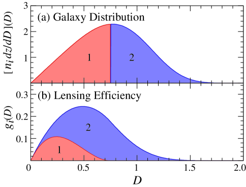
In Fig. 1, we show an example where the galaxies with $z<z_{\rm median}$ are binned into $n_{1}$ and the rest into $n_{2}$. Here and throughout we will take our fiducial cosmology as an adiabatic CDM model with matter density $\Omega_{m}=0.35$, dimensionless Hubble constant $h=0.65$, baryon density $\Omega_{b}=0.05$, cosmological constant $\Omega_{\Lambda}=0.65$, neutrino mass $m_{\nu}=0.7$ eV, the initial potential power spectrum amplitude $A$, and tilt $n_{S}=1$.

We also plot in Fig. 1 the lensing efficiency function $g_{i}(D)$. Notice that despite having non-overlapping source distributions (upper panel), the lensing efficiencies strongly overlap (bottom panel) implying that the resulting convergence maps will have a correspondingly large cross correlation. This is of course because the high and low redshift galaxies alike are lensed by low-redshift structures. Also for this reason, there will be always be a stronger signal in the high redshift bins. This fact will be important for signal-to-noise considerations in choosing the bins.

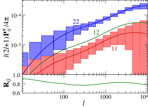
All of these properties can be seen in Fig. 2, where we plot the resultant power spectra and their cross correlation for the equal binning of Fig. 1.

Figure 2.— Power spectra and cross correlation for a subdivision in two across the median redshift $z_{\rm median}=1$ and errors for a survey of $5^{\circ}$ on the side, $\left<\gamma_{\rm int}^{2}\right>^{1/2}=0.4$, and $\bar{n}=2\times 10^{5}$ deg^-2. Note the strong correlation ${\bf R}_{ij}$ between the two power spectra make the combination of the power spectra less constraining than a naive interpretation of the individual errors would imply.

3. Redshift Binning and Parameter Estimation

While subdividing the sample into finer bins always increases the amount of information, there are two considerations that limit the effectiveness of redshift divisions. The first is set by the shot noise from the intrinsic ellipticities of the galaxies. Once the number density $\bar{n}_{i}$ per bin is so small that shot noise surpasses the signal in equation (4), further subdivision no longer helps. The point at which this occurs depends on the angular scale of interest. The greater number of galaxies encompassed by the larger angular scales boosts the signal to noise (see Fig. 2 and Kaiser 1992). Based on this criterion, one should separately subdivide the data to extract the maximal large and small angle information.

However there is a second consideration. If the lensing signal does not change significantly across the redshift range of the whole distribution, then subdivision will not add information. These considerations can be quantified by considering the correlation coefficient between the power spectra of the subdivisions: ${\bf R}_{ij}={\bf P}^{\kappa}_{ij}/({\bf P}^{\kappa}_{ii}{\bf P}^{\kappa}_{jj})^{1/2}$. For the model of Fig. 2, the power spectra are highly correlated (${\bf R}_{12}\sim 0.8$) even with only two subdivisions. Thus even though there is enough signal to noise to subdivide the sample further, one gains little information by doing so.

One can combine these two considerations by diagonalizing the covariance matrix and considering the signal to noise in the diagonal basis. The appropriate strategy for subdivision depends on the true redshift distribution of the galaxies and the model for structure formation. One should therefore perform this test on the actual data to decide how to subdivide the sample.

Nevertheless, to make these considerations more concrete, let us consider the specific goal of measuring the cosmological parameters $p_{\alpha}$ assuming that the underlying adiabatic CDM cosmology described above is correct. The Fisher information matrix can be used to quantify the effect of subdivision. It is defined as

$${\bf F}_{\alpha\beta}=-\left<\partial^{2}\ln L\over\partial p_{\alpha}\partial p_{\beta}\right>_{\bf x}\,,$$ (7)

where $L$ is the likelihood of observing a data set ${\bf x}$ given the true parameters $p_{1}\ldots p_{\alpha}$.

Generalizing the results of Hu & Tegmark (1998) to multiple correlated power spectra, we obtain

$${\bf F}_{\alpha\beta}=\sum_{\ell=2}^{\ell_{\rm max}}({\ell+1/2})f_{\rm sky}{\rm tr}[{\bf C}^{-1}{\bf C}_{,\alpha}{\bf C}^{-1}{\bf C}_{,\beta}]\,,$$ (8)

under the assumption of Gaussian signal and noise, where $f_{\rm sky}$ is fraction of sky covered by the survey, the covariance matrix ${\bf C}$ was defined in equation (4), and commas denote partial derivatives with respect to the cosmological parameters $p_{\alpha}$. We take $\ell_{\rm max}=3000$ to approximate the increased covariance due to the nonlinearities producing non-Gaussianity in the signal (Scoccimarro, Zaldarriaga & Hui 1999). Since the variance of an unbiased estimator of a parameter $p_{\alpha}$ cannot be less than $\sigma(p_{\alpha})=({\bf F}^{-1})_{\alpha\alpha}$, the Fisher matrix quantifies the best statistical errors on parameters possible with a given data set.

For the purposes of this work, the absolute errors on parameters are less relevant than the improvement in errors from subdividing the data (see Hu & Tegmark for the former). We therefore test a 4 dimensional subset of the adiabatic CDM parameter space to see how subdivision can help separate initial power ($A$) from the various contributors to the redshift-dependent evolution of power ($\Omega_{\Lambda}$,$\Omega_{K}$,$m_{\nu}$). For reference the standard errors $\sigma_{\alpha}$ for this parameter space without subdivision are given in Table 1. Errors in the full parameter space would be increased but note that the neglected parameters $(\Omega_{m}h^{2}$,$\Omega_{b}h^{2}$, and $n_{S}$) are exactly those that the CMB satellite experiments should constrain precisely (see e.g. Jungman et al. 1996; Eisenstein et al. 1999).

As an example, we take a sample with $z_{\rm median}=1$ and $\bar{n}=2\times 10^{5}$ deg^-2 as appropriate for a magnitude limit of $R\sim 25$ (see Smail et al. 1995b). The signal to noise in the full sample is quite high, e.g. at $\ell=100$, $S/N\sim 25$. Thus we expect that subdividing the sample should improve parameter estimation.

TABLE 1

Parameter Estimation for $z_{\rm median}=1$

$p_{\alpha}$	$\sigma_{\alpha}f_{\rm sky}^{1/2}$	Error Improvement
	1	2(${1\over 2}$)	2(${1\over 4}$)	2(${1\over 8}$)	3(${1\over 3}$)	3(${1\over 4}$)	3(${1\over 8}$) [
$\Omega_{\Lambda}$	0.040	6.5	6.9	5.7	7.2	7.7	6.9
$\Omega_{K}$	0.023	2.9	3.1	2.9	3.3	3.5	3.2
$m_{\nu}$	0.044	1.7	2.0	2.1	2.1	2.2	2.2
$\ln A$	0.064	1.7	2.0	2.0	2.1	2.2	2.1

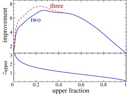
As shown in Table 1, subdividing this sample in equal halves, denoted as 2(1/2), improves the errors $\sigma_{\alpha}$ by a factor of 2 to 7. Since the signal in the lower redshift bin is smaller than in the higher redshift bin, it suffers comparatively more from the intrinsic noise variance. One can optimize the binning to correct for this effect. Dividing the sample so as to isolate the upper quarter [2(1/4)] improves the errors modestly whereas isolating the upper eighth deproves them. We plot the full range as a function of the fraction of galaxies in the upper bin in Fig. 3. Notice that though the improvement factor is roughly flat from $0.15-0.5$, it drops rapidly when noise dominates either the upper or lower fraction. If the signal were the same in both bins, this would occur at $0.04$ and $0.96$ for $\ell=100$. The fact that the true improvement is skewed to smaller upper fractions reflects the fact that the signal increases to higher redshifts.

Figure 3.— Tomographic error improvements on $\Omega_{\Lambda}$ for $z_{\rm median}=1$. Upper panel: improvement as a function of the fraction of galaxies in the upper redshift bin for 2 bins versus 3 bins (same fraction in upper two bins). Lower panel: redshift corresponding to the upper division.

Moving to three divisions makes only a small improvement over two. In Table 1 we give the results of taking 3 bins with an equal number of galaxies in the upper two bins, e.g. [3(1/4)] represents a division by number of ($1/2$, $1/4$, $1/4$). In fact the errors for three bins can be higher than those with two if not chosen wisely.

We conclude that for a redshift distribution of the form given by equation (5) with $z_{\rm median}=1$, $\alpha=1$ and $\beta=4$, crude partitioning suffices to regain most of the redshift information in adiabatic CDM models where the change in the growth rate across the distribution is slow and controlled by a small number of cosmological parameters

How robust are these conclusions against changes in the distribution and model? A wider redshift distribution offers greater opportunities for tomography. For example, let us widen the distribution by taking $\beta=2$ in equation (5). Then the gains by simply halving the distribution are a factor of 9.7 for $\Omega_{\Lambda}$; going to a 3(1/4) scheme raises this to 12.

These considerations are also relevant for deeper surveys. Consider a survey with $z_{\rm median}=2$ and $\bar{n}=3.6\times 10^{5}$ deg^-2. The parameter estimation results are given in Table 2. Not only is the overall improvement from subdivision larger (up to a factor of 24 for three bins) but the relative improvements between parameters also changes. This is because even within the adiabatic CDM paradigm the importance of the different parameters in determining the growth of structure depends on redshift.

Perhaps the most important aspect of weak lensing tomography is that it has the ability to falsify the underlying adiabatic CDM model. For this reason, it is wise to examine the power spectra from the redshift bins directly, since these are the observables, rather than jump directly to modelling the data with parameters under the adiabatic CDM framework. For example, tomography may show that the component that accelerates the expansion of the universe is not the cosmological constant or call into question the fundamental assumption that structure forms through the gravitational instability of cold dark matter.

TABLE 2

Parameter Estimation for $z_{\rm median}=2$
$p_{\alpha}$ $\sigma_{\alpha}f_{\rm sky}^{1/2}$ Error Improvement 1 2(${1\over 2}$) 2(${1\over 4}$) 2(${1\over 8}$) 3(${1\over 4}$) 3(${1\over 8}$) [ $\Omega_{\Lambda}$ 0.063 19 21 20 24 24 $\Omega_{K}$ 0.030 6.7 7.7 8.0 8.9 9.1 $m_{\nu}$ 0.027 2.3 2.9 3.0 3.2 3.4 $\ln A$ 0.040 2.1 2.6 2.1 3.1 3.2

4. Discussion

We have shown the precision with which cosmological parameters can be measured from a weak-lensing survey can be significantly enhanced by tomographically determining the evolution of the statistical properties of large-scale structure across the finite redshift width of the source distribution. Crude redshift binning of the data can recover most of the statistical information contained in the redshifts. For example, most of the gain for a magnitude limited survey with $z_{\rm median}=1$, under the adiabatic cold dark matter paradigm, comes from separating out the upper and lower redshift halves of the distribution. For wider distributions and stronger rates of change in the growth of structure, more information can be extracted by finer binning, especially of the higher redshift portion of the sample where the signal is greater. The appropriate number of bins can be empirically determined by examining the correlation between bins and the noise properties of the data.

We have been assuming that the individual redshifts of the galaxies will be known sufficiently precisely to determine the redshift distribution of the subsamples. Realistically, the redshift information will be limited by the accuracy of photometric redshift techniques which currently show errors of $\Delta z\sim 0.1$ (68% CL) for $0.4\lesssim z\lesssim 1.4$ (Hogg et al. 1998). While statistical errors on the large samples of galaxies considered above are negligible, systematic errors or biases in the technique may cause problems. It is beyond the scope of this letter to test these issues fully. To give some feel for their effect, let us consider the median redshift $z_{\rm median}$ as an additional parameter with a prior uncertainty from photometric redshifts of the full individtual error $0.1$. Including this uncertainty degrades the precision in the parameters by $3\%$ in the worst case.

While this effect is negligible, more worrying is a bias that is a function of redshift, especially in the largely untested regime $1.4\lesssim z\lesssim 2$, as that can shift the difference between the power spectra of the subdivisions. Isolating the few percent of galaxies at $z\gtrsim 2.5$, where the techniques are tested, yields gains that are comparable to the optimal division (see Fig. 3 lower panel), but the compactness of such galaxies poses an obstacle for measuring the lensing distortion from the ground (Steidel et al. 1996). Despite these caveats, this study shows that tomography with weak lensing is both possible and would substantially improve the precision with which we can measure the growth of structure in the universe.

Acknowledgements: I would like to thank D.J. Eisenstein, D.W. Hogg, J. Miralda-Escude, D.N. Spergel, M. Tegmark, J.A. Tyson, M. White, and D. Wittman for useful conversations. W.H. is supported by the Keck Foundation, a Sloan Fellowship, and NSF-9513835

References

- (1) Arnaboldi, M. et al. 1998, in Wide Field Surveys in Cosmology, ed. S. Colombi, Y. Mellier, & B. Raban, Frontieres.
- (2) Bernardeau, F., Waerbeke, L.V., & Mellier, Y. 1997, A&A, 322, 1
- (3) Blandford, R.D., Saust, A.B., Brainerd, T.G., & Villumsen, J.V. 1991, MNRAS, 251, 600
- (4) Boulade, O. et al. 1998, Astronomical Telescopes and Instrumentation, SPIE Vol. 3355
- (5) Eisenstein, D.J., Hu, W., & Tegmark, M. 1999, ApJ (in press)
- (6) Fort, B., Mellier, Y. & Dantel-Fort, M. 1997, A&A, 321, 353
- (7) Hogg, D.W. et al. 1998, AJ, 115, 1418
- (8) Hu, W. & Tegmark, M. 1999, ApJL, 514, 65
- (9) Jain, B. & Seljak, U. 1997, ApJ, 484, 560
- (10) Jungman, G., Kamionkowski, M., Kosowsky, A & Spergel, D.N. 1996, Phys. Rev. D, 54, 1332
- (11) Kaiser, N. 1992, ApJ, 388, 272
- (12) Kaiser, N. 1998, ApJ, 498, 26
- (13) Kaiser, N. & Squires, G. 1993, ApJ, 404, 441
- (14) Luppino, G. & Kaiser, N. 1997, ApJ, 475, 20
- (15) Melier, Y. 1998, ARA&A (in press, astro-ph/9812172)
- (16) Miralda-Escude, J. 1991, ApJ, 380, 1
- (17) Peacock, J.A. & Dodds, S.J. 1994, MNRAS, 267, 1020
- (18) Scoccimarro, R., Zaldarriaga, M. & Hui, L. 1999, astro-ph/9901099
- (19) Seljak, U. 1998, ApJ, 506, 64
- (20) Smail, I., Ellis, R., & Fitchet, M. 1995a, MNRAS, 273, 277
- (21) Smail, I., Hogg, D.W., Yan, L., & Cohen, J.G., 1995b ApJL, 449, L105
- (22) Steidel, C.C., Giavalisco, M., Pettini, M., Dickinson, M., & Adelberger, K.L. 1996, ApJL, 462, L17
- (23) Tyson, J.A., Valdes, F., Wenk, R.A. 1990, ApJL, 349, L1