Modeling microlensing events with MulensModel

Abstract

We introduce MulensModel, a software package for gravitational microlensing modeling. The package provides a framework for calculating microlensing model magnification curves and goodness-of-fit statistics for microlensing events with single and binary lenses as well as a variety of higher-order effects: extended sources with limb-darkening, annual microlensing parallax, satellite microlensing parallax, and binary lens orbital motion. The software could also be used for analysis of the planned microlensing survey by the NASA flag-ship WFIRST satellite. MulensModel  is available at https://github.com/rpoleski/MulensModel/.

1 Introduction

Gravitational microlensing allows the detection of massive bodies (lenses) that are aligned with background sources of light. Light rays from the source are deflected by the lens gravity and the observer can see the increase in the flux received from the source. The light-deflecting properties depend on the lens mass, not its luminosity, hence, the microlensing technique can be used to study a variety of intrinsically faint objects that are hard to study using other methods: exoplanets (e.g., Calchi Novati et al., 2015a; Suzuki et al., 2016), brown dwarfs (e.g., Gould et al., 2009; Jung et al., 2015), distant low-mass stars (e.g., Skowron et al., 2009; Bensby et al., 2017), and stellar remnants (e.g., Mao et al., 2002; Wyrzykowski et al., 2016). Gravitational microlensing was recently reviewed by Mao (2012), Gaudi (2012), and Rahvar (2015).

An important capability of the microlensing technique is its ability to study exoplanets (Mao and Paczyński, 1991; Gould and Loeb, 1992). Thanks to the natural scales (sources in the Galactic bulge and low-mass lenses a few kpc away), microlensing is sensitive to planets on wide orbits (Han et al., 2005; Poleski et al., 2014a) and is able to detect planets with very low masses (Beaulieu et al., 2006; Shvartzvald et al., 2017b; Bond et al., 2017; Udalski et al., 2018). Microlensing signals can be detected due to planets that are not bound to any star, also called free-floating planets (Sumi et al., 2011; Mróz et al., 2017, 2018). The statistical census of the planets with short orbital periods has been completed by the Kepler mission (Coughlin et al., 2016). However, much less is known about the statistics of planets on orbits similar to the ones observed in the Solar System, i.e., where most of the planetary mass is beyond the snow line ($2.7~{}{\rm AU}$). The need for much more detailed understanding of planetary systems beyond the snow lines was recognized by the 2010 National Academy of Sciences’ decadal survey and a microlensing survey from a satellite in space was recommended as a top priority for a large mission. The survey will be conducted by the Wide Field Infrared Survey Telescope (WFIRST; Spergel et al., 2015) satellite.

Here, we introduce MulensModel  – a new software package to compute microlensing light curves and compare them to observations. One purpose of this package is to create a modern code for microlensing that is easier to maintain and understand. Such a code will allow new users to begin fitting microlensing models quickly. With MulensModel, a scientist can easily begin microlensing research without writing a light-curve modeling code from scratch.

To understand the context of MulensModel  in relation to existing code, we begin by briefly reviewing those codes. There are several existing public codes for calculating the magnification of finite-source binary-lens events. These codes tend to focus on implementing a particular algorithm for calculating the magnification for a source of finite extent. Dominik (2007) described the Adaptive Contouring method and released its implementation. The mapmaking method was first presented by Dong et al. (2006), then improved by Dong et al. (2009) and Poleski et al. (2014b), and finally publicly released by Poleski et al. (2014a). The version released by Poleski et al. (2014a) was capable of modeling only a limited set of binary-lens events and has not been used in independent peer-reviewed publications, most probably because of the significant modifications the user must make to the source code to adapt it to a particular event. The advanced contour integration algorithm was described by Bozza (2010) and its implementation (called VBBL) was released in 2016. An important advantage of the Bozza (2010) approach was the error control, which allows the user to set a threshold for the precision of the magnification calculation, thereby allowing efficient use of computer resources. Also of note is the public release of a novel approach to finding the roots of a fifth-order complex polynomial (e.g., the solutions to the binary lens equation) that was presented by Skowron and Gould (2012).

In contrast, MulensModel  does not focus on a particular method for calculating the magnification. Rather, it implements several methods for this calculation and allows the user to select which method to use and when to apply it. In fact, it incorporates several of these existing algorithms for calculating the magnification (see Section 5).

Recently, Bachelet et al. (2017) released the pyLIMA package. This package is designed around several “use cases” including generating microlensing models, fitting those models to data, and generating simulated microlensing data (see Section 2 of that paper). The fitting routines are intended to be used with only “rudimentary” knowledge.

As we will describe in Section 2, the main goal of MulensModel  is to generate a microlensing model and enable the user to utilize an arbitrary fitting routine to optimize the microlensing parameters. This goal has some overlap with the pyLIMA use cases to enable the user to fit models to data. However, specifically allowing for an arbitrary fitting routine has resulted in distinct differences in the implementation approaches of these two packages. In particular, MulensModel  does not implement any fitting routines, but rather leaves the fitting to the user. At the same time, it is simpler to implement an arbitrary $\chi^{2}$ fitting routine with MulensModel  than with pyLIMA (compare MulensModel 
example_02_fitting.py to pyLIMA
pyLIMA_example_4.py).

Further direct comparisons to pyLIMA are complicated by the ongoing development of both codes. The original release of pyLIMA as described in Bachelet et al. (2017) was for point source point lens events only. Since then, binary sources and binary lenses have been added to the main GitHub repository, but they have not been accompanied by new releases of the code. For the binary lens magnification calculation, pyLIMA incorporates only VBBL, while MulensModel  includes both this and other methods as well. In Section 6, we discuss a few direct comparisons of the performance of the two packages.

This paper accompanies the release of version 1.4.0 of MulensModel. MulensModel  is written in Python 3 with an object-oriented approach. It incorporates several different methods for calculating the magnification of a binary lens and provides a framework for using multiple methods together. We begin by describing the goals of the code in Section 2. In Section 3, we describe the basic implementation approach and the major classes. In Sections 4 and 5, we briefly review the microlensing calculations and underlying computation methods. Section 6 presents performance tests. Additional code features are described in Section 7. In Section 8, we present plans for the future. A provides the source codes used to prepare Figures 1, 2, and 4. In B we discuss publicly available microlensing datasets.

2 Philosophy and Goals

Now is a particularly opportune time for new researchers to join the microlensing field. First, there are now several publicly available microlensing datasets (see B) that may be modeled, e.g., using MulensModel. Second, efficiently, robustly, and completely exploring the high-dimensional microlensing parameter space (10–30 dimensions in most cases) remains a problem of ongoing scientific interest with new degeneracies continuously being discovered (c.f. Hwang et al., 2018a, b; Poleski et al., 2018). We can expect that the high quality of WFIRST photometry will uncover new unsolved modeling challenges. Thus, it is a good moment to start preparing for WFIRST data analysis by exploring new approaches to solving microlensing light curves.

The computational problem of fitting microlensing models to data is two-fold. First, accurate calculation of the magnification curve (a single model) can be computationally expensive by itself. Second, the likelihood surface can be complex with multiple minima, thus requiring the generation of many models. Therefore, effectively and robustly searching parameter space for the best model can be extremely slow.

The purpose of MulensModel  is to enable the user to experiment with different optimizations for fitting microlensing events. For generating a particular model, the user can choose among different (built-in) methods for calculating the light curve magnification or perhaps in the future add their own method. For finding the best-fit model for a particular dataset, the user should be able to implement an arbitrary method for searching the likelihood surface. These different methods (both fitting and model calculation) will have different effects on both speed and accuracy (usual one at the expense of the other). It is up to the user to determine what is best for their application.

As a result of this high-level purpose, the goal of MulensModel  is to be as transparent to the user as possible. This means that MulensModel  does not fit for the microlensing parameters. MulensModel  will perform a linear fit for the flux parameters required to scale a model to a given dataset and calculate the $\chi^{2}$, but fitting for the best microlensing parameters is the responsibility of the user. Likewise, it is up to the user to specify which method(s) to use to calculate the magnification curve. Also, in the interest of transparency, MulensModel  is written in Python, with the goals of following good programming practices and having good documentation (see also Section 3).

The choice not to incorporate fitting algorithms into MulensModel  is deliberate. Microlensing model fitting is subject to many kinds of discrete degeneracies. These include mathematical degeneracies such as the ecliptic parallax degeneracy (Smith et al., 2003) and the degeneracy between the projected separation of the lens components and its reciprocal (Dominik, 1999). There may also be observational (due to gaps in the data; e.g., Park et al., 2014), and astrophysical (e.g., binary source vs. planet in the lens system; Gaudi, 1998) degeneracies. Furthermore, even in the absence of discrete degeneracies, the likelihood space is often complex and highly correlated in the common parameterizations of microlensing models.

Thus, there are two reasons that MulensModel  does not have any built-in fitting algorithm. First, it is extremely difficult to write an algorithm that is robust in the face of the many known degeneracies. Aside from known mathematical degeneracies, the origins of the degeneracies (and therefore the situations in which they are relevant) may not even be understood. The problem is worse for degeneracies that have yet to be discovered. While it is possible and straightforward to incorporate a fitting routine that will find a model that fits the data, it is much harder to guarantee that it finds all models that fit the data. Thus, even if a basic fitting algorithm were implemented, run, and passed the relevant metrics for “success”, it is possible (or even likely) that it would find only one of multiple degenerate solutions. This outcome would violate our goal of transparency because the user would perceive only that the fit was “successful” and that the model was a good representation of the data.

For example, the current version of pyLIMA available on GitHub gives an example for fitting an event with the parallax effect (pyLIMA_example_5.ipynb, commit 7d2366a). This fitting does not require any input from the user regarding the initial conditions for the microlensing parameters. The notebook can be run without any specialized knowledge. At the same time, it reports only one of the degenerate parallax solutions (arising from the ecliptic parallax degeneracy). The only way for the user to know that the second solution exists is to have prior knowledge of this degeneracy.

Because of the difficulty of creating a “black box” for fitting microlensing events, the user will always have to evaluate how well the fitting algorithm has explored parameter space and whether or not additional solutions exist. Therefore, we prefer to have the user specify how the fitting should be done to make it explicit that they are responsible for the robustness of the results. Of course, there is still no guarantee that the user will find all degenerate solutions. However, this approach is less dangerous than providing a fitting routine that fails in ways that are not transparent to the user (especially if it fails in ways that manifest as “success”).

The second reason for having the user specify the fitting algorithm rather than including one with MulensModel  is that robust fitting of microlensing models to data is precisely the problem we hope MulensModel  will be used to solve. The Markov Chain Monte Carlo technique is commonly used to fit for the best microlensing parameters (and their uncertainties). However, there exist many other methods for parameter optimization and searching the likelihood space. A major goal of MulensModel  is to create a package that can interface easily with an arbitrary optimization routine. The goal is to allow the user to experiment with and determine which algorithms are better or worse for exploring microlensing model parameter space.

Specific examples of how MulensModel  can be combined with optimization routines such as EMCEE (Foreman-Mackey et al., 2013) or MultiNest (Feroz and Hobson, 2008; Feroz et al., 2009) are distributed together with the MulensModel  code. The user may use these fitting examples as “black box” fitting scripts that require just a few settings to be changed, but should keep in mind the issues discussed above.

Aside from this high level goal, we also have a goal that MulensModel  should be useful for modeling WFIRST photometry. This leads to the practical constraint that the MulensModel  code should have numerical accuracy that is high enough to allow analysis of the WFIRST data.

3 Implementation approach

MulensModel  is developed and distributed via the GitHub platform:

https://github.com/rpoleski/MulensModel

The version 1.4.0 can be accessed via:

https://github.com/rpoleski/MulensModel/releases/tag/v1.4.0

The on-line documentation is available at:

https://rpoleski.github.io/MulensModel/

MulensModel  follows the PEP8 coding standard. The numbering of code versions follows the Semantic Versioning scheme. We use the Sphinx environment to build the documentation. The Git version control system is used for development. To load and run modules written in C we use portable Python module ctypes. MulensModel  can be installed using python packaging tools. To produce plots we call Python module Matplotlib (Hunter, 2007).

MulensModel  was designed based on a series of use cases, which were written as fully executable code. In general, a use case was written for a new feature before beginning the implementation of that feature. This method allowed us to determine the structure of the code (classes, methods, and various arguments) based on the desired API. These use cases are not included in the releases, since a number of them reflect features for future development and so do not work. However, they are available on the main Git repository.

The reproducibility of the results is ensured by unit tests of which we have more than 80 currently. Many of these unit tests were created from existing (but non-public) microlensing codes that are well-vetted and have been used for many published analyses.

The MulensModel  user will interact primarily with following classes: Model, MulensData, and Event. We describe them below.

The Model class defines a microlensing model and handles the calculation of the magnification curve. A given model is specified by a set of parameters stored in the ModelParameters class; the parameters implemented in version 1.4.0 are given in Table 1. MulensModel  follows the microlensing parameter conventions defined by Skowron et al. (2011, Appendix A), see also Gould (2000). Specifically, $t_{0}$ and $u_{0}$ are defined relative to the center of mass of the lens system, $t_{\rm E}$ is defined relative to the Einstein radius of the total mass of the lens system, and $\alpha$ is measured counter-clockwise from the binary lens axis to the source trajectory. The current version of the code uses the point source method as default for calculating the magnification. The Model class allows the user to specify that a more accurate method for calculating the magnification be used for a particular time range. Multiple time ranges with different methods may be specified. The methods that can be selected are presented in the next two sections.

MulensData is used to store a photometric dataset (i.e., epochs and photometric measurements and their uncertainties). For each dataset, its properties are specified independently: bandpass (used for source limb-darkening), satellite ephemeris (if any), the format of photometry (flux or magnitudes), and the mask of epochs to be excluded from the calculations. MulensData reads typical three-column ASCII files with photometric data. The user can also use various keywords to specify other file formats. Alternatively, the user may read the data into a python list or a numpy array and pass these as arguments of MulensData.

Parameter	Name in	Unit	Description
	MulensModel
$t_{0}$	t_0		The time of the closest approach between the source and the lens.
$u_{0}$	u_0		The impact parameter between the source and the lens center of mass.
$t_{\rm E}$	t_E	d	The Einstein crossing time.
$t_{\rm eff}$	t_eff	d	The effective timescale, $t_{\rm eff}\equiv u_{0}t_{\rm E}$.
$\rho$	rho		The radius of the source as a fraction of the Einstein ring.
$t_{\star}$	t_star	d	The source self-crossing time, $t_{\star}\equiv\rho t_{\rm E}$.
$\pi_{{\rm E},N}$	pi_E_N		The North component of the microlensing parallax vector.
$\pi_{{\rm E},E}$	pi_E_E		The East component of the microlensing parallax vector.
$t_{0,{\rm par}}$	t_0_par		The reference time for parameters in parallax models.
$s$	s		The projected separation between the lens primary and its companion
			as a fraction of the Einstein ring radius.
$q$	q		The mass ratio between the lens companion and the lens
			primary $q\equiv m_{2}/m_{1}$.
$\alpha$	alpha	deg.	The angle between the source trajectory and the binary axis.
$ds/dt$	ds_dt	yr-1	The rate of change of the separation.
$d\alpha/dt$	dalpha_dt	deg. yr-1	The rate of change of $\alpha$.
$t_{0,{\rm kep}}$	t_0_kep		The reference time for lens orbital motion calculations.

Table 1: Names of microlensing parameters in MulensModel  class ModelParameters.

The Event class combines any number of instances of MulensData with an instance of Model. The main method of the Event class is get_chi2(), which calculates the total $\chi^{2}$ statistic for all datasets relative to the given Model. The observed flux $F(t)$ consists of the flux from the magnified source star $F_{S}$ blended with unmagnified flux from other stars $F_{B}$. Since the point-spread-function of each dataset is unique and the microlensing events are mostly observed in highly crowded sky regions, the blend flux must be fitted for each dataset independently. We also fit the source flux to each dataset, since the photometric data are often uncalibrated, and hence the source flux is on an arbitrary photometric system. The magnification $A(t)$ is calculated for each dataset, and then MulensModel  fits for $F_{S}$ and $F_{B}$ by finding least-squares solution of a linear matrix equation, defined by

$${\mathbf{F}}_{{\rm obs}}={\mathbf{A}}_{\rm mod}F_{{\rm S}}+F_{{\rm B}},$$ (1)

where ${\mathbf{F}}_{\rm obs}$ is the vector of observed fluxes and ${\mathbf{A}}_{\rm mod}$ is the vector of model magnifications calculated for each data point.

4 Point lenses

In this section we review how the microlensing magnification is calculated for point-lens events (i.e., the lens is only a single mass and does not obscure the source). These calculations are implemented in the PointLens class.

Because the point lens case is relatively tractable, we describe the magnification calculations in some detail. As we will see in Section 5, when these equations are extended to the two-body case, the increased complexity results in significant computational challenges for accurately calculating the magnification.

4.1 Lens equation and Paczyński curve

Magnification and the properties of the source images are derived from the lens equation that maps the source plane coordinates of a light ray to the image plane coordinates. Let $\beta$ be the angle between the unperturbed source position and the lens position, whereas $\theta$ is the image angular separation from the lens. The lens equation is (see, e.g., Schneider et al., 1992; Gaudi, 2012):

$$\beta=\theta-\frac{4GM}{c^{2}}\frac{D_{s}-D_{l}}{D_{s}D_{l}}\frac{1}{\theta},$$ (2)

where $G$ is the gravitational constant, $M$ is the lens mass, $c$ is the speed of light, $D_{s}$ is the source distance, and $D_{l}$ is the lens distance (both measured from the observer). The above equation can be written in a simpler form, once we introduce the Einstein ring radius $\theta_{\rm E}$, which characterizes the event as a whole:

$$\theta_{\rm E}=\sqrt{\frac{4GM}{c^{2}}\frac{D_{s}-D_{l}}{D_{s}D_{l}}}.$$

Then Equation 2 becomes:

$$\beta=\theta-\frac{\theta_{\rm E}^{2}}{\theta}.$$

We can further simplify the notation if we use $\theta_{\rm E}$ as a fundamental angular scale and substitute: $u=\beta/\theta_{\rm E}$ and $y=\theta/\theta_{\rm E}$:

$$u=y-\frac{1}{y}$$

The image magnification is $A=\frac{y}{u}\frac{dy}{du}$. For a single lens there are two images and the total magnification is (Paczyński, 1986):

$$A(u)=\frac{u^{2}+2}{u\sqrt{u^{2}+4}}.$$ (3)

This equation is exact for a point source, and as long as $u$ is much larger than the source size ($\rho$), a point source approximation is sufficient to describe the magnification.

When the relative lens-source motion can be approximated as rectilinear, then $u$ for an epoch $t$ is given by:

$$u^{2}=u^{2}_{0}+\tau^{2}\newline$$ (4)

$$\tau\equiv\frac{t-t_{0}}{t_{\rm E}},$$ (5)

where $t_{0}$ is the epoch of the minimum approach, $u_{0}$ is the impact parameter, and $t_{\rm E}$ is the Einstein timescale (Gould, 2000). The Einstein timescale is defined as $t_{\rm E}=\theta_{\rm E}/\mu$, where $\mu$ is the lens-source relative proper motion. The system of Equations 3, 4, and 5 are frequently called the Paczyński curve. We present Paczyński curves with high peak magnification in Figure 1 (blue line) and low peak magnification in Figure 2 (dashed red line).

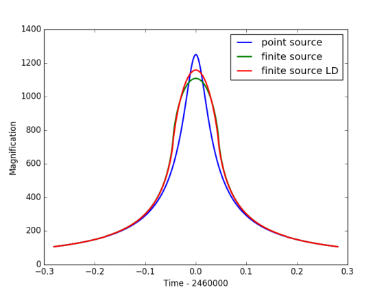
Figure 1: Example point-lens magnification curves. Blue line shows the point-source approximation (Paczyński curve) with high peak magnification. Green curve represents the finite source magnification curve ($\rho=0.0017$ and $u_{0}=0.0008$), while the red curve additionally includes the limb-darkening effect ($\Gamma=0.4$). The source codes used to produce this figure and Figures 2 and 4 are provided in the A. The values of all the parameters are given in the first few lines of each source code.

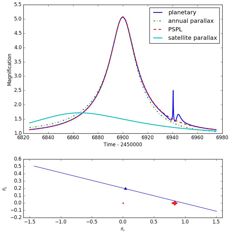
Figure 2: Example magnification curves (top panel): dashed red – point-source point-lens, solid blue – binary lens with planetary mass ratio ($q=0.001$, $s=1.5$), dot-dashed green – point-source point-lens curve affected by the annual parallax effect (relatively large value of $\pi_{\rm E}=0.61$), and solid cyan – point-source point-lens curve as seen by the Spitzer satellite (for the same parallax value). Note that the planetary model seen in the blue curve is significantly more complicated than a simple sum of two point-source point-lens models. The lower panel shows the source trajectory (blue) relative to caustics (red) for the planetary model from the top panel.

4.2 Finite source

We see from Equation 3, which is derived in the point-source point-lens limit, that the magnification would be infinite for $u=0$. In reality, the assumption of a point source is not valid, as every source has some finite, even if very small, angular size. For a typical bulge source, the angular source radius ($\theta_{\star}$) is a few ${\rm\mu arcsec}$, or about $0.001$ of $\theta_{\rm E}$ (e.g., Gaudi, 2012). Hence, if $u$ is smaller than a few times $\rho\equiv\theta_{\star}/\theta_{\rm E}$, then different parts of the source disk are magnified by significantly different amounts and the magnification differs from the point-source approximation (Witt and Mao, 1994). MulensModel  implements the finite source formalism by Gould (1994b), which was further extended to limb-darkened sources by Yoo et al. (2004). These methods are accurate as long as $\rho\lesssim 0.1$. The functions needed for finite source calculations were precomputed and cubic spline interpolation is used to find requested value. We have checked that relative interpolation errors are below $10^{-4}$. Alternatively, the user may request direct integration of underlying functions. See Figure 1 for example magnification curves with a finite source. The finite-source magnification curve is flattened at the peak compared to the Paczyński curve.

MulensModel  allows the user to make a few choices with regards to the finite source calculations. The limb-darkening coefficient can be provided following the $u$ convention (normalized by the central intensity) or the $\Gamma$ convention (normalized by the total flux; An et al., 2002). When fitting the model, the parameter $t_{\star}\equiv\rho t_{\rm E}$ may be a better choice than $\rho$, as $t_{\star}$ shows less correlation with other light-curve parameters (e.g. Yee et al., 2012). The value of $t_{\star}$ can be estimated as the half-width of the rounded part of the light curve, e.g., $2t_{\star}\sim 0.1~{}{\rm d}$ for the example in Figure 1.

4.3 Microlensing parallax

The parallax effect manifests in microlensing as a deflection of the trajectory of the lens relative to the source. The microlensing parallax $\boldsymbol{\pi_{\rm E}}$ is a 2D vector with magnitude equal to the relative lens-source parallax divided by $\theta_{\rm E}$. The direction of $\boldsymbol{\pi_{\rm E}}$ is the same as the relative lens-source proper motion.

If $\theta_{\rm E}$ is measured (e.g., by measuring finite source effects, see Yoo et al., 2004), the measurement of the microlensing parallax $\boldsymbol{\pi_{\rm E}}$ allows a direct measurement of the lens mass (Gould, 2000):

$$M=\frac{\theta_{\rm E}}{\kappa\pi_{\rm E}},$$

where $\kappa=4G/(c^{2}{\rm AU})=8.14~{}{\rm mas~{}M_{\odot}^{-1}}$ (${\rm mas}$ is short for milliarcsecond). Microlensing parallax also allows constraining the lens distance (Gould, 2000):

$$\frac{1}{D_{l}}=\pi_{\rm E}\theta_{\rm E}+\frac{1}{D_{s}}.$$

The two above equations allow translating parameters from the microlensing model (like mass ratio or projected separation of lens components) to physical properties of the lens system (masses of individual objects in ${\rm M_{\odot}}$ and projected separation in ${\rm AU}$). Hence, measuring, or at least constraining, the microlensing parallax plays an important role in characterizing the lens system.

Below we briefly discuss the microlensing parallax when it manifests as annual and satellite effects. In Figure 2 we show examples of magnification curves affected by both types of the microlensing parallax. Note that parallax affects the lens-source relative trajectory and hence can be included in both single-lens and double-lens models. Some of the model fitting algorithms require $\chi^{2}$ gradient calculation. MulensModel  allows calculation of $\chi^{2}$ gradient for point-source point-lens models including parallax models.

4.3.1 Annual parallax

The Paczyński curve assumes that the relative lens-source proper motion, as seen by the observer, is rectilinear as defined by Equations 4 and 5. For many microlensing events observed towards the Galactic bulge, the timescale $t_{\rm E}$ is shorter than $30~{}{\rm days}$ (Wyrzykowski et al., 2015). During this time, Earth’s orbital motion can be well-enough approximated as rectilinear. For longer events or events with particularly good photometric coverage, we may see the effect of Earth’s acceleration on the source-lens relative trajectory and, hence, in the light curve (An et al., 2002; Gould, 2004). The calculation of the impact of the annual microlensing parallax on the source trajectory requires calculating the projection of the Earth’s velocity onto the plane of the sky for a specified reference time for parameters $t_{0,{\rm par}}$ (Skowron et al., 2011). For point lenses the best choice is $t_{0,{\rm par}}\approx t_{0}$. For calculation of relative Earth-Sun positions we use high-accuracy ephemerides included in Astropy package (Astropy Collaboration et al., 2013, 2018).

4.3.2 Satellite parallax

Another method to measure the microlensing parallax is to observe the same event from at least two well-separated locations (Refsdal, 1966; Gould, 1994a). Typical scales of the bulge microlensing translate to the optimal separation of the satellite projected towards the bulge of about $1~{}{\rm AU}$. Both the Spitzer (Zhu et al., 2017b) and K2 (Henderson et al., 2016) satellite missions meet this criterion and have observed many microlensing events in recent years. Calculating the satellite parallax effect requires calculating the projection of the Earth-satellite separation on the plane of the sky. For extracting accurate satellite positions we use JPL Horizons e-mail system (Giorgini et al., 1996) and give detailed instructions how this system should be accessed (file documents/Horizons_manual.md).

5 Binary lenses

A binary lens consists of two components that are often parameterized by their mass ratio $q\equiv m_{2}/m_{1}$ and their projected separation $s$ (defined as a fraction of the Einstein ring radius of the combined mass). The magnification calculations for a binary lens are implemented in the BinaryLens class.

5.1 Lens equation

The addition of a second mass to the lensing system significantly changes the microlensing calculations. For point lenses discussed in Section 4, we treated source and image positions as one-dimensional thanks to the symmetry of the problem. The symmetry is broken by the second lens and we have to use two-dimensional coordinates. It is most convenient to use complex numbers to represent the coordinates (Witt, 1990). Let $\zeta$, $z$, $z_{1}$, and $z_{2}$ be the source position, image position, and positions of the two lenses, respectively. The lens equation is then:

$$\zeta=z+\frac{m_{1}}{\bar{z_{1}}-\bar{z}}+\frac{m_{2}}{\bar{z_{2}}-\bar{z}}.$$

The above equation can be converted into a fifth-order complex polynomial and then solved numerically, though one has to check if all five solutions of the polynomial are also solutions of the lens equation, of which there are either three or five. MulensModel  uses polynomial coefficients given by Witt and Mao (1995) and the polynomial is solved using the Bozza et al. (2018) implementation of the Skowron and Gould (2012) root solver. The magnification $A$ is

$$A=\sum\frac{1}{\left|\det J\right|},$$ (6)

where summation is done over all images, and $J$ is the Jacobian of the lens equation. The example magnification curve for a binary-lens event with planetary mass ratio is shown in Figure 2 by the blue solid curve.

The source positions corresponding to $\det J=0$ define a caustic curve, on which the point source magnification would be infinite. Because the magnification diverges near a caustic, the physical size of the source and its limb-darkening significantly affect the total observed magnification within a few source radii of a caustic. As noted in Section 4.2, for a point lens the magnification $\rightarrow\infty$ at a single point $u=0$. Thus, for a point lens the caustic is just a point (same as the lens position), but for binary lenses the caustic curve expands to a series of edges that describe one, two, or three enclosed regions (Erdl and Schneider, 1993). Hence, the chances of detecting the finite source effect are much higher for binary lenses.

5.2 Finite Source

The simplest approach to the finite-source binary-lens magnification calculations is a direct two-dimensional integration but this approach is computationally very inefficient. Far from the caustic, it is sufficient to approximate the source as a single point, and this is the fastest method for calculating the magnification. Below we discuss various approaches to calculating the finite-source binary-lens magnification in order of increasing accuracy (near a caustic) and correspondingly, increasing computation time.

5.2.1 Taylor expansion

After the point source approximation, the next fastest approach is to calculate the magnification using the quadrupole or hexadecapole approximation of the Taylor expansion of the lensing potential (Gould, 2008; Pejcha and Heyrovský, 2009). Only nine and thirteen point-source lens equation computations are required in the quadrupole and hexadecapole approximation, respectively. The approximation is generally valid and useful for source positions that are between a few and tens of source radii from the caustic. As described in Gould (2008), the exact region of validity must be determined individually for each light curve.

5.2.2 Contour integration

The 2D area of an image of constant surface-brightness source can be calculated by integrating over the 1D image contour thanks to Green’s theorem (Gould and Gaucherel, 1997). It is faster to integrate over one dimension compared to two dimensions. Hence, the contour integration is an important approach to finite-source binary-lens calculations.

There are several implementation problems of contour integration that have been solved over the years. MulensModel implements two of the available contour integration methods. The first method is Adaptive Contouring by Dominik (2007) that uses adaptive grid size to find contours of all images. The second method is VBBL by Bozza (2010) and Bozza et al. (2018) that improves the accuracy of integration and controls the residuals, which allows optimal sampling of the source. In the example cases tested by (Bozza, 2010), the number of lens equation solutions was typically a few times larger than the resulting magnification for uniform source. The limb darkening effect required a few times more lens equation solutions. Bozza et al. (2018) presented a method to decide when to use faster point source calculations instead of finite source calculations. MulensModel  does not use this method at this time, but may add it as an option during future development. Both Adaptive Contouring and VBBL were implemented by their authors in C or C++ and MulensModel  calls these codes.

6 Performance

To test the code performance, we benchmark the $\chi^{2}$ calculation function for point-source point-lens event with a single dataset at a time. The datasets had $10^{2}$, $10^{3}$, and $10^{4}$ datapoints. The largest dataset is on the order of largest datasets that will be analyzed in foreseeable future. We tested both rectilinear motion and annual parallax events. To make the benchmark meaningful, we wrote short $\chi^{2}$ function for event without annual parallax using numpy package. The numpy-based function implements Paczyński curve, performs linear regression to derive source and blending flux, calculates predicted flux values, and evaluates $\chi^{2}$. The goal should be that additional calculations that are performed in the high-level package MulensModel  add as small overhead as possible.

We run the benchmark on a desktop computer with a single socket, 10 core modern processor (Intel Xeon E5-2630 v4 2.20GHz). The testing environment was Linux Centos distribution with python 3.6.5 (GCC 7.2.0), numpy 1.14.3, scipy 1.1.0, and astropy 3.0.2. The testing was performed using perf benchmarking package version 1.5.1. We run MulensModel  twice. First, the $\chi^{2}$ contributions of all the points are added using accurate floating point sum of values (i.e., math.fsum), which is the default setting. Second, the $\chi^{2}$ contributions are added using numpy.sum function which can be less accurate. For comparison with MulensModel  version 1.4.0 presented here, we also tested pyLIMA version 1.0.0. We note that pyLIMA does not specify conventions for model parameters directly, and we had to change signs of $\boldsymbol{\pi_{\rm E}}$ components to obtain results consistent with the Skowron et al. (2011) convention, i.e., as if the components are in S and W directions, not N and E. The codes used to run the benchmark and raw test results are included in MulensModel  distribution (see examples/run_time_tests/).

Figure 3 shows ratio of the run time relative to the run time of rectilinear model $\chi^{2}$ calculation with numpy and ideally should be close to 1. The run times with numpy are $0.13~{}{\rm ms}$, $0.18~{}{\rm ms}$, and $0.71~{}{\rm ms}$ for $10^{2}$, $10^{3}$, and $10^{4}$ datapoints, respectively. In all cases, the ratios are below 3.5. For $10^{2}$ and $10^{3}$ points, the differences between MulensModel  and pyLIMA are comparable to standard deviations. For $10^{4}$ MulensModel  calculation with numpy.sum is clearly the fastest.

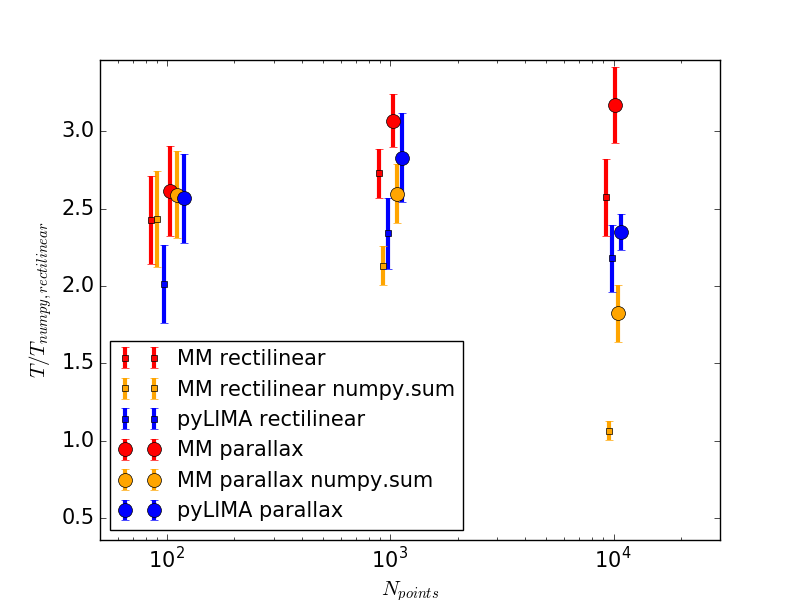
Figure 3: Benchmark comparing execution times for MulensModel  (red and orange points) and pyLIMA (blue points). The run time is given relative to run time of the simple $\chi^{2}$ calculation performed in numpy. Small squares present models with rectilinear motion, while large circles indicate annual parallax models. For MulensModel  we show both default calculation (red points) as well as faster calculation that uses numpy.sum instead of math.fsum (orange points). X axis coordinates are slightly shifted for better visibility.

7 Additional features

The main goal of MulensModel  is to calculate magnification curves that are used for model fitting. The code also provides a number of additional convenience functions. These functions fall outside the main scope of the code, but the user may find them useful. Thus, we describe them here.

7.1 Plotting

MulensModel  offers several built-in plotting functions to facilitate the visualization of models, data, and the model residuals. In addition to the magnification curves shown in Figures 1 and 2, MulensModel  makes it easy for the user to plot data with a given model. For each dataset the optimum values of $F_{S}$ and $F_{B}$ are found and the brightness measurements are scaled to the same magnitude system (Equation 1). Figure 4 shows the OGLE and MOA data for OGLE-2003-BLG-235/MOA-2003-BLG-53 (Bond et al., 2004) and the model light curve. There are also built-in functions for plotting the caustics and the trajectory of the source relative to the lens.

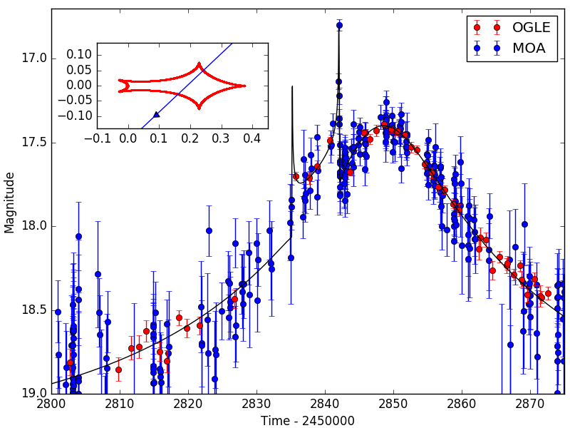
Figure 4: Data for OGLE-2003-BLG-235/MOA-2003-BLG-53 shown with a model generated with MulensModel. The model is based on Bond et al. (2004), but the exact parameters were adjusted to better approximate the data. Only the flux parameters were fit by MulensModel. Photometry was acquired from NASA Exoplanet Archive. The inset shows the source trajectory (blue) relative to caustic (red).

7.2 Reparameterization

There are multiple sets of parameters that can be used for model fitting and the optimal choice depends on the specific event being considered. In addition to $\rho\leftrightarrow t_{\star}$ reparameterization described in Section 4.2, MulensModel  allows use of the effective timescale ($t_{\rm eff}\equiv u_{0}t_{\rm E}$) instead of either $u_{0}$ or $t_{\rm E}$.

7.3 Hypothetical Systems

The mulensobjects submodule allows the user to easily calculate microlensing quantities by defining a physical lens-source system. For example, the user may specify a lens mass, distances to the source and lens, and the relative lens-source proper motion and then retrieve $t_{\rm E}$ or various projections of the Einstein radius.

8 Future development

While version 1.4.0 of MulensModel  allows a wide variety of events to be analyzed, we can envision many avenues for updates and expansions to the code, some of which we briefly outlined below.

8.1 Additional magnification calculation methods

There are several other methods for calculating the source magnification when finite source effects are significant. These may be more accurate or more efficient than those currently implemented, depending on the exact case. For example, for point lenses in which $\rho\gtrsim 0.1$, the Lee et al. (2009) method should be used. In the case of binary lenses, there are other contour integration algorithms (e.g. Dong et al., 2009). In addition to contour integration, the finite-source binary-lens magnification can be calculated using the inverse-ray shooting method (Kayser et al., 1986). The details of the inverse-ray shooting method have been improved over the years (e.g. Vermaak, 2000; Dong et al., 2006; Bennett, 2010). Recently, Cassan (2017) proposed a method to increase efficiency of Taylor expansion calculations. Implementing some or all of these methods could be a direction for future development.

8.2 Additional parameterizations

MulensModel  is built using the center-of-mass coordinate system. However, there are a number of other possible parameterizations of the event that can make fitting easier and more efficient. For example, Cassan (2008) proposed a binary lens parameterization that uses the epochs of the caustic crossings, which are well measured, and two coordinates along the caustic as fitting parameters in place of, e.g., $t_{0}$, $u_{0}$, $t_{\rm E}$, and $\alpha$. Penny (2014) presented a way to optimize planetary events simulations. The properties of caustics in planetary mass ratio regime were studied by Chung et al. (2005) and Han (2006). The parameters derived by them can be useful in fitting particular events and in some cases one can estimate event properties based on a simple light curve inspection (Gould and Loeb, 1992; Poleski et al., 2014b). Even for point-lens events one may want to use different sets of microlensing parameters to speed-up the calculations (Yee et al., 2012). Re-parameterization not only makes exploration of the parameter space easier, but in doing so improves the probability that all alternative, degenerate models have been found and considered. Since the user defines the minimization algorithm, the user can define a likelihood function that converts an arbitrary parameter set into the center-of-mass coordinate system used by MulensModel  and then calculate and return the $\chi^{2}$. However, a path for future development would be to create built-in functions to convert between various parameterizations.

8.3 Higher-order Effects and Triple Lenses

There are additional, higher-order effects that we plan to implement in the near future: binary sources (two luminous sources), the xallarap effect (Griest and Hu, 1992; Dominik, 1998), and two-parameter limb-darkening. We note that currently there is no capability in MulensModel  for astrometric microlensing calculations (Belokurov and Evans, 2002; Sahu et al., 2017) but it can be added in future.

Another obvious path for future development is adding triple-lens models. The serious limitation in implementing the finite-source triple-lens models is the lack of deep understanding of triple-lens caustic structures (see, e.g., Daněk and Heyrovský, 2015; Luhn et al., 2016). For numerical contour integration methods, this leads to problems with correctly matching up the points along the contours. The problem is particularly severe near swallowtail and butterfly morphologies. Also the model degeneracies are more severe (Song et al., 2014). Additionally, in some cases, the solutions of 10-th order polynomial can be numerically unstable (Han and Han, 2002; Bennett, 2010).

8.4 WFIRST Data Analysis Challenges

A series of Data Analysis Challenges in advance of WFIRST are currently underway, and we hope that MulensModel will serve as a useful tool for those challenges and for development of the WFIRST analysis pipeline. The immediate, future development of MulensModel  will likely be driven by ensuring that MulensModel  can be used to address the problems posed by the Data Analysis Challenges. Thus, most likely, the next round of development will focus on implementing orbital motion, additional model parameterizations, and triple lenses. We also anticipate that the Data Analysis Challenges will reveal new pathways for future development on MulensModel.

We welcome community feedback on the current status of the code, requests of features to be added, and help in developing the code.

Appendix A Source codes

Below we present the source codes used to prepare the Figures 1, 2, and 4. The figures include a few higher order effects and subpanels presenting caustics, yet the codes are succinct.

Listing 1: Code used to prepare Figure 1

⬇

"""

Create Figure 1.

Example point-source magnification curves.

"""

from matplotlib import pyplot

from MulensModel import Model

# Define model parameters.

t_0 = 2460000

params_ps = {’t_0’: t_0, ’u_0’: 0.0008, ’t_E’: 30.}

t_star = 0.051 # Day is default unit for t_E and t_star.

gamma = 0.4 # This is limb darkening coefficient.

params_fs = {**params_ps, ’t_star’: t_star}

# Set models settings for:

model_ps = Model(params_ps) # point source,

model_fs = Model(params_fs) # finite source,

model_fs_ld = Model(params_fs) # and finite source with limb darkening.

# Specify which finite source methods are used and when:

t_1 = t_0 - 3.5 * t_star

t_2 = t_0 + 3.5 * t_star

model_fs.set_magnification_methods([t_1, ’finite_source_uniform_Gould94’, t_2])

model_fs_ld.set_magnification_methods([t_1, ’finite_source_LD_Yoo04’, t_2])

# Plot the magnification curves.

plot_kwargs = {’t_start’: t_0-5.5*t_star, ’t_stop’: t_0+5.5*t_star,

’subtract_2460000’: True, ’lw’: 2.}

model_ps.plot_magnification(label=’point source’, **plot_kwargs)

model_fs.plot_magnification(label=’finite source’, **plot_kwargs)

model_fs_ld.plot_magnification(

gamma=gamma, label=’finite source LD’, **plot_kwargs)

pyplot.legend(loc=’best’)

pyplot.savefig(’figure_1.png’)

Listing 2: Code used to prepare Figure 2

⬇

"""

Create Figure 2.

Example magnification curves.

"""

from matplotlib import pyplot

import os

from MulensModel import Model, SatelliteSkyCoord, MODULE_PATH

# Define model parameters.

params = {’t_0’: 2456900, ’u_0’: 0.2, ’t_E’: 50.}

params_pi_E = {’pi_E_N’: 0.35, ’pi_E_E’: 0.5}

params_planet = {’rho’: 0.002, ’s’: 1.5, ’q’: 0.001, ’alpha’: 348.1}

ra_dec = ’18:00:00.00 -28:30:00.0’

# Set models and satellite settings.

model_pspl = Model(params)

model_planet = Model({**params, **params_planet})

# Calculate finite source magnification using VBBL method for this

# range of dates:

model_planet.set_magnification_methods([2456937, ’VBBL’, 2456945])

# Parallax settings:

model_parallax = Model({**params, **params_pi_E}, coords=ra_dec)

model_parallax.parallax(earth_orbital=True, satellite=True)

satellite = SatelliteSkyCoord(

os.path.join(

MODULE_PATH, ’data/ephemeris_files’, ’Spitzer_ephemeris_01.dat’))

# This file gives the Spitzer ephemeris and is part of MulensModel package.

# Plot the magnification curves.

plot_kwargs = {’subtract_2450000’: True, ’lw’: 2.}

pyplot.figure(figsize=(8,8))

pyplot.axes([0.1, 0.43, 0.85, 0.55])

model_planet.plot_magnification(label=’planetary’, **plot_kwargs)

model_parallax.plot_magnification(

label=’annual parallax’, linestyle=’-.’, **plot_kwargs)

model_pspl.plot_magnification(label=’PSPL’, linestyle=’--’, **plot_kwargs)

model_parallax.plot_magnification(

label=’satellite parallax’, satellite_skycoord=satellite, **plot_kwargs)

pyplot.legend(loc=’best’)

pyplot.axes([0.1, 0.07, 0.85, 0.25]) # Lower panel starts here.

model_planet.plot_trajectory(caustics=True)

pyplot.xlim(-1.52, 1.61)

pyplot.xlabel(r"$\theta_x$")

pyplot.ylabel(r"$\theta_y$")

pyplot.savefig(’figure_2.png’)

Listing 3: Code used to prepare Figure 4

⬇

"""

Creates Figure 4.

This example shows OGLE-2003-BLG-235/MOA-2003-BLG-53,

the first microlensing planet.

"""

from matplotlib import pyplot

import os

from MulensModel import MulensData, Model, Event, MODULE_PATH

# Import data

data_dir = os.path.join(MODULE_PATH, ’data’, ’photometry_files’, ’OB03235’)

OGLE_data = MulensData(

file_name=os.path.join(data_dir, ’OB03235_OGLE.tbl.txt’),

comments=[’\\’, ’|’])

MOA_data = MulensData(

file_name=os.path.join(data_dir, ’OB03235_MOA.tbl.txt’),

comments=[’\\’, ’|’], phot_fmt=’flux’)

# Define a model with a 2-body lens (these parameters slightly differ

# from Bond et al. 2004):

model_1S2L = Model({’t_0’: 2452848.06, ’u_0’: 0.1317, ’t_E’: 61.5,

’rho’: 0.00096, ’q’: 0.0039, ’s’: 1.120, ’alpha’: 223.72})

# Since rho is set, define a time range and method to apply finite

# source effects:

model_1S2L.set_magnification_methods([2452833., ’VBBL’, 2452845.])

# Combine the data and model into an Event:

my_event = Event(datasets=[OGLE_data, MOA_data], model=model_1S2L)

# Make the plot:

t_range = [2452800., 2452875.]

pyplot.axes([0.09, 0.08, 0.9, 0.9])

my_event.plot_data(

subtract_2450000=True, label_list=[’OGLE’, ’MOA’],

color_list=[’red’, ’blue’], zorder_list=[2, 1], s=6)

my_event.plot_model(

subtract_2450000=True, t_range=t_range, n_epochs=4000, color=’black’)

pyplot.legend(loc=’best’)

pyplot.xlim(t_range[0]-2450000., t_range[1]-2450000.)

pyplot.ylim(19.0, 16.7)

pyplot.axes([0.17, 0.7, 0.3, 0.2]) # Figure inset stars here.

model_1S2L.plot_trajectory(caustics=True)

pyplot.xlim(-0.1, 0.45)

pyplot.ylim(-0.14, 0.14)

pyplot.savefig(’figure_4.png’)

Appendix B Public microlensing datasets

MulensModel  is meant to be used for analysis of real microlensing events but also exploring novel solutions to the computational challenges faced by microlensing. Conducting such an exploration requires access to photometric data of real microlensing events. There now exist several public data sets, which might be analyzed or used to study these problems. Because a list of these data sets has not been previously compiled, we review here the public time-series photometry of microlensing events starting from newest datasets.

The KMTNet survey has operated telescopes on three continents since 2015 (Kim et al., 2016). The photometry of events from 2015 commissioning season and 2016 data for K2 Campaign 9 footprint are public (Kim et al., 2018a, b) (altogether 841 clear events and 266 classified as possible) and future datasets will also be publicly released. In 2015 and 2016 the microlensing survey was conducted using UKIRT telescope (Shvartzvald et al., 2017a) and all $18\times 10^{6}$ aperture photometry light curves were released. Similarly, aperture photometry for all sources observed between 2010 and 2015 by the VVV survey (Minniti et al., 2010) is also public.

The public time-series images are available for events observed by Spitzer and K2 satellite missions. Spitzer has conducted microlensing campaigns since 2014, while K2 conducted the first space-based microlensing survey in its Campaign 9 (Henderson et al., 2016) with additional targets observed in Campaign 11. Extracting photometry from both Spitzer and K2 images of Galactic bulge requires specialized techniques (Calchi Novati et al., 2015b; Zhu et al., 2017a).

The sample of 3718 OGLE-III survey (Udalski et al., 2008) events used for Galactic bulge structure study was presented by Wyrzykowski et al. (2015). These events are primarily point-source point-lens events, but parallax events and some binary events are present in this sample. The MOA-II survey (Sako et al., 2008) sample consists of 474 events (Sumi et al., 2013) and some of these are common with Wyrzykowski et al. (2015) sample. Similarly, Sumi et al. (2006) released 122 light-curves from the OGLE-II survey. A sample of 214 OGLE-II light-curves was published by Udalski et al. (2000). Additional OGLE-II microlensing events are present in the Wozniak et al. (2002) catalog of $2\times 10^{5}$ variable sources. Also Thomas et al. (2005) released 564 light-curves from the MACHO project bulge study.

The photometry of events that were published as planetary microlensing can be accessed via the NASA Exoplanet Archive.

References

- An et al. (2002) An, J.H., Albrow, M.D., Beaulieu, J.P., Caldwell, J.A.R., DePoy, D.L., Dominik, M., Gaudi, B.S., Gould, A., Greenhill, J., Hill, K., Kane, S., Martin, R., Menzies, J., Pogge, R.W., Pollard, K.R., Sackett, P.D., Sahu, K.C., Vermaak, P., Watson, R., Williams, A., 2002. First Microlens Mass Measurement: PLANET Photometry of EROS BLG-2000-5. ApJ 572, 521–539. astro-ph/0110095.
- Astropy Collaboration et al. (2018) Astropy Collaboration, Price-Whelan, A.M., Sipőcz, B.M., Günther, H.M., Lim, P.L., Crawford, S.M., Conseil, S., Shupe, D.L., Craig, M.W., Dencheva, N., Ginsburg, A., VanderPlas, J.T., Bradley, L.D., Pérez-Suárez, D., de Val-Borro, M., Aldcroft, T.L., Cruz, K.L., Robitaille, T.P., Tollerud, E.J., Ardelean, C., Babej, T., Bach, Y.P., Bachetti, M., Bakanov, A.V., Bamford, S.P., Barentsen, G., Barmby, P., Baumbach, A., Berry, K.L., Biscani, F., Boquien, M., Bostroem, K.A., Bouma, L.G., Brammer, G.B., Bray, E.M., Breytenbach, H., Buddelmeijer, H., Burke, D.J., Calderone, G., Cano Rodríguez, J.L., Cara, M., Cardoso, J.V.M., Cheedella, S., Copin, Y., Corrales, L., Crichton, D., D’Avella, D., Deil, C., Depagne, É., Dietrich, J.P., Donath, A., Droettboom, M., Earl, N., Erben, T., Fabbro, S., Ferreira, L.A., Finethy, T., Fox, R.T., Garrison, L.H., Gibbons, S.L.J., Goldstein, D.A., Gommers, R., Greco, J.P., Greenfield, P., Groener, A.M., Grollier, F., Hagen, A., Hirst, P., Homeier, D., Horton, A.J., Hosseinzadeh, G., Hu, L., Hunkeler, J.S., Ivezić, Ž., Jain, A., Jenness, T., Kanarek, G., Kendrew, S., Kern, N.S., Kerzendorf, W.E., Khvalko, A., King, J., Kirkby, D., Kulkarni, A.M., Kumar, A., Lee, A., Lenz, D., Littlefair, S.P., Ma, Z., Macleod, D.M., Mastropietro, M., McCully, C., Montagnac, S., Morris, B.M., Mueller, M., Mumford, S.J., Muna, D., Murphy, N.A., Nelson, S., Nguyen, G.H., Ninan, J.P., Nöthe, M., Ogaz, S., Oh, S., Parejko, J.K., Parley, N., Pascual, S., Patil, R., Patil, A.A., Plunkett, A.L., Prochaska, J.X., Rastogi, T., Reddy Janga, V., Sabater, J., Sakurikar, P., Seifert, M., Sherbert, L.E., Sherwood-Taylor, H., Shih, A.Y., Sick, J., Silbiger, M.T., Singanamalla, S., Singer, L.P., Sladen, P.H., Sooley, K.A., Sornarajah, S., Streicher, O., Teuben, P., Thomas, S.W., Tremblay, G.R., Turner, J.E.H., Terrón, V., van Kerkwijk, M.H., de la Vega, A., Watkins, L.L., Weaver, B.A., Whitmore, J.B., Woillez, J., Zabalza, V., Astropy Contributors, 2018. The Astropy Project: Building an Open-science Project and Status of the v2.0 Core Package. AJ 156, 123. 1801.02634.
- Astropy Collaboration et al. (2013) Astropy Collaboration, Robitaille, T.P., Tollerud, E.J., Greenfield, P., Droettboom, M., Bray, E., Aldcroft, T., Davis, M., Ginsburg, A., Price-Whelan, A.M., Kerzendorf, W.E., Conley, A., Crighton, N., Barbary, K., Muna, D., Ferguson, H., Grollier, F., Parikh, M.M., Nair, P.H., Unther, H.M., Deil, C., Woillez, J., Conseil, S., Kramer, R., Turner, J.E.H., Singer, L., Fox, R., Weaver, B.A., Zabalza, V., Edwards, Z.I., Azalee Bostroem, K., Burke, D.J., Casey, A.R., Crawford, S.M., Dencheva, N., Ely, J., Jenness, T., Labrie, K., Lim, P.L., Pierfederici, F., Pontzen, A., Ptak, A., Refsdal, B., Servillat, M., Streicher, O., 2013. Astropy: A community Python package for astronomy. A&A 558, A33. 1307.6212.
- Bachelet et al. (2017) Bachelet, E., Norbury, M., Bozza, V., Street, R., 2017. pyLIMA: An Open-source Package for Microlensing Modeling. I. Presentation of the Software and Analysis of Single-lens Models. AJ 154, 203.
- Beaulieu et al. (2006) Beaulieu, J.P., Bennett, D.P., Fouqué, P., Williams, A., Dominik, M., Jørgensen, U.G., Kubas, D., Cassan, A., Coutures, C., Greenhill, J., Hill, K., Menzies, J., Sackett, P.D., Albrow, M., Brillant, S., Caldwell, J.A.R., Calitz, J.J., Cook, K.H., Corrales, E., Desort, M., Dieters, S., Dominis, D., Donatowicz, J., Hoffman, M., Kane, S., Marquette, J.B., Martin, R., Meintjes, P., Pollard, K., Sahu, K., Vinter, C., Wambsganss, J., Woller, K., Horne, K., Steele, I., Bramich, D.M., Burgdorf, M., Snodgrass, C., Bode, M., Udalski, A., Szymański, M.K., Kubiak, M., Wiȩckowski, T., Pietrzyński, G., Soszyński, I., Szewczyk, O., Wyrzykowski, Ł., Paczyński, B., Abe, F., Bond, I.A., Britton, T.R., Gilmore, A.C., Hearnshaw, J.B., Itow, Y., Kamiya, K., Kilmartin, P.M., Korpela, A.V., Masuda, K., Matsubara, Y., Motomura, M., Muraki, Y., Nakamura, S., Okada, C., Ohnishi, K., Rattenbury, N.J., Sako, T., Sato, S., Sasaki, M., Sekiguchi, T., Sullivan, D.J., Tristram, P.J., Yock, P.C.M., Yoshioka, T., 2006. Discovery of a cool planet of 5.5 Earth masses through gravitational microlensing. Nature 439, 437–440. arXiv:astro-ph/0601563.
- Belokurov and Evans (2002) Belokurov, V.A., Evans, N.W., 2002. Astrometric microlensing with the GAIA satellite. MNRAS 331, 649–665. astro-ph/0112243.
- Bennett (2010) Bennett, D.P., 2010. An Efficient Method for Modeling High-magnification Planetary Microlensing Events. ApJ 716, 1408–1422. 0911.2703.
- Bensby et al. (2017) Bensby, T., Feltzing, S., Gould, A., Yee, J.C., Johnson, J.A., Asplund, M., Meléndez, J., Lucatello, S., Howes, L.M., McWilliam, A., Udalski, A., Szymański, M.K., Soszyński, I., Poleski, R., Wyrzykowski, Ł., Ulaczyk, K., Kozłowski, S., Pietrukowicz, P., Skowron, J., Mróz, P., Pawlak, M., Abe, F., Asakura, Y., Bhattacharya, A., Bond, I.A., Bennett, D.P., Hirao, Y., Nagakane, M., Koshimoto, N., Sumi, T., Suzuki, D., Tristram, P.J., 2017. Chemical evolution of the Galactic bulge as traced by microlensed dwarf and subgiant stars. VI. Age and abundance structure of the stellar populations in the central sub-kpc of the Milky Way. A&A 605, A89. 1702.02971.
- Bond et al. (2017) Bond, I.A., Bennett, D.P., Sumi, T., Udalski, A., Suzuki, D., Rattenbury, N.J., Bozza, V., Koshimoto, N., Abe, F., Asakura, Y., Barry, R.K., Bhattacharya, A., Donachie, M., Evans, P., Fukui, A., Hirao, Y., Itow, Y., Li, M.C.A., Ling, C.H., Masuda, K., Matsubara, Y., Muraki, Y., Nagakane, M., Ohnishi, K., Ranc, C., Saito, T., Sharan, A., Sullivan, D.J., Tristram, P.J., Yamada, T., Yamada, T., Yonehara, A., Skowron, J., Szymański, M.K., Poleski, R., Mróz, P., Soszyński, I., Pietrukowicz, P., Kozłowski, S., Ulaczyk, K., Pawlak, M., 2017. The lowest mass ratio planetary microlens: OGLE 2016-BLG-1195Lb. MNRAS 469, 2434–2440. 1703.08639.
- Bond et al. (2004) Bond, I.A., Udalski, A., Jaroszyński, M., Rattenbury, N.J., Paczyński, B., Soszyński, I., Wyrzykowski, L., Szymański, M.K., Kubiak, M., Szewczyk, O., Żebruń, K., Pietrzyński, G., Abe, F., Bennett, D.P., Eguchi, S., Furuta, Y., Hearnshaw, J.B., Kamiya, K., Kilmartin, P.M., Kurata, Y., Masuda, K., Matsubara, Y., Muraki, Y., Noda, S., Okajima, K., Sako, T., Sekiguchi, T., Sullivan, D.J., Sumi, T., Tristram, P.J., Yanagisawa, T., Yock, P.C.M., OGLE Collaboration, 2004. OGLE 2003-BLG-235/MOA 2003-BLG-53: A Planetary Microlensing Event. ApJL 606, L155–L158. arXiv:astro-ph/0404309.
- Bozza (2010) Bozza, V., 2010. Microlensing with an advanced contour integration algorithm: Green’s theorem to third order, error control, optimal sampling and limb darkening. MNRAS 408, 2188–2200. 1004.2796.
- Bozza et al. (2018) Bozza, V., Bachelet, E., Bartolić, F., Heintz, T.M., Hoag, A.R., Hundertmark, M., 2018. VBBINARYLENSING: a public package for microlensing light-curve computation. MNRAS 479, 5157–5167. 1805.05653.
- Calchi Novati et al. (2015a) Calchi Novati, S., Gould, A., Udalski, A., Menzies, J.W., Bond, I.A., Shvartzvald, Y., Street, R.A., Hundertmark, M., Beichman, C.A., Yee, J.C., Carey, S., Poleski, R., Skowron, J., Kozłowski, S., Mróz, P., Pietrukowicz, P., Pietrzyński, G., Szymański, M.K., Soszyński, I., Ulaczyk, K., Wyrzykowski, Ł., OGLE Collaboration, Albrow, M., Beaulieu, J.P., Caldwell, J.A.R., Cassan, A., Coutures, C., Danielski, C., Dominis Prester, D., Donatowicz, J., Lončarić, K., McDougall, A., Morales, J.C., Ranc, C., Zhu, W., PLANET Collaboration, Abe, F., Barry, R.K., Bennett, D.P., Bhattacharya, A., Fukunaga, D., Inayama, K., Koshimoto, N., Namba, S., Sumi, T., Suzuki, D., Tristram, P.J., Wakiyama, Y., Yonehara, A., The MOA Collaboration, Maoz, D., Kaspi, S., Friedmann, M., Wise Group, Bachelet, E., Figuera Jaimes, R., Bramich, D.M., Tsapras, Y., Horne, K., Snodgrass, C., Wambsganss, J., Steele, I.A., Kains, N., RoboNet Collaboration, Bozza, V., Dominik, M., Jørgensen, U.G., Alsubai, K.A., Ciceri, S., D’Ago, G., Haugbølle, T., Hessman, F.V., Hinse, T.C., Juncher, D., Korhonen, H., Mancini, L., Popovas, A., Rabus, M., Rahvar, S., Scarpetta, G., Schmidt, R.W., Skottfelt, J., Southworth, J., Starkey, D., Surdej, J., Wertz, O., Zarucki, M., MiNDSTEp Consortium, Gaudi, B.S., Pogge, R.W., DePoy, D.L., FUN Collaboration, 2015a. Pathway to the Galactic Distribution of Planets: Combined Spitzer and Ground-Based Microlens Parallax Measurements of 21 Single-Lens Events. ApJ 804, 20. 1411.7378.
- Calchi Novati et al. (2015b) Calchi Novati, S., Gould, A., Yee, J.C., Beichman, C., Bryden, G., Carey, S., Fausnaugh, M., Gaudi, B.S., Henderson, C.B., Pogge, R.W., Shvartzvald, Y., Wibking, B., Zhu, W., Spitzer Team, Udalski, A., Poleski, R., Pawlak, M., Szymański, M.K., Skowron, J., Mróz, P., Kozłowski, S., Wyrzykowski, Ł., Pietrukowicz, P., Pietrzyński, G., Soszyński, I., Ulaczyk, K., OGLE Group, 2015b. Spitzer IRAC Photometry for Time Series in Crowded Fields. ApJ 814, 92. 1509.00037.
- Cassan (2008) Cassan, A., 2008. An alternative parameterisation for binary-lens caustic-crossing events. A&A 491, 587–595. 0808.1527.
- Cassan (2017) Cassan, A., 2017. Fast computation of quadrupole and hexadecapole approximations in microlensing with a single point-source evaluation. MNRAS 468, 3993–3999. 1703.03600.
- Chung et al. (2005) Chung, S.J., Han, C., Park, B.G., Kim, D., Kang, S., Ryu, Y.H., Kim, K.M., Jeon, Y.B., Lee, D.W., Chang, K., Lee, W.B., Kang, Y.H., 2005. Properties of Central Caustics in Planetary Microlensing. ApJ 630, 535–542. arXiv:astro-ph/0505363.
- Coughlin et al. (2016) Coughlin, J.L., Mullally, F., Thompson, S.E., Rowe, J.F., Burke, C.J., Latham, D.W., Batalha, N.M., Ofir, A., Quarles, B.L., Henze, C.E., Wolfgang, A., Caldwell, D.A., Bryson, S.T., Shporer, A., Catanzarite, J., Akeson, R., Barclay, T., Borucki, W.J., Boyajian, T.S., Campbell, J.R., Christiansen, J.L., Girouard, F.R., Haas, M.R., Howell, S.B., Huber, D., Jenkins, J.M., Li, J., Patil-Sabale, A., Quintana, E.V., Ramirez, S., Seader, S., Smith, J.C., Tenenbaum, P., Twicken, J.D., Zamudio, K.A., 2016. Planetary Candidates Observed by Kepler. VII. The First Fully Uniform Catalog Based on the Entire 48-month Data Set (Q1-Q17 DR24). ApJS 224, 12. 1512.06149.
- Daněk and Heyrovský (2015) Daněk, K., Heyrovský, D., 2015. Critical Curves and Caustics of Triple-lens Models. ApJ 806, 99. 1501.06519.
- Dominik (1998) Dominik, M., 1998. Galactic microlensing with rotating binaries. A&A 329, 361–374. astro-ph/9702039.
- Dominik (1999) Dominik, M., 1999. The binary gravitational lens and its extreme cases. A&A 349, 108–125. astro-ph/9903014.
- Dominik (2007) Dominik, M., 2007. Adaptive contouring - an efficient way to calculate microlensing light curves of extended sources. MNRAS 377, 1679–1688. astro-ph/0703305.
- Dong et al. (2009) Dong, S., Bond, I.A., Gould, A., Kozłowski, S., Miyake, N., Gaudi, B.S., Bennett, D.P., Abe, F., Gilmore, A.C., Fukui, A., Furusawa, K., Hearnshaw, J.B., Itow, Y., Kamiya, K., Kilmartin, P.M., Korpela, A., Lin, W., Ling, C.H., Masuda, K., Matsubara, Y., Muraki, Y., Nagaya, M., Ohnishi, K., Okumura, T., Perrott, Y.C., Rattenbury, N., Saito, T., Sako, T., Sato, S., Skuljan, L., Sullivan, D.J., Sumi, T., Sweatman, W., Tristram, P.J., Yock, P.C.M., MOA Collaboration, Bolt, G., Christie, G.W., DePoy, D.L., Han, C., Janczak, J., Lee, C.U., Mallia, F., McCormick, J., Monard, B., Maury, A., Natusch, T., Park, B.G., Pogge, R.W., Santallo, R., Stanek, K.Z., FUN Collaboration, Udalski, A., Kubiak, M., Szymański, M.K., Pietrzyński, G., Soszyński, I., Szewczyk, O., Wyrzykowski, Ł., Ulaczyk, K., OGLE Collaboration, 2009. Microlensing Event MOA-2007-BLG-400: Exhuming the Buried Signature of a Cool, Jovian-Mass Planet. ApJ 698, 1826–1837. 0809.2997.
- Dong et al. (2006) Dong, S., DePoy, D.L., Gaudi, B.S., Gould, A., Han, C., Park, B.G., Pogge, R.W., MuFun Collaboration, Udalski, A., Szewczyk, O., Kubiak, M., Szymański, M.K., Pietrzyński, G., Soszyński, I., Wyrzykowski, Ł., Żebruń, K., OGLE Collaboration, 2006. Planetary Detection Efficiency of the Magnification 3000 Microlensing Event OGLE-2004-BLG-343. ApJ 642, 842–860. arXiv:astro-ph/0507079.
- Erdl and Schneider (1993) Erdl, H., Schneider, P., 1993. Classification of the multiple deflection two point-mass gravitational lens models and application of catastrophe theory in lensing. A&A 268, 453–471.
- Feroz and Hobson (2008) Feroz, F., Hobson, M.P., 2008. Multimodal nested sampling: an efficient and robust alternative to Markov Chain Monte Carlo methods for astronomical data analyses. MNRAS 384, 449–463. 0704.3704.
- Feroz et al. (2009) Feroz, F., Hobson, M.P., Bridges, M., 2009. MULTINEST: an efficient and robust Bayesian inference tool for cosmology and particle physics. MNRAS 398, 1601–1614. 0809.3437.
- Foreman-Mackey et al. (2013) Foreman-Mackey, D., Hogg, D.W., Lang, D., Goodman, J., 2013. emcee: The MCMC Hammer. PASP 125, 306. 1202.3665.
- Gaudi (1998) Gaudi, B.S., 1998. Distinguishing Between Binary-Source and Planetary Microlensing Perturbations. ApJ 506, 533–539.
- Gaudi (2012) Gaudi, B.S., 2012. Microlensing Surveys for Exoplanets. ARA&A 50, 411–453.
- Giorgini et al. (1996) Giorgini, J.D., Yeomans, D.K., Chamberlin, A.B., Chodas, P.W., Jacobson, R.A., Keesey, M.S., Lieske, J.H., Ostro, S.J., Standish, E.M., Wimberly, R.N., 1996. JPL’s On-Line Solar System Data Service 28, 1158.
- Gould (1994a) Gould, A., 1994a. MACHO velocities from satellite-based parallaxes. ApJL 421, L75–L78.
- Gould (1994b) Gould, A., 1994b. Proper motions of MACHOs. ApJL 421, L71–L74.
- Gould (2000) Gould, A., 2000. A Natural Formalism for Microlensing. ApJ 542, 785–788. arXiv:astro-ph/0001421.
- Gould (2004) Gould, A., 2004. Resolution of the MACHO-LMC-5 Puzzle: The Jerk-Parallax Microlens Degeneracy. ApJ 606, 319–325. astro-ph/0311548.
- Gould (2008) Gould, A., 2008. Hexadecapole Approximation in Planetary Microlensing. ApJ 681, 1593–1598. 0801.2578.
- Gould and Gaucherel (1997) Gould, A., Gaucherel, C., 1997. Stokes’s Theorem Applied to Microlensing of Finite Sources. ApJ 477, 580.
- Gould and Loeb (1992) Gould, A., Loeb, A., 1992. Discovering planetary systems through gravitational microlenses. ApJ 396, 104–114.
- Gould et al. (2009) Gould, A., Udalski, A., Monard, B., Horne, K., Dong, S., Miyake, N., Sahu, K., Bennett, D.P., Wyrzykowski, Ł., Soszyński, I., Szymański, M.K., Kubiak, M., Pietrzyński, G., Szewczyk, O., Ulaczyk, K., OGLE Collaboration, Allen, W., Christie, G.W., DePoy, D.L., Gaudi, B.S., Han, C., Lee, C.U., McCormick, J., Natusch, T., Park, B.G., Pogge, R.W., FUN Collaboration, Allan, A., Bode, M.F., Bramich, D.M., Burgdorf, M.J., Dominik, M., Fraser, S.N., Kerins, E., Mottram, C., Snodgrass, C., Steele, I.A., Street, R., Tsapras, Y., RoboNet Collaboration, Abe, F., Bond, I.A., Botzler, C.S., Fukui, A., Furusawa, K., Hearnshaw, J.B., Itow, Y., Kamiya, K., Kilmartin, P.M., Korpela, A., Lin, W., Ling, C.H., Masuda, K., Matsubara, Y., Muraki, Y., Nagaya, M., Ohnishi, K., Okumura, T., Perrott, Y.C., Rattenbury, N., Saito, T., Sako, T., Skuljan, L., Sullivan, D.J., Sumi, T., Sweatman, W.L., Tristram, P.J., Yock, P.C.M., MOA Collaboration, Albrow, M., Beaulieu, J.P., Coutures, C., Calitz, H., Caldwell, J., Fouque, P., Martin, R., Williams, A., PLANET Collaboration, 2009. The Extreme Microlensing Event OGLE-2007-BLG-224: Terrestrial Parallax Observation of a Thick-Disk Brown Dwarf. ApJL 698, L147–L151. 0904.0249.
- Griest and Hu (1992) Griest, K., Hu, W., 1992. Effect of binary sources on the search for massive astrophysical compact halo objects via microlensing. ApJ 397, 362–380.
- Han (2006) Han, C., 2006. Properties of Planetary Caustics in Gravitational Microlensing. ApJ 638, 1080–1085. arXiv:astro-ph/0510206.
- Han et al. (2005) Han, C., Gaudi, B.S., An, J.H., Gould, A., 2005. Microlensing Detection and Characterization of Wide-Separation Planets. ApJ 618, 962–972. astro-ph/0409589.
- Han and Han (2002) Han, C., Han, W., 2002. On the Feasibility of Detecting Satellites of Extrasolar Planets via Microlensing. ApJ 580, 490–493.
- Henderson et al. (2016) Henderson, C.B., Poleski, R., Penny, M., Street, R.A., Bennett, D.P., Hogg, D.W., Gaudi, B.S., K2 Campaign 9 Microlensing Science Team, Zhu, W., Barclay, T., Barentsen, G., Howell, S.B., Mullally, F., Udalski, A., Szymański, M.K., Skowron, J., Mróz, P., Kozłowski, S., Wyrzykowski, Ł., Pietrukowicz, P., Soszyński, I., Ulaczyk, K., Pawlak, M., OGLE Project, T., Sumi, T., Abe, F., Asakura, Y., Barry, R.K., Bhattacharya, A., Bond, I.A., Donachie, M., Freeman, M., Fukui, A., Hirao, Y., Itow, Y., Koshimoto, N., Li, M.C.A., Ling, C.H., Masuda, K., Matsubara, Y., Muraki, Y., Nagakane, M., Ohnishi, K., Oyokawa, H., Rattenbury, N., Saito, T., Sharan, A., Sullivan, D.J., Tristram, P.J., Yonehara, A., MOA Collaboration, Bachelet, E., Bramich, D.M., Cassan, A., Dominik, M., Figuera Jaimes, R., Horne, K., Hundertmark, M., Mao, S., Ranc, C., Schmidt, R., Snodgrass, C., Steele, I.A., Tsapras, Y., Wambsganss, J., RoboNet Project, T., Bozza, V., Burgdorf, M.J., Jørgensen, U.G., Calchi Novati, S., Ciceri, S., D’Ago, G., Evans, D.F., Hessman, F.V., Hinse, T.C., Husser, T.O., Mancini, L., Popovas, A., Rabus, M., Rahvar, S., Scarpetta, G., Skottfelt, J., Southworth, J., Unda-Sanzana, E., The MiNDSTEp Team, Bryson, S.T., Caldwell, D.A., Haas, M.R., Larson, K., McCalmont, K., Packard, M., Peterson, C., Putnam, D., Reedy, L., Ross, S., Van Cleve, J.E., K2C9 Engineering Team, Akeson, R., Batista, V., Beaulieu, J.P., Beichman, C.A., Bryden, G., Ciardi, D., Cole, A., Coutures, C., Foreman-Mackey, D., Fouqué, P., Friedmann, M., Gelino, C., Kaspi, S., Kerins, E., Korhonen, H., Lang, D., Lee, C.H., Lineweaver, C.H., Maoz, D., Marquette, J.B., Mogavero, F., Morales, J.C., Nataf, D., Pogge, R.W., Santerne, A., Shvartzvald, Y., Suzuki, D., Tamura, M., Tisserand, P., Wang, D., 2016. Campaign 9 of the K2 Mission: Observational Parameters, Scientific Drivers, and Community Involvement for a Simultaneous Space- and Ground-based Microlensing Survey. PASP 128, 124401. 1512.09142.
- Hunter (2007) Hunter, J.D., 2007. Matplotlib: A 2d graphics environment. Computing In Science & Engineering 9, 90–95.
- Hwang et al. (2018a) Hwang, K.H., Ryu, Y.H., Kim, H.W., Albrow, M.D., Chung, S.J., Gould, A., Han, C., Jung, Y.K., Shin, I.G., Shvartzvald, Y., Yee, J.C., Zang, W., Cha, S.M., Kim, D.J., Kim, S.L., Lee, C.U., Lee, D.J., Lee, Y., Park, B.G., Pogge, R.W., 2018a. KMT-2016-BLG-1107: A New Hollywood-Planet Close/Wide Degeneracy. ArXiv e-prints 1805.08888.
- Hwang et al. (2018b) Hwang, K.H., Udalski, A., Shvartzvald, Y., Ryu, Y.H., Albrow, M.D., Chung, S.J., Gould, A., Han, C., Jung, Y.K., Shin, I.G., Yee, J.C., Zhu, W., Cha, S.M., Kim, D.J., Kim, H.W., Kim, S.L., Lee, C.U., Lee, D.J., Lee, Y., Park, B.G., Pogge, R.W., KMTNet Collaboration, Skowron, J., Mróz, P., Poleski, R., Kozłowski, S., Soszyński, I., Pietrukowicz, P., Szymański, M.K., Ulaczyk, K., Pawlak, M., OGLE Collaboration, Bryden, G., Beichman, C., Calchi Novati, S., Gaudi, B.S., Henderson, C.B., Jacklin, S., Penny, M.T., UKIRT Microlensing Team, 2018b. OGLE-2017-BLG-0173Lb: Low-mass-ratio Planet in a “Hollywood” Microlensing Event. AJ 155, 20. 1709.08476.
- Jung et al. (2015) Jung, Y.K., Udalski, A., Sumi, T., Han, C., Gould, A., Skowron, J., Kozłowski, S., Poleski, R., Wyrzykowski, Ł., Szymański, M.K., Pietrzyński, G., Soszyński, I., Ulaczyk, K., Pietrukowicz, P., Mróz, P., Kubiak, M., OGLE Collaboration, Abe, F., Bennett, D.P., Bond, I.A., Botzler, C.S., Freeman, M., Fukui, A., Fukunaga, D., Itow, Y., Koshimoto, N., Larsen, P., Ling, C.H., Masuda, K., Matsubara, Y., Muraki, Y., Namba, S., Ohnishi, K., Philpott, L., Rattenbury, N.J., Saito, T., Sullivan, D.J., Suzuki, D., Tristram, P.J., Tsurumi, N., Wada, K., Yamai, N., Yock, P.C.M., Yonehara, A., MOA Collaboration, Albrow, M., Choi, J.Y., DePoy, D.L., Gaudi, B.S., Hwang, K.H., Lee, C.U., Park, H., Owen, S., Pogge, R.W., Shin, I.G., Yee, J.C., FUN Collaboration, 2015. OGLE-2013-BLG-0102LA,B: Microlensing Binary with Components at Star/Brown Dwarf and Brown Dwarf/Planet Boundaries. ApJ 798, 123. 1407.7926.
- Kayser et al. (1986) Kayser, R., Refsdal, S., Stabell, R., 1986. Astrophysical applications of gravitational micro-lensing. A&A 166, 36–52.
- Kim et al. (2018a) Kim, D.J., Kim, H.W., Hwang, K.H., Albrow, M.D., Chung, S.J., Gould, A., Han, C., Jung, Y.K., Ryu, Y.H., Shin, I.G., Yee, J.C., Zhu, W., Cha, S.M., Kim, S.L., Lee, C.U., Lee, D.J., Lee, Y., Park, B.G., Pogge, R.W., The KMTNet Collaboration, 2018a. Korea Microlensing Telescope Network Microlensing Events from 2015: Event-finding Algorithm, Vetting, and Photometry. AJ 155, 76. 1703.06883.
- Kim et al. (2018b) Kim, H.W., Hwang, K.H., Kim, D.J., Albrow, M.D., Cha, S.M., Chung, S.J., Gould, A., Han, C., Jung, Y.K., Kim, S.L., Lee, C.U., Lee, D.J., Lee, Y., Park, B.G., Pogge, R.W., Ryu, Y.H., Shin, I.G., Shvartzvald, Y., Yee, J.C., Zang, W., Zhu, W., KMTNet Collaboration, 2018b. The KMTNet/K2-C9 (Kepler) Data Release. AJ 155, 186. 1801.08166.
- Kim et al. (2016) Kim, S.L., Lee, C.U., Park, B.G., Kim, D.J., Cha, S.M., Lee, Y., Han, C., Chun, M.Y., Yuk, I., 2016. KMTNET: A Network of 1.6 m Wide-Field Optical Telescopes Installed at Three Southern Observatories. Journal of Korean Astronomical Society 49, 37–44.
- Lee et al. (2009) Lee, C.H., Riffeser, A., Seitz, S., Bender, R., 2009. Finite-Source Effects in Microlensing: A Precise, Easy to Implement, Fast, and Numerically Stable Formalism. ApJ 695, 200–207. 0901.1316.
- Luhn et al. (2016) Luhn, J.K., Penny, M.T., Gaudi, B.S., 2016. Caustic Structures and Detectability of Circumbinary Planets in Microlensing. ApJ 827, 61. 1510.08521.
- Mao (2012) Mao, S., 2012. Astrophysical applications of gravitational microlensing. Research in Astronomy and Astrophysics 12, 947–972. 1207.3720.
- Mao and Paczyński (1991) Mao, S., Paczyński, B., 1991. Gravitational microlensing by double stars and planetary systems. ApJL 374, L37–L40.
- Mao et al. (2002) Mao, S., Smith, M.C., Woźniak, P., Udalski, A., Szymański, M., Kubiak, M., Pietrzyński, G., Soszyński, I., Żebruń, K., 2002. Optical Gravitational Lensing Experiment OGLE-1999-BUL-32: the longest ever microlensing event - evidence for a stellar mass black hole? MNRAS 329, 349–354. astro-ph/0108312.
- Minniti et al. (2010) Minniti, D., Lucas, P.W., Emerson, J.P., Saito, R.K., Hempel, M., Pietrukowicz, P., Ahumada, A.V., Alonso, M.V., Alonso-Garcia, J., Arias, J.I., Bandyopadhyay, R.M., Barbá, R.H., Barbuy, B., Bedin, L.R., Bica, E., Borissova, J., Bronfman, L., Carraro, G., Catelan, M., Clariá, J.J., Cross, N., de Grijs, R., Dékány, I., Drew, J.E., Fariña, C., Feinstein, C., Fernández Lajús, E., Gamen, R.C., Geisler, D., Gieren, W., Goldman, B., Gonzalez, O.A., Gunthardt, G., Gurovich, S., Hambly, N.C., Irwin, M.J., Ivanov, V.D., Jordán, A., Kerins, E., Kinemuchi, K., Kurtev, R., López-Corredoira, M., Maccarone, T., Masetti, N., Merlo, D., Messineo, M., Mirabel, I.F., Monaco, L., Morelli, L., Padilla, N., Palma, T., Parisi, M.C., Pignata, G., Rejkuba, M., Roman-Lopes, A., Sale, S.E., Schreiber, M.R., Schröder, A.C., Smith, M., , Jr., L.S., Soto, M., Tamura, M., Tappert, C., Thompson, M.A., Toledo, I., Zoccali, M., Pietrzynski, G., 2010. VISTA Variables in the Via Lactea (VVV): The public ESO near-IR variability survey of the Milky Way. NewA 15, 433–443. 0912.1056.
- Mróz et al. (2018) Mróz, P., Ryu, Y.H., Skowron, J., Udalski, A., Gould, A., Szymański, M.K., Soszyński, I., Poleski, R., Pietrukowicz, P., Kozłowski, S., Pawlak, M., Ulaczyk, K., OGLE Collaboration, Albrow, M.D., Chung, S.J., Jung, Y.K., Han, C., Hwang, K.H., Shin, I.G., Yee, J.C., Zhu, W., Cha, S.M., Kim, D.J., Kim, H.W., Kim, S.L., Lee, C.U., Lee, D.J., Lee, Y., Park, B.G., Pogge, R.W., KMTNet Collaboration, 2018. A Neptune-mass Free-floating Planet Candidate Discovered by Microlensing Surveys. AJ 155, 121. 1712.01042.
- Mróz et al. (2017) Mróz, P., Udalski, A., Skowron, J., Poleski, R., Kozłowski, S., Szymański, M.K., Soszyński, I., Wyrzykowski, Ł., Pietrukowicz, P., Ulaczyk, K., Skowron, D., Pawlak, M., 2017. No large population of unbound or wide-orbit Jupiter-mass planets. Nature 548, 183–186. 1707.07634.
- Paczyński (1986) Paczyński, B., 1986. Gravitational microlensing by the galactic halo. ApJ 304, 1–5.
- Park et al. (2014) Park, H., Han, C., Gould, A., Udalski, A., Sumi, T., Fouqué, P., Choi, J.Y., Christie, G., Depoy, D.L., Dong, S., Gaudi, B.S., Hwang, K.H., Jung, Y.K., Kavka, A., Lee, C.U., Monard, L.A.G., Natusch, T., Ngan, H., Pogge, R.W., Shin, I.G., Yee, J.C., FUN Collaboration, Szymański, M.K., Kubiak, M., Soszyński, I., Pietrzyński, G., Poleski, R., Ulaczyk, K., Pietrukowicz, P., Kozłowski, S., Skowron, J., Wyrzykowski, Ł., OGLE Collaboration, Abe, F., Bennett, D.P., Bond, I.A., Botzler, C.S., Chote, P., Freeman, M., Fukui, A., Fukunaga, D., Harris, P., Itow, Y., Koshimoto, N., Ling, C.H., Masuda, K., Matsubara, Y., Muraki, Y., Namba, S., Ohnishi, K., Rattenbury, N.J., Saito, T., Sullivan, D.J., Sweatman, W.L., Suzuki, D., Tristram, P.J., Wada, K., Yamai, N., Yock, P.C.M., Yonehara, A., MOA Collaboration, 2014. OGLE-2012-BLG-0455/MOA-2012-BLG-206: Microlensing Event with Ambiguity in Planetary Interpretations Caused by Incomplete Coverage of Planetary Signal. ApJ 787, 71. 1403.1672.
- Pejcha and Heyrovský (2009) Pejcha, O., Heyrovský, D., 2009. Extended-Source Effect and Chromaticity in Two-Point-Mass Microlensing. ApJ 690, 1772–1796. 0712.2217.
- Penny (2014) Penny, M.T., 2014. Speeding up Low-mass Planetary Microlensing Simulations and Modeling: The Caustic Region Of INfluence. ApJ 790, 142.
- Poleski et al. (2018) Poleski, R., Gaudi, B.S., Udalski, A., Szymański, M.K., Soszyński, I., Pietrukowicz, P., Kozłowski, S., Skowron, J., Wyrzykowski, Ł., Ulaczyk, K., 2018. An Ice Giant Exoplanet Interpretation of the Anomaly in Microlensing Event OGLE-2011-BLG-0173. AJ 156, 104. 1805.00049.
- Poleski et al. (2014a) Poleski, R., Skowron, J., Udalski, A., Han, C., Kozłowski, S., Wyrzykowski, Ł., Dong, S., Szymański, M.K., Kubiak, M., Pietrzyński, G., Soszyński, I., Ulaczyk, K., Pietrukowicz, P., Gould, A., 2014a. Triple Microlens OGLE-2008-BLG-092L: Binary Stellar System with a Circumprimary Uranus-type Planet. ApJ 795, 42. 1408.6223.
- Poleski et al. (2014b) Poleski, R., Udalski, A., Dong, S., Szymański, M.K., Soszyński, I., Kubiak, M., Pietrzyński, G., Kozłowski, S., Pietrukowicz, P., Ulaczyk, K., Skowron, J., Wyrzykowski, Ł., Gould, A., 2014b. Super-massive Planets around Late-type Stars – the Case of OGLE-2012-BLG-0406Lb. ApJ 782, 47. 1307.4084.
- Rahvar (2015) Rahvar, S., 2015. Gravitational microlensing I: A unique astrophysical tool. International Journal of Modern Physics D 24, 1530020. 1503.04271.
- Refsdal (1966) Refsdal, S., 1966. On the possibility of determining the distances and masses of stars from the gravitational lens effect. MNRAS 134, 315.
- Sahu et al. (2017) Sahu, K.C., Anderson, J., Casertano, S., Bond, H.E., Bergeron, P., Nelan, E.P., Pueyo, L., Brown, T.M., Bellini, A., Levay, Z.G., Sokol, J., aff1, Dominik, M., Calamida, A., Kains, N., Livio, M., 2017. Relativistic deflection of background starlight measures the mass of a nearby white dwarf star. Science 356, 1046–1050. 1706.02037.
- Sako et al. (2008) Sako, T., Sekiguchi, T., Sasaki, M., Okajima, K., Abe, F., Bond, I.A., Hearnshaw, J.B., Itow, Y., Kamiya, K., Kilmartin, P.M., Masuda, K., Matsubara, Y., Muraki, Y., Rattenbury, N.J., Sullivan, D.J., Sumi, T., Tristram, P., Yanagisawa, T., Yock, P.C.M., 2008. MOA-cam3: a wide-field mosaic CCD camera for a gravitational microlensing survey in New Zealand. Experimental Astronomy 22, 51–66. 0804.0653.
- Schneider et al. (1992) Schneider, P., Ehlers, J., Falco, E.E., 1992. Gravitational Lenses.
- Shvartzvald et al. (2017a) Shvartzvald, Y., Bryden, G., Gould, A., Henderson, C.B., Howell, S.B., Beichman, C., 2017a. UKIRT Microlensing Surveys as a Pathfinder for WFIRST: The Detection of Five Highly Extinguished Low-—b— Events. AJ 153, 61. 1610.02039.
- Shvartzvald et al. (2017b) Shvartzvald, Y., Yee, J.C., Calchi Novati, S., Gould, A., Lee, C.U., Beichman, C., Bryden, G., Carey, S., Gaudi, B.S., Henderson, C.B., Zhu, W., Spitzer team, Albrow, M.D., Cha, S.M., Chung, S.J., Han, C., Hwang, K.H., Jung, Y.K., Kim, D.J., Kim, H.W., Kim, S.L., Lee, Y., Park, B.G., Pogge, R.W., Ryu, Y.H., Shin, I.G., KMTNet group, 2017b. An Earth-mass Planet in a 1 au Orbit around an Ultracool Dwarf. ApJL 840, L3. 1703.08548.
- Skowron and Gould (2012) Skowron, J., Gould, A., 2012. General Complex Polynomial Root Solver and Its Further Optimization for Binary Microlenses. ArXiv e-prints 1203.1034.
- Skowron et al. (2011) Skowron, J., Udalski, A., Gould, A., Dong, S., Monard, L.A.G., Han, C., Nelson, C.R., McCormick, J., Moorhouse, D., Thornley, G., Maury, A., Bramich, D.M., Greenhill, J., Kozłowski, S., Bond, I., Poleski, R., Wyrzykowski, Ł., Ulaczyk, K., Kubiak, M., Szymański, M.K., Pietrzyński, G., Soszyński, I., OGLE Collaboration, Gaudi, B.S., Yee, J.C., Hung, L.W., Pogge, R.W., DePoy, D.L., Lee, C.U., Park, B.G., Allen, W., Mallia, F., Drummond, J., Bolt, G., FUN Collaboration, Allan, A., Browne, P., Clay, N., Dominik, M., Fraser, S., Horne, K., Kains, N., Mottram, C., Snodgrass, C., Steele, I., Street, R.A., Tsapras, Y., RoboNet Collaboration, Abe, F., Bennett, D.P., Botzler, C.S., Douchin, D., Freeman, M., Fukui, A., Furusawa, K., Hayashi, F., Hearnshaw, J.B., Hosaka, S., Itow, Y., Kamiya, K., Kilmartin, P.M., Korpela, A., Lin, W., Ling, C.H., Makita, S., Masuda, K., Matsubara, Y., Muraki, Y., Nagayama, T., Miyake, N., Nishimoto, K., Ohnishi, K., Perrott, Y.C., Rattenbury, N., Saito, T., Skuljan, L., Sullivan, D.J., Sumi, T., Suzuki, D., Sweatman, W.L., Tristram, P.J., Wada, K., Yock, P.C.M., MOA Collaboration, Beaulieu, J.P., Fouqué, P., Albrow, M.D., Batista, V., Brillant, S., Caldwell, J.A.R., Cassan, A., Cole, A., Cook, K.H., Coutures, C., Dieters, S., Dominis Prester, D., Donatowicz, J., Kane, S.R., Kubas, D., Marquette, J.B., Martin, R., Menzies, J., Sahu, K.C., Wambsganss, J., Williams, A., Zub, M., PLANET Collaboration, 2011. Binary Microlensing Event OGLE-2009-BLG-020 Gives Verifiable Mass, Distance, and Orbit Predictions. ApJ 738, 87. 1101.3312.
- Skowron et al. (2009) Skowron, J., Wyrzykowski, Ł., Mao, S., Jaroszyński, M., 2009. Repeating microlensing events in the OGLE data. MNRAS 393, 999–1009. 0811.2687.
- Smith et al. (2003) Smith, M.C., Mao, S., Paczyński, B., 2003. Acceleration and parallax effects in gravitational microlensing. MNRAS 339, 925–936. arXiv:astro-ph/0210370.
- Song et al. (2014) Song, Y.Y., Mao, S., An, J.H., 2014. Degeneracies in triple gravitational microlensing. MNRAS 437, 4006–4018. 1311.3103.
- Spergel et al. (2015) Spergel, D., Gehrels, N., Baltay, C., Bennett, D., Breckinridge, J., Donahue, M., Dressler, A., Gaudi, B.S., Greene, T., Guyon, O., Hirata, C., Kalirai, J., Kasdin, N.J., Macintosh, B., Macintosh, B., Moos, W., Perlmutter, S., Postman, M., Rauscher, B., Rhodes, J., Wang, Y., Weinberg, D., Benford, D., Hudson, M., Jeong, W.S., Mellier, Y., Traub, W., Yamada, T., Capak, P., Colbert, J., Masters, D., Penny, M., Savransky, D., Stern, D., Zimmerman, N., Barry, R., Bartusek, L., Carpenter, K., Cheng, E., Content, D., Dekens, F., Demers, R., Grady, K., Jackson, C., Kuan, G., Kruk, J., Melton, M., Nemati, B., Parvin, B., Poberezhskiy, I., Peddie, C., Ruffa, J., Wallace, J.K., Whipple, A., Wollack, E., Zhao, F., 2015. Wide-Field InfrarRed Survey Telescope-Astrophysics Focused Telescope Assets WFIRST-AFTA 2015 Report. e-print 1503.03757.
- Sumi et al. (2013) Sumi, T., Bennett, D.P., Bond, I.A., Abe, F., Botzler, C.S., Fukui, A., Furusawa, K., Itow, Y., Ling, C.H., Masuda, K., Matsubara, Y., Muraki, Y., Ohnishi, K., Rattenbury, N., Saito, T., Sullivan, D.J., Suzuki, D., Sweatman, W.L., Tristram, P.J., Wada, K., Yock, P.C.M., MOA Collaboratoin, T., 2013. The Microlensing Event Rate and Optical Depth toward the Galactic Bulge from MOA-II. ApJ 778, 150. 1305.0186.
- Sumi et al. (2011) Sumi, T., Kamiya, K., Bennett, D.P., Bond, I.A., Abe, F., Botzler, C.S., Fukui, A., Furusawa, K., Hearnshaw, J.B., Itow, Y., Kilmartin, P.M., Korpela, A., Lin, W., Ling, C.H., Masuda, K., Matsubara, Y., Miyake, N., Motomura, M., Muraki, Y., Nagaya, M., Nakamura, S., Ohnishi, K., Okumura, T., Perrott, Y.C., Rattenbury, N., Saito, T., Sako, T., Sullivan, D.J., Sweatman, W.L., Tristram, P.J., Udalski, A., Szymański, M.K., Kubiak, M., Pietrzyński, G., Poleski, R., Soszyński, I., Wyrzykowski, Ł., Ulaczyk, K., Microlensing Observations in Astrophysics (MOA) Collaboration, 2011. Unbound or distant planetary mass population detected by gravitational microlensing. Nature 473, 349–352. 1105.3544.
- Sumi et al. (2006) Sumi, T., Woźniak, P.R., Udalski, A., Szymański, M., Kubiak, M., Pietrzyński, G., Soszyński, I., Żebruń, K., Szewczyk, O., Wyrzykowski, Ł., Paczyński, B., 2006. Microlensing Optical Depth toward the Galactic Bulge Using Bright Sources from OGLE-II. ApJ 636, 240–260. astro-ph/0502363.
- Suzuki et al. (2016) Suzuki, D., Bennett, D.P., Sumi, T., Bond, I.A., Rogers, L.A., Abe, F., Asakura, Y., Bhattacharya, A., Donachie, M., Freeman, M., Fukui, A., Hirao, Y., Itow, Y., Koshimoto, N., Li, M.C.A., Ling, C.H., Masuda, K., Matsubara, Y., Muraki, Y., Nagakane, M., Onishi, K., Oyokawa, H., Rattenbury, N., Saito, T., Sharan, A., Shibai, H., Sullivan, D.J., Tristram, P.J., Yonehara, A., MOA Collaboration, 2016. The Exoplanet Mass-ratio Function from the MOA-II Survey: Discovery of a Break and Likely Peak at a Neptune Mass. ApJ 833, 145. 1612.03939.
- Thomas et al. (2005) Thomas, C.L., Griest, K., Popowski, P., Cook, K.H., Drake, A.J., Minniti, D., Myer, D.G., Alcock, C., Allsman, R.A., Alves, D.R., Axelrod, T.S., Becker, A.C., Bennett, D.P., Freeman, K.C., Geha, M., Lehner, M.J., Marshall, S.L., Nelson, C.A., Peterson, B.A., Quinn, P.J., Stubbs, C.W., Sutherland, W., Vandehei, T., Welch, D.L., MACHO Collaboration, 2005. Galactic Bulge Microlensing Events from the MACHO Collaboration. ApJ 631, 906–934. astro-ph/0410341.
- Udalski et al. (2018) Udalski, A., Ryu, Y.H., Sajadian, S., Gould, A., Mrǎłz, P., Poleski, R., Szymański, M.K., Skowron, J., Soszyński, I., Kozłowski, S., Pietrukowicz, P., Ulaczyk, K., Pawlak, M., Rybicki, K., Iwanek, P., Albrow, M.D., Chung, S.J., Han, C., Hwang, K.H., Jung, K., Y., Shin, I.G., Shvartzvald, Y., Yee, J.C., Zang, W., Zhu, W., Cha, S.M., Kim, D.J., Kim, H.W., Kim, S.L., Lee, C.U., Lee, D.J., Lee, Y., Park, B.G., Pogge, R.W., Bozza, V., Dominik, M., Helling, C., Hundertmark, M., Jørgensen, U.G., Longa-Peña, P., Lowry, S., Burgdorf, M., Campbell-White, J., Ciceri, S., Evans, D., Figuera Jaimes, R., Fujii, Y.I., Haikala, L.K., Henning, T., Hinse, T.C., Mancini, L., Peixinho, N., Rahvar, S., Rabus, M., Skottfelt, J., Snodgrass, C., Southworth, J., von Essen, C., 2018. OGLE-2017-BLG-1434Lb: Eighth q110-4 Mass-Ratio Microlens Planet Confirms Turnover in Planet Mass-Ratio Function. AcA 68, 1–42. 1802.02582.
- Udalski et al. (2008) Udalski, A., Szymański, M.K., Soszyński, I., Poleski, R., 2008. The Optical Gravitational Lensing Experiment. Final Reductions of the OGLE-III Data. AcA 58, 69–87. 0807.3884.
- Udalski et al. (2000) Udalski, A., Zebrun, K., Szymanski, M., Kubiak, M., Pietrzynski, G., Soszynski, I., Wozniak, P., 2000. The Optical Gravitational Lensing Experiment. Catalog of Microlensing Events in the Galactic Bulge. AcA 50, 1–65. astro-ph/0002418.
- Vermaak (2000) Vermaak, P., 2000. The effects of resolved sources and blending on the detection of planets via gravitational microlensing. MNRAS 319, 1011–1019.
- Witt (1990) Witt, H.J., 1990. Investigation of high amplification events in light curves of gravitationally lensed quasars. A&A 236, 311–322.
- Witt and Mao (1994) Witt, H.J., Mao, S., 1994. Can lensed stars be regarded as pointlike for microlensing by MACHOs? ApJ 430, 505–510.
- Witt and Mao (1995) Witt, H.J., Mao, S., 1995. On the Minimum Magnification Between Caustic Crossings for Microlensing by Binary and Multiple Stars. ApJL 447, L105.
- Wozniak et al. (2002) Wozniak, P.R., Udalski, A., Szymanski, M., Kubiak, M., Pietrzynski, G., Soszynski, I., Zebrun, K., 2002. Difference Image Analysis of the OGLE-II Bulge Data. III. Catalog of 200000 Candidate Variable Stars. AcA 52, 129–142. astro-ph/0201377.
- Wyrzykowski et al. (2016) Wyrzykowski, Ł., Kostrzewa-Rutkowska, Z., Skowron, J., Rybicki, K.A., Mróz, P., Kozłowski, S., Udalski, A., Szymański, M.K., Pietrzyński, G., Soszyński, I., Ulaczyk, K., Pietrukowicz, P., Poleski, R., Pawlak, M., Iłkiewicz, K., Rattenbury, N.J., 2016. Black hole, neutron star and white dwarf candidates from microlensing with OGLE-III. MNRAS 458, 3012–3026. 1509.04899.
- Wyrzykowski et al. (2015) Wyrzykowski, Ł., Rynkiewicz, A.E., Skowron, J., Kozłowski, S., Udalski, A., Szymański, M.K., Kubiak, M., Soszyński, I., Pietrzyński, G., Poleski, R., Pietrukowicz, P., Pawlak, M., 2015. OGLE-III Microlensing Events and the Structure of the Galactic Bulge. ApJS 216, 12. 1405.3134.
- Yee et al. (2012) Yee, J.C., Shvartzvald, Y., Gal-Yam, A., Bond, I.A., Udalski, A., Kozłowski, S., Han, C., Gould, A., Skowron, J., Suzuki, D., Abe, F., Bennett, D.P., Botzler, C.S., Chote, P., Freeman, M., Fukui, A., Furusawa, K., Itow, Y., Kobara, S., Ling, C.H., Masuda, K., Matsubara, Y., Miyake, N., Muraki, Y., Ohmori, K., Ohnishi, K., Rattenbury, N.J., Saito, T., Sullivan, D.J., Sumi, T., Suzuki, K., Sweatman, W.L., Takino, S., Tristram, P.J., Wada, K., MOA Collaboration, Szymański, M.K., Kubiak, M., Pietrzyński, G., Soszyński, I., Poleski, R., Ulaczyk, K., Wyrzykowski, Ł., Pietrukowicz, P., OGLE Collaboration, Allen, W., Almeida, L.A., Batista, V., Bos, M., Christie, G., DePoy, D.L., Dong, S., Drummond, J., Finkelman, I., Gaudi, B.S., Gorbikov, E., Henderson, C., Higgins, D., Jablonski, F., Kaspi, S., Manulis, I., Maoz, D., McCormick, J., McGregor, D., Monard, L.A.G., Moorhouse, D., Muñoz, J.A., Natusch, T., Ngan, H., Ofek, E., Pogge, R.W., Santallo, R., Tan, T.G., Thornley, G., Shin, I.G., Choi, J.Y., Park, S.Y., Lee, C.U., Koo, J.R., FUN Collaboration, 2012. MOA-2011-BLG-293Lb: A Test of Pure Survey Microlensing Planet Detections. ApJ 755, 102. 1201.1002.
- Yoo et al. (2004) Yoo, J., DePoy, D.L., Gal-Yam, A., Gaudi, B.S., Gould, A., Han, C., Lipkin, Y., Maoz, D., Ofek, E.O., Park, B.G., Pogge, R.W., Mu-Fun Collaboration, Udalski, A., Soszyński, I., Wyrzykowski, Ł., Kubiak, M., Szymański, M., Pietrzyński, G., Szewczyk, O., Żebruń, K., OGLE Collaboration, 2004. OGLE-2003-BLG-262: Finite-Source Effects from a Point-Mass Lens. ApJ 603, 139–151. arXiv:astro-ph/0309302.
- Zhu et al. (2017a) Zhu, W., Huang, C.X., Udalski, A., Soares-Furtado, M., Poleski, R., Skowron, J., Mróz, P., Szymański, M.K., Soszyński, I., Pietrukowicz, P., KozŁowski, S., Ulaczyk, K., Pawlak, M., 2017a. Extracting Microlensing Signals from K2 Campaign 9. PASP 129, 104501. 1704.08692.
- Zhu et al. (2017b) Zhu, W., Udalski, A., Calchi Novati, S., Chung, S.J., Jung, Y.K., Ryu, Y.H., Shin, I.G., Gould, A., Lee, C.U., Albrow, M.D., Yee, J.C., Han, C., Hwang, K.H., Cha, S.M., Kim, D.J., Kim, H.W., Kim, S.L., Kim, Y.H., Lee, Y., Park, B.G., Pogge, R.W., KMTNet Collaboration, Poleski, R., Mróz, P., Pietrukowicz, P., Skowron, J., Szymański, M.K., Kozłowski, S., Ulaczyk, K., Pawlak, M., OGLE Collaboration, Beichman, C., Bryden, G., Carey, S., Fausnaugh, M., Gaudi, B.S., Henderson, C.B., Shvartzvald, Y., Wibking, B., Spitzer Team, 2017b. Toward a Galactic Distribution of Planets. I. Methodology and Planet Sensitivities of the 2015 High-cadence Spitzer Microlens Sample. AJ 154, 210. 1701.05191.