MOA-2011-BLG-293Lb: A test of pure survey microlensing planet detections

Abstract

Because of the development of large-format, wide-field cameras, microlensing surveys are now able to monitor millions of stars with sufficient cadence to detect planets. These new discoveries will span the full range of significance levels including planetary signals too small to be distinguished from the noise. At present, we do not understand where the threshold is for detecting planets. MOA-2011-BLG-293Lb is the first planet to be published from the new surveys, and it also has substantial followup observations. This planet is robustly detected in survey+followup data ($\Delta\chi^{2}\sim 5400$). The planet/host mass ratio is $q=5.3\pm 0.2\times 10^{-3}$. The best fit projected separation is $s=0.548\pm 0.005$ Einstein radii. However, due to the $s\leftrightarrow s^{-1}$ degeneracy, projected separations of $s^{-1}$ are only marginally disfavored at $\Delta\chi^{2}=3$. A Bayesian estimate of the host mass gives $M_{L}=0.43^{+0.27}_{-0.17}\,M_{\odot}$, with a sharp upper limit of $M_{L}<1.2\,M_{\odot}$ from upper limits on the lens flux. Hence, the planet mass is $m_{p}=2.4^{+1.5}_{-0.9}M_{\rm Jup}$, and the physical projected separation is either $r_{\perp}\simeq 1.0\,$AU or $r_{\perp}\simeq 3.4\,$AU. We show that survey data alone predict this solution and are able to characterize the planet, but the $\Delta\chi^{2}$ is much smaller ($\Delta\chi^{2}\sim 500$) than with the followup data. The $\Delta\chi^{2}$ for the survey data alone is smaller than for any other securely detected planet. This event suggests a means to probe the detection threshold, by analyzing a large sample of events like MOA-2011-BLG-293, which have both followup data and high cadence survey data, to provide a guide for the interpretation of pure survey microlensing data.

1 Introduction

Large-format, wide-field cameras have placed microlensing on the cusp of joining RV and transits as a technique able to find dozens of planets at a time (Shvartzvald & Maoz, 2011), moving the field from the discovery of individual objects to the study of planet populations. Using these new cameras, “second generation” microlensing surveys will be able to effectively monitor an order of magnitude more events for anomalies due to planets. At the same time, they can maintain an observing strategy that makes no reference to whether or not a planetary signal is suspected, thus enabling a statistically robust sample of events whose detection efficiencies are well understood. One requirement for such a sample is that all events must be analyzed for planets, including signals at the limits of detectability. At present the detection threshold is poorly understood since the current practice is only to analyze the most obvious signals. However, it is known that microlensing data have systematics and correlated noise that make it difficult to use standard statistical measures to set the detection thresholds. In this paper, we analyze the microlensing event MOA-2011-BLG-293, which is covered by all three second-generation survey telescopes and also has substantial followup data, and we suggest a means to study the boundary of what is detectable in the second generation surveys.

Originally, the purpose of microlensing surveys was simply to identify ongoing microlensing events, which requires monitoring several million stars with a cadence of about once per night. Because a typical planetary signal lasts for only a few hours, it was nearly impossible to detect planets from the early survey data. Thus, in order to detect planets, higher cadence followup data were needed. One followup strategy is to monitor one or more targets with increased cadence to provide additional coverage of the light curve and to search for anomalies. A second strategy is continuous or near-continuous monitoring of a single event of interest, usually because it is suspected to be high magnification ($A_{\rm max}>100$) or anomalous. These additional observations can be taken either by dedicated followup groups or the surveys themselves can go into followup mode (typically, continuous or near-continuous observations) if they deem an event to be of sufficient interest. Therefore, in followup mode, both survey and followup groups may modify their target list and/or observing cadence in response to suspected planetary signals. This strategy has been effective at finding planets but makes understanding the detection efficiencies complex, although this has been done successfully for high magnification events in Gould et al. (2010a). Additionally, Sumi et al. (2010) were able to derive a slope (but not the normalization) for the mass ratio function of planets from the planetary events known at the time. Of the 13 microlensing planets published to date, only one was published from data taken in a pure survey mode (Bennett et al., 2008).

The new high-cadence, systematic surveys will have sufficient cadence and data quality to detect and characterize planets with masses as small as the Earth without additional followup data (Gaudi, 2008). Such pure-survey detections require near-24-hour monitoring with a cadence of several observations per hour. Many of these future discoveries will be part of a rigorous experiment wherein the detection efficiencies are well understood because they will be found in blind or blinded (in which followup data are removed) searches. High cadence surveys, even without global coverage, also allow additional science such as the detection of very short timescale events (Sumi et al., 2011). Recent upgrades by the Optical Gravitational Lensing Experiment (OGLE; Chile) and Microlensing Observations in Astrophysics (MOA; New Zealand) collaborations augmented by the Wise Observatory (Israel) survey now allow near-continuous monitoring (observations every 15-30 minutes) of several fields in the Galactic Bulge, 22 hours/day (Shvartzvald & Maoz, 2011).

The power of these new surveys comes from the combination of high-cadence, systematic observations, which were previously only achievable through followup for a small subset of events, and the ability to monitor millions of stars. At the same time, followup observations maintain some advantages over current surveys. Because the followup networks have access to additional telescopes at various sites, followup observations often have redundancy. This makes them less vulnerable to bad weather, which can create gaps in the data. Additionally, multiple data sets at a given epoch provide a check on systematics or other astrophysical phenomena that may create false microlensing-like signals (see Gould et al., in prep). Simultaneous or near simultaneous observations from multiple sites are also required to measure terrestrial microlens parallax (e.g. Gould et al., 2009). Furthermore, since followup observations are targeted, they can achieve a much higher cadence, and are frequently continuous, although the current strategy for surveys is typically to switch to near continuous followup observations for events of interest. Finally, while followup groups routinely make an intensive effort to get observations in additional filters, survey groups are less aggressive about obtaining such observations. All of these additional bits of information can increase confidence in the microlensing interpretation and reduce ambiguity in the models. The trade off is that with somewhat sparser data coverage, surveys are able to systematically monitor more than an order of magnitude more events.

The additional planets detected by surveys, which are not currently being detected with followup, will fall into two categories related to the two kinds of caustics produced by a 2-body lens. First, there will be many more planetary caustic anomalies detected. These caustics are created along or near the planet-star axis at a distance from the lens star that depends on the projected separation, $s$, and the mass ratio, $q$, between the two bodies. Anomalies created by these caustics can be found with current followup but since the source trajectory is random with respect to the binary axis, these anomalies occur in a random place in the light curve. Hence, surveys will detect more of them because they can observe more stars. Second, a planetary companion to the lens induces a caustic at the position of the lens star, the so-called “central” caustic. Source crossings of such caustics can be predicted in advance because they require that the source trajectory pass very close to the position of the lens star. Surveys will observe more central caustic events that are too faint to observe with current followup or are not recognized to be high magnification quickly enough to organize followup observations. For both types of events, there is the question of whether the survey data alone are indeed sufficient to detect planets in individual microlensing light curves in spite of having sparser data. For central caustic events there is an additional question of whether or not the anomaly will be sufficiently characterized, since the models can be quite degenerate for these kinds of events, sometimes with little constraint on the mass ratio between the lens star and its companion (e.g. Choi et al., 2012). Given this much larger sample of events which will contain signals of all significance levels including ones that can be confused with systematics, the challenge is to create a subset of events for which the vast majority of planetary signals can be considered reliable, and secondarily for which the planets are well-characterized, in the case of central caustic-type events. Gould et al. (2010a) estimate a threshold of $\Delta\chi^{2}=$350–700 would be appropriate, but the true value is unknown. In principle, such questions could be addressed with simulations. However, in simulations it is difficult to account for real effects such as data systematics and stellar variability. Hence, using actual microlens data provides field testing that complements results from simulations.

MOA-2011-BLG-293 provides an opportunity for investigating survey-only detection thresholds. The planet is robustly detected in the survey+followup data ($\Delta\chi^{2}\sim 5400$), and the event was observed by all three current survey telescopes. Wise Observatory obtained data of the anomaly in their normal survey mode without changing their observing cadence, and the rest of the light curve is reasonably well covered by OGLE and MOA survey data. For this event, we are able to determine whether the survey data alone can successfully “predict” the solution determined when all of the data are included.

This event also has the faintest source of any published planetary event. We show that for such faint sources small systematic errors in the flux measurements can radically affect the microlensing solution, even when all the anomalous features occur at high magnification when the source is bright. In particular, the source flux and the event timescale are determined primarily from data near baseline where small systematic errors may be of order the change in flux being measured. Because the systematic errors in the timescale propagate to many other quantities including the planet/star mass ratio, they must be investigated carefully. This is particularly important for future surveys where many of the events will be at or beyond the magnitude limit at baseline.

We begin by presenting the discovery and observations of MOA-2011-BLG-293 in Section 2. The color-magnitude diagram of the event is presented in Section 3 and used to derive the intrinsic source flux. In Section 4, we address the consequences of systematics in the measured flux when they are similar in magnitude to the source flux. Then, in Section 5 we present the analysis of the light curve of the event, and we compare the results with and without followup data in Section 5.2. Additional properties of the event are derived in Section 6, and the physical properties of the lens star and planet are derived from a Galactic model in Section 7. We discuss the implications for future survey-only detections in Section 8. Finally, the possibility of detecting the lens with adaptive optics (AO) observations is discussed in the Appendix.

2 Data Collection and Reduction

MOA issued an electronic alert for MOA-2011-BLG-293 [(RA,Dec) = (17:55:39.35, $-$28:28:36.65), (l,b)=(1.52,$-1.66$)] at UT 10:27, 4 Jul 2011 (HJD${}^{\prime}=\,$HJD-2450000 = 5746.94), based on survey observations from their 1.8m telescope with a broad $R/I$ filter and 2.2 deg² imager at Mt. John, New Zealand. At UT 12:45, the Microlensing Follow-Up Network ($\mu$FUN) refit the data and announced that this was a possible high-magnification event, where “high-magnification” is $A_{\rm max}\gtrsim 100$. At UT 17:28, $\mu$FUN upgraded to a full high-magnification alert ($A_{\rm max}>270)$, emailing subscribers to their email alert service, which includes members of $\mu$FUN and other microlensing groups, to urge observations from Africa, South America, and Israel. Additionally, a shortened version of the alert was posted to Twitter. This prompted $\mu$FUN Weizmann to initiate the first followup observations at UT 19:45, using their 0.4m telescope ($I$ band) at the Martin S. Kraar Observatory located on top of the accelerator tower at the Weizmann Institute of Science Campus in Rehovot, Israel. At UT 23:25, $\mu$FUN Chile initiated continuous observations using the SMARTS 1.3m telescope at CTIO. At UT 00:00 $\mu$FUN issued an anomaly alert based on the first four photometry points from CTIO, which were rapidly declining when the expected behavior was rapid brightening. The great majority of the CTIO observations were in $I$ band, but seven observations were taken in $V$ band to measure the source color. In addition, the SMARTS ANDICAM camera takes $H$ band images simultaneously with each $V$ and $I$ image. These are not used in the light curve analysis but are important in the Appendix.

MOA-2011-BLG-293 lies within the survey footprint of the MOA, OGLE, and Wise microlensing surveys and so was scheduled for “automatic observations” at high cadence at all three observatories. MOA observed this event at least 5 times per hour. Wise observed this field 10 times during the 4.6 hours that it was visible from their 1.0m telescope, equipped with 1 deg² imager and $I$-band filter, at Mitzpe Ramon, Israel. The event lies in OGLE field 504, one of three very high cadence fields, which OGLE would normally observe about 3 times per hour. In fact, it was observed at a much higher rate, but with the same exposure time, in response to the high-magnification alert and anomaly alert. Unfortunately, high winds prevented opening of the telescope until UT 01:02. OGLE employs the 1.3m Warsaw telescope at Las Campanas Observatory in Chile, equipped with a 1.4 deg² imager primarily using an $I$-band filter.

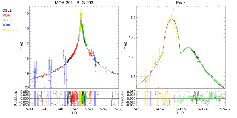
Figure 1: The light curve of MOA-2011-BLG-293. The left-hand panel shows a broad view of the light curve, while the right-hand panel highlights the peak of the event where the planetary perturbation occurs. Data from different observatories are represented by different colors, see legend. The black curve is the best-fit model with a close topology ($s<1$). The times are given in HJD^′=HJD$-2450000$.

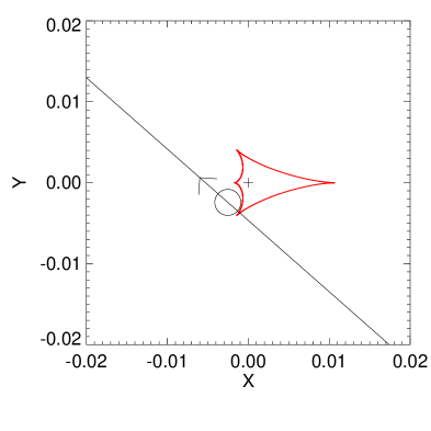
Figure 4: Caustic structure and source trajectory of the best-fit model of MOA-2011-BLG-293 in the source plane. The circle shows the physical size of the source, and its position at the time of the caustic exit ($HJD^{\prime}\sim 5747.5$). The x-axis is the star-planet axis, and the origin is at the center of magnification. The scale of the axes is in units of the Einstein radius.

The data are shown in Figure 1. Several features should be noted. First, the pronounced part of the anomaly lasts just 4 hours beginning at HJD${}^{\prime}=5747.40$. The main feature is quite striking, becoming about one magnitude brighter in about one hour. The coverage during the anomaly is temporally disjoint between the observatories in Israel and those in Chile, a point to which we return below. Finally, the CTIO data show a discontinuous change of slope (“break”), which is the hallmark of a caustic exit, when the source passes from being partially or fully inside a caustic to being fully outside the caustic (see Fig. 4).

MOA and OGLE data were reduced using their standard pipelines (Bond et al., 2001; Udalski, 2003) which are based on difference image analysis (DIA). In the case of the OGLE data, the source is undetected in the template image. Since the OGLE pipeline reports photometry in magnitudes, an artificial blend star with a flux of 800 units ($I_{OGLE}=20.44$) was added to the position of the event to prevent measurements of negative flux (and undefined magnitudes) at baseline when the source is unmagnified.

Data from the remaining three observatories were also reduced using DIA (Wozniak, 2000), with each reduction specifically adapted to that imager. Using comparison stars, the Wise and Weizmann photometry were aligned to the same flux scale as the CTIO $I$ band by inverting the technique of Gould et al. (2010b). That is, the instrumental source color was determined from CTIO observations, and then the instrumental flux ratios (CTIO vs. Wise, or CTIO vs. Weizmann) were measured for field stars of similar color. The uncertainties in these flux alignments are 0.016 mag for Wise and 0.061 mag for Weizmann.

2.1 Data Binning and Error Normalization

Since photometry packages typically underestimate the true errors, which have a contribution from systematics, we renormalize the error bars on the data, as is done for most microlensing events. After finding an initial model, we calculate the cumulative $\chi^{2}$ distribution for each set of data sorted by magnification. We renormalize the error bars using the formula

$$\sigma_{i}^{\prime}=k\sqrt{\sigma_{i}^{2}+e_{\rm min}^{2}}$$ (1)

and choosing values of $k$ and $e_{\rm min}$ such that the $\chi^{2}$ per degree of freedom $\chi^{2}_{\rm red}=1$ and the cumulative sum of $\chi^{2}$ is approximately linear as a function of source magnification. Specifically, we sort the data points by magnification, calculate the $\Delta\chi^{2}$ contributed by each point, and plot $\sum^{N}_{i}\Delta\chi^{2}_{i}$ as a function of $N$ to create the cumulative sum of $\chi^{2}$, where $N$ is the number of points with magnification less than or equal to the magnification of point $N$. Note that $\sigma_{i}$ is the uncertainty in magnitudes (rather than flux). The values of $k$ and $e_{\rm min}$ for each data set are given in Table 1. Except for OGLE, the values of $e_{\rm min}$ are all zero. This term compensates for unrealistically small uncertainties in the measured magnitude, which can happen when the event is bright and the Poisson flux errors are small.

For the MOA data, we eliminate all observations with $t$ outside the interval $5743.5<t(HJD^{\prime})<5749.5$ (see Section 4.2). We also exclude all MOA points with seeing $>5^{\prime\prime}$ because these data show a strong nonlinear trend with seeing at baseline. After making these cuts, we renormalize the data as described above.

To speed computation, the OGLE and MOA data in the wings of the event were binned. In the process of the binning, $3\sigma$ outliers were removed. This binning does not account for correlations in the data, which if they exist can increase the reduced $\chi^{2}$ above the nominal value of $\chi^{2}_{\rm red}=1$.

3 CMD

We use the CTIO $I$ and $V$ band data to construct a color-magnitude diagram (CMD) of the event. We measure the instrumental (uncalibrated) source color by linear regression of the $V$ and $I$ fluxes (which is independent of the model) and the magnitude from the $f_{S,{\rm CTIO}}$ of our best-fit model: $(V-I,I)_{S}=(0.37,22.27)\pm(0.03,0.05)$. The position of the source relative to the field stars within 60^′′ of the source (small dots) is shown in Figure 2 as the solid black dot. We calibrate these magnitudes and account for the reddening toward the field by assuming the source is in (or at least suffers the same extinction as) the Bulge and using the centroid of the red clump as a standard candle. Because of strong differential extinction across the field, we use only stars within 60^′′ of the source to measure the centroid of the red clump. Since the event is in a low latitude field, there are more stars than is typical for bulge fields and the red-clump centroid can be reliably determined even with this restriction. In instrumental magnitudes, the centroid of the red clump is $(V-I,I)_{cl}=(0.59,16.90)$ compared to its intrinsic value of $(V-I,I)_{cl,0}=(1.06,14.32)$ (Bensby et al., 2011; Nataf, 2012), which assumes a Galactocentric distance $R_{0}=8\,$kpc and that the mean clump distance toward $l=1.5$ lies 0.1 mag closer than $R_{0}$ (Rattenbury, 2007). We can apply the offset between these two values to the source color and magnitude to obtain the calibrated, dereddened values $(V-I,I)_{S,0}=(0.84,19.69)\pm(0.05,0.16)$. The uncertainty in the color is derived from Bensby et al. (2011) by comparing the spectroscopic colors to the microlens colors of that sample. The uncertainty in the calibrated magnitude is the sum in quadrature of the uncertainty in $f_{S,{\rm CTIO}}$ from the models (0.05 mag), the uncertainty in $R_{0}$ (5%$\rightarrow$0.1 mag), the uncertainty in the intrinsic clump magnitude (0.05 mag), and the uncertainty in centroiding the red clump (0.1 mag).

4 Effect of Faint Sources on Microlens Parameters

The source star in MOA-2011-BLG-293 is extremely faint with an apparent magnitude in the OGLE photometry of $I_{S,{\rm OGLE}}=21.7$. Consequently, the measured flux errors can be comparable to or larger than the source flux, particularly near baseline. Because of this, systematics in the baseline data must be carefully accounted for so as not to bias the microlens results. Systematics in the measured flux at the level of $f_{S}$ can lead to biases in the measured Einstein timescale, $t_{\rm E}$, of the same order. We begin by discussing robust parameters, which can be measured solely from the highly magnified portion of the light curve and so, are independent of uncertainties in the flux measured near baseline. Then in Section 4.2, we discuss in detail the effect of systematics in the measured baseline flux on the microlens parameters, particularly $t_{E}$ and the mass ratio between the components of the lens, $q$.

4.1 Robustly Measured Parameters

At high magnification, a microlensing light curve for a point source being lensed by a point lens can be described by the unmagnified, baseline flux of the event, $f_{\rm base}$, and three parameters (“invariants”): the time of the peak, $t_{0}$, the difference between $f_{\rm base}$ and the peak flux, $f_{\rm lim}$, and the effective width of the light curve, $t_{\rm eff}$ (Gould, 1996, see Eq. (2.4) and (2.5) in). These parameters are nearly invariant under changes to the source flux and are robustly determined by the light curve. The change in the observed flux due to the event can then be written as a function of these invariants:

$$f_{\rm obs}(t)-f_{\rm base}=G_{3}(t;t_{0},t_{\rm eff},f_{\rm lim}),$$ (2)

where $f_{\rm obs}$ is the observed flux and the subscript on $G$ refers to the number of parameters. Note that $f_{\rm base}$ is also an observable.

In the limit where the event is highly magnified, the exact form of $G_{3}(t)$ can be derived from the microlens variables. The three microlens variables of a point-source–point-lens microlensing model are $t_{0}$, the impact parameter in units of the Einstein radius, $u_{0}$, and the Einstein crossing time, $t_{\rm E}$. The observed flux is given by

$$f_{\rm obs}=f_{S}A(t)+f_{B}=f_{S}[A(t)-1]+f_{\rm base},$$ (3)

where $A(t)$ is the magnification of the source, $f_{S}$ is the flux of the source, and $f_{B}$ is the flux of all other stars blended into the PSF (including the flux from the lens). By definition, $f_{\rm base}=f_{S}+f_{B}$. For a point lens in the limit of high magnification ($A(t)\gg 1$), the magnification is given by

$$A(t)\simeq\frac{1}{u_{0}Q(t)}$$ (4)

where

$$Q(t;t_{0},t_{\rm eff})=\sqrt{1+\left(\frac{t-t_{0}}{t_{\rm eff}}\right)^{2}},$$ (5)

is a function of only time and the invariant:

$$t_{\rm eff}\equiv u_{0}t_{\rm E}.$$ (6)

In this limit, the evolution of the observed flux, $G_{3}(t;t_{0},t_{\rm eff},f_{\rm lim})$, is then given by

$$G_{3}(t;t_{0},t_{\rm eff},f_{\rm lim})=\frac{f_{\rm lim}}{Q(t)},\mathrm{\,where\,}f_{\rm lim}\equiv\frac{f_{S}}{u_{0}}.$$ (7)

If finite source effects are detected, the change in the observed flux is a more complicated function because of the additional microlens parameter $\rho$, which is the source size in units of the Einstein radius. However, there is also an additional invariant

$$t_{\star}\equiv\rho t_{E},$$ (8)

the source crossing time, which determines the width of the peak of the light curve for a point lens. Hence, the change in the observed flux can be written as

$$f_{\rm obs}(t)-f_{\rm base}=G_{4}(t;t_{0},t_{\rm eff},f_{\rm lim},t_{\star})=G_{3}(t)B\left(Qt_{\rm eff}/t_{\star}\right),$$ (9)

where $B(Qt_{\rm eff}/t_{\star})=B(u/\rho)$ is a function composed of elliptic integrals, whose exact form is derived in Gould (1994) and Yoo et al. (2004).

In the case of a two-body lens like MOA-2011-BLG-293, the invariants may not be obvious from the light curve, but they are still robustly measured as we show below. For example, the width of the peak is distorted by two-body perturbation, but based on the source trajectory (Fig. 4), it can be seen that the width of the first bump at HJD${}^{\prime}5747.46$, which is caused by the cusp crossing, will be slightly larger than $2t_{\star}$. For a two-body lens with a central caustic crossing, there is also another invariant due to the mass ratio, $q$, between the two lensing bodies, so

$$f_{\rm obs}(t)-f_{\rm base}=G_{5}(t;t_{0},t_{\rm eff},f_{\rm lim},t_{\star},qt_{E}).$$ (10)

This new invariant $qt_{\rm E}$ can be understood as follows. For central caustics, like the one in MOA-2011-BLG-293, the caustic size is proportional to the mass ratio of the two lensing bodies, $q$, and the caustic shape is roughly constant for a given $s$. Therefore, the time between successive features in the light curve is set by $qt_{\rm E}$, i.e., the size of the caustic multiplied by the characteristic timescale, and since the observed times of the features can be well measured, the uncertainty in this quantity is extremely small. In this case, the main features are the two bumps in the light curve and the discontinuity in the slope that occurs between the bumps. [Note that a two-body lens introduces two parameters in addition to $q$: the separation between the two bodies projected onto the plane of the sky, $s$, and the angle of the source trajectory with respect to the binary axis, $\alpha$. Because these parameters are of less interest, we do not discuss them in this context.]

Table 2 shows that for this event these quantities, $t_{\rm eff}$, $f_{\rm lim}$, $t_{\star}$, and $qt_{\rm E}$, do indeed have extremely small uncertainties and can approximately be considered invariants.

4.2 Parameters Vulnerable to Systematics

The above invariants are determined by the data taken near the peak of the light curve where $A\gg 1$. However, in order to extract the values of the microlens parameters, $u_{0}$, $\rho$, and $q$, from the invariants, we must measure $t_{\rm E}$. The information on $t_{E}$ must necessarily come from the wings of the light curve where the magnification is small and $A(t)\neq 1/u(t)$ (Dominik, 2009). Since the magnification is small, the change in the observed flux compared to the source flux is also small, so the measurement of $t_{E}$ may be considered to be the statistical sum of many measurements of a small change in flux. In order to get an accurate measurement of $t_{\rm E}$, the statistical and systematic errors in the flux must be smaller than the change we are trying to measure.

In the case of MOA-2011-BLG-293, because the source flux is extremely faint, it is difficult to measure accurately. When the magnification is a factor of a few or less (in the wings and at baseline), if the flux is not measured with an accuracy substantially smaller than the source flux, this can lead to bias in the measurement of $f_{S}$ or equivalently $t_{\rm E}$, since $f_{S}t_{\rm E}=f_{\rm lim}t_{\rm eff}$ is robustly determined, and so to bias in quantities dependent on $t_{\rm E}$ such as $q$. To check for this possible source of bias, we bin the OGLE and MOA data by 30 days to see if their measurements of the baseline flux are stable (Fig. 3). We find that the OGLE measurement of the baseline flux is stable at a level that is smaller than the observed source flux. Therefore, we use all of the OGLE data in our models. We note that the flux after the event ($t>{\rm HJD}^{\prime}5790$) appears to be at a lower level than the baseline before the event. In Section 5.1, we discuss the effect of assuming the baseline decreases at a constant rate during the course of the event.

As seen in Figure 3, the MOA baseline flux exhibits scatter in excess of the measured photometric errors, and there is also variation in measured baseline flux from season to season. The magnitude of this scatter is similar to the magnitude of the source flux. Because of this variation, we conclude that the baseline flux is not sufficiently well measured in the MOA data to detect the small changes in flux necessary to measure $t_{E}$. As a result, to avoid biasing our results, we use only the MOA data from the peak of the light curve where the photometry is precise: $5743.5<t({\rm HJD}^{\prime})<5749.5$.

5 Analysis

Without any modeling, we can make some basic inferences about the relevant microlens parameters from inspection of the light curve. MOA-2011-BLG-293 increases in brightness from $I\sim 19.7$ to $I\sim 15.0$, indicating a source magnification of at least 75. Additionally, except for the deviations at the peak, the event is symmetric about $t_{0}$. From these two properties, we infer that only central or resonant caustics (both of which are centered on the position of the primary) are relevant to the search for microlens models.

We fit the light curve using a Markov Chain Monte Carlo (MCMC) procedure. In addition to the parameters described in Section 4, a model with a two-body lens has two additional parameters: the angle of the source trajectory with respect to the binary axis defined to be positive in the clockwise direction, $\alpha$, and the projected separation between the two components of the lens scaled to the Einstein radius, $s$. Because they are approximately constants, we use the parameters $t_{\rm eff}$ and $t_{\star}$ in place of the microlens variables $u_{0}$ and $\rho$. For a given model, Equation (3) must be evaluated for each observatory, $i$, so $f_{S},f_{B}\rightarrow f_{S,i},f_{B,i}$. We adopt the “natural” linear limb-darkening coefficients $\Gamma=2u/(3-u)$ (Albrow et al., 1999). Based on the measured position of the source in the CMD, we estimate that $T_{\rm eff}=5315$K and $\log g=4.5$ cgs. We average the linear limb-darkening coefficients for $T_{\rm eff}=5250$K and $T_{\rm eff}=5500$K from Claret (2000) assuming $v_{\rm turb}=2\,$km s^-1 to find $\Gamma_{V}=0.6368$ and $\Gamma_{I}=0.4602$.

The magnifications are calculated on an $(s,q)$ grid, using the “map-making” technique (Dong et al., 2006) in the strong finite-source regime and the “hexadecapole” approximation (Pejcha & Heyrovský, 2009; Gould, 2008) in the intermediate regime.

We began by searching a grid of $s$ and $q$ to obtain a basic solution for the light curve. For central caustic crossing events like this one, there is a well known degeneracy between models with close topologies ($s<1$) and wide topologies ($s>1$) (e.g. Griest & Safizadeh, 1998). We initially searched a broad grid for close topologies and then used the results to inform our search for wide solutions, since to first order, $s\rightarrow s^{-1}$. The basic model from this broad grid has $s\sim 0.55$, $q\sim 0.005$, and $\alpha\sim 220^{\circ}$, such that the source passes over a cusp at the back end of a central caustic. This caustic is created by a two-body lens with a mass ratio similar to that of a massive Jovian planet orbiting a star. Figure 4 shows this basic geometry with the source trajectory relative to the caustic structure. The bump in the light curve at HJD${}^{\prime}\sim 5747.45$ is created when the source passes over the cusp of the caustic.

Because the Wise and Weizmann data only overlap with other data sets where their errors are extremely large, there is some concern that the parameters of the models will be poorly constrained, since within the standard modeling approach the flux levels of these data can be arbitrarily adjusted up or down relative to the other data. However, from the flux alignment described in Section 2, we have an estimate of $f_{S,i}$ for these data relative to $f_{S,{\rm CTIO}}$. This alignment gives us an independent means to test the validity of our model. If the model is correct, then the values of $f_{S,{\rm Wise}}$ and $f_{S,{\rm Weizmann}}$ should agree with $f_{S,{\rm CTIO}}$ within the allowed uncertainties. Alternatively, if we include the flux-alignment constraint in the MCMC fits, the solution should not change significantly.

We incorporate the flux-alignment constraint in a way that is parallel to the model constraints from the data, i.e., by introducing a $\chi^{2}$ penalty:

$$\chi^{2}_{b}=\sum_{i}\frac{(f_{S,{\rm CTIO}}-f_{S,i})^{2}}{\sigma_{{\rm flux},i}^{2}};\quad\sigma_{{\rm flux},i}=\frac{\ln 10}{2.5}\left(\frac{f_{S,{\rm CTIO}}+f_{S,i}}{2}\right)\sigma_{i},$$ (11)

where $i$ corresponds to the observatory with the constraint, and $\sigma_{i}$ is the uncertainty in magnitudes of the flux alignment for that observatory. In the absence of any constraints, the flux parameters for each observatory, $f_{S,i}$ and $f_{B,i}$, are linear and their values for a particular model can be found by inverting a block-diagonal covariance matrix, $b$. We include the flux constraints by adding half of the second derivatives of $\chi^{2}_{b}$ to the $b$ matrix:

$$\Delta b(f_{S,i},f_{S,k})={2\delta_{ik}-1\over\sigma_{{\rm flux},i}^{2}},$$ (12)

where $k=$CTIO and $\delta_{ik}$ is a Kronecker-delta. This couples formerly independent $2\times 2$ blocks. Strictly speaking, the equation for $\sigma_{{\rm flux},i}$ given in Equation (11) is a numerical approximation. Therefore, we iterate the linear fit until the value of $\sigma_{{\rm flux},i}$ is converged, which typically occurs in only a few iterations.

We refined the $(s,q)$ grid around our initial close solution, fitting the data both with and without flux-alignment constraints. The mean and $1\,\sigma$ confidence intervals for the parameters from these two fits are given in Table 3. There are only small quantitative differences between the two solutions, and nothing that changes the qualitative behavior of the model. The slight increase in $\chi^{2}$ is expected because of the additional term due to the flux constraints. After finding this close solution, we repeated the grid with $s\rightarrow s^{-1}$ to identify the wide solution. The parameters of this solution are also given in Table 3 both with and without flux-alignment constraints. The close solution is mildly preferred over the wide solution by $\Delta\chi^{2}\sim 3$, so we quote the values for the flux-constrained close solution:

$$q=5.3\pm 0.2\times 10^{-3}\qquad s=0.548\pm 0.005,$$ (13)

noting that the two topologies give very similar solutions (except $s\rightarrow s^{-1}$).

Additionally, we searched for a parallax signal in the event by adding two additional free parameters to the fit for the close solution: $\pi_{{\rm E},N}$ and $\pi_{{\rm E},E}$, the North and East components of the parallax vector (e.g., Gould 2004). The parameters of this fit are given in Table 3. No parallax signal was detected, and we found no interesting constraints on these parameters. The $\chi^{2}$ improves for fits including parallax by only $\Delta\chi^{2}=7$ for two additional degrees of freedom. In some cases, even when parallax is not detected, meaningful upper limits can be placed on the parallax, but in this case we have an uninteresting 3$\sigma$ constraint of $0\leq|\pi_{\rm E}|\leq 7.8$.

5.1 Effect of Systematics in $f_{\rm base}$

As discussed in Section 4.2, it is possible that the underlying OGLE baseline flux is changing during the course of the event. In order to test how that could introduce systematic effects in our results, we create a fake OGLE data set accounting for a constant decrease in baseline flux during the event. Specifically, we assume that the baseline flux decreases at a constant rate between HJD${}^{\prime}5710.$ and HJD${}^{\prime}5790.$ leading to an overall decrease in flux of $0.27f_{S,{\rm OGLE}}$. We then repeat the MCMC procedure for the close solution including flux-alignment constraints. We find that the value of $t_{E}$ increases by 15%, and consequently, the values of $q$, $u_{0}$, and $\rho$ decrease by the same amount. In principle, this could represent a systematic error in our results. However, at the present time, the evidence for a change in the baseline flux is weak, so we only report these results for the sake of completeness.

5.2 Analysis with Survey-Only Data

From this analysis, we have a robustly detected planet ($\Delta\chi^{2}\sim 5400$ compared to a point lens) and a well-defined solution. Now we can ask whether the planet could have been detected from the survey data alone, whether the solution is well-constrained, and most importantly, whether it is the same solution. To begin, we construct a “survey only” subset of the data. We first eliminate the Weizmann and CTIO data. Second, we “thin out” the OGLE data to mimic OGLE survey data as they would have been if there had been no high-magnification or anomaly alerts. OGLE data on several nights previous to (and following) the peak have a cadence of 1 observation per 0.015 days. We therefore adopt a subset of 18 (out of 44) OGLE points from the peak night with this sampling rate.

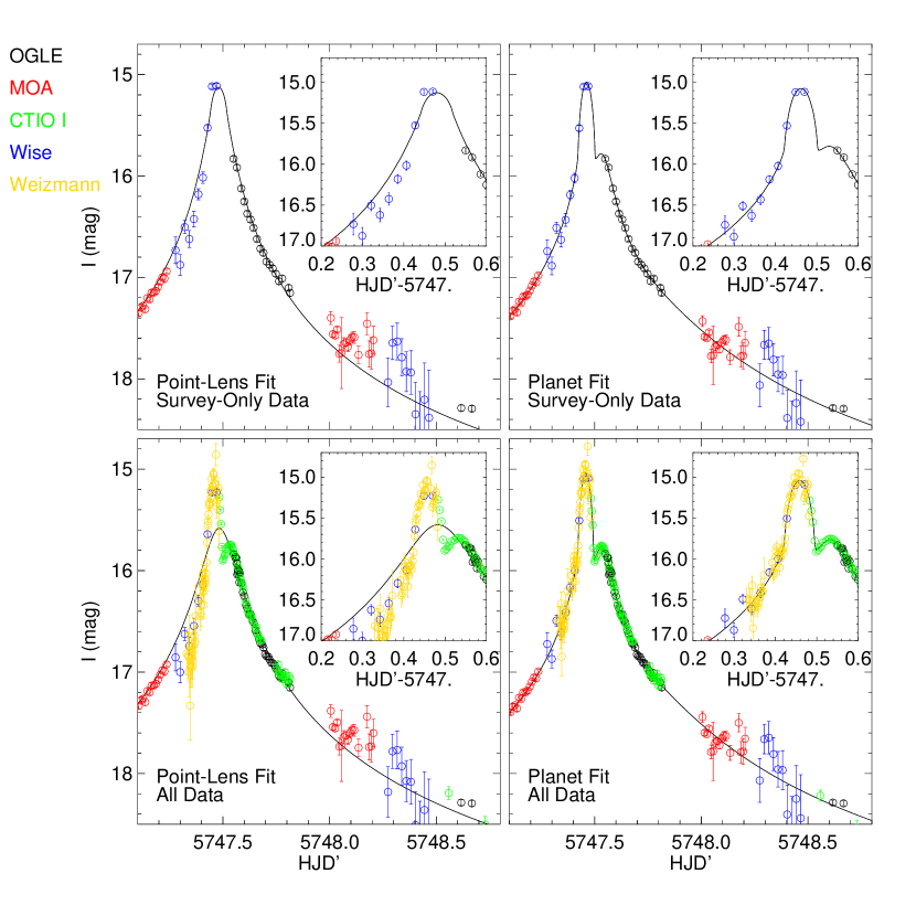
Figure 5: Comparison of point-lens fits (left) and planet fits (right) for “survey-only” data, (top) and all data (bottom). In both cases, the planet fit is clearly better than the point lens fit, but the difference is more significant when followup data are included. Note that for “survey-only” data the OGLE data have been thinned out to reflect the typical survey cadence.

We repeat the analysis on this survey-only data set beginning with a broad grid search and then refining the solution following the same procedure used for analyzing the complete data set. We find that even without flux-alignment constraints, the global search isolates solutions in the general neighborhood of the solution found from the full data set. The fits to the survey-only data set are compared to fits with all data in Figure 5. Here, the $\Delta\chi^{2}$ of the fit compared to a point lens fit for the survey-only data is 487, nearly all of which comes from data in the time-span shown in Figure 5 $5747.1<t(HJD^{\prime})<5748.8$. This is smaller than the $\Delta\chi^{2}$ of any published microlensing planet. However, the parameters of the fit are well constrained with errors only a factor of 1.5-2 larger compared to fits with the full data set. Applying the flux-alignment constraint to this model confirms its validity, i.e., it does not appreciably change the solution (see Table 3). In this case, it is clear that the survey data are sufficient to robustly detect and characterize the planet.

In order to push farther into the limits of detectability, we also analyze this event without the Wise data, since those data contain most of the deviation from the underlying point lens. With only the MOA and thinned OGLE data, we find $\Delta\chi^{2}\sim 70$ between the 2-body lens and point lens models. We note that the point lens model has an unreasonably large value of parallax, $\pi_{\rm E}\sim 20$, making it somewhat suspicious. Without parallax, the $\Delta\chi^{2}$ between the point lens and 2-body fit increases to $\Delta\chi^{2}\sim 170$. Although this is a factor of 3 smaller than the $\Delta\chi^{2}$ with the Wise data, the constraints on the planet-star mass ratio are still broadly confined to be planetary, assuming $M_{L}\lesssim 0.5$M_⊙, with a $3\sigma$ range of $0.001\lesssim q\lesssim 0.025$. However, because of the small $\Delta\chi^{2}$, it appears unlikely to us that a planetary detection would have been claimed from solely the MOA and OGLE data even though the solution is formally well-constrained.

6 Physical Properties of the Event

Since finite source effects are measured in this event, we can determine the angular size of the Einstein ring, $\theta_{\rm E}$, and the lens-source relative proper motion, $\mu$. First, we estimate the angular size of the source, $\theta_{\star}$, from the observed color and magnitude. We transform the $(V-I)_{S,0}$ color to $(V-K)$ using the dwarf relation from Bessell & Brett (1988). Then we use the $(V-K)$ surface brightness relations from Kervella et al. (2004) to find $\theta_{\star}=0.42\pm 0.03\,\mu$as. From this we derive the lens-source relative proper motion and angular Einstein radius,

$$\mu=\frac{\theta_{\star}}{t_{\star}}=4.3\pm 0.3\,{\rm mas\,yr^{-1}};\quad\theta_{\rm E}=\mu t_{\rm E}=0.26\pm 0.02\,{\rm mas}.$$ (14)

The uncertainties in these quantities come from a variety of factors. Specifically, the uncertainties in the Galactocentric distance, $R_{0}$, and the measured intrinsic brightness of the red clump, the centroiding of the red clump from the CMD, and uncertainty in the surface brightness relations. The uncertainty contributed by the surface brightness relations is 0.02 mag, and the uncertainties from the other factors are given in Section 3. The contribution of these factors can be understood from their relationship to $\theta_{\star}$ (Yee et al., 2009):

$$\theta_{\star}=\frac{\sqrt{f_{S}}}{Z},$$ (15)

where $f_{S}$ is the source flux from the microlensing model and $Z$ captures all other factors. Taking account of all factors mentioned above, we find $\sigma(Z)/Z=8\%$. Since the statistical error in $f_{S}^{1/2}$ is only 2.3%, the error in $Z$ completely dominates the uncertainty in $\theta_{*}$. In general, the error in $f_{S}$ propagates in opposite directions for $\theta_{\rm E}$ and $\mu$ (Yee et al., 2009). However, in the present case, since this error is small, the fractional error in these quantities is simply that of $Z$, as indicated in Equation (14).

7 Properties of the Lens

7.1 Limits on the Lens Brightness

We can use the observed brightness of the event to place constraints on the lens mass. Since the source and lens are superposed, any light from the lens should be accounted for by the blend flux, $f_{B,i}$, which sets an upper limit on the light from the lens. The unmagnified source is not seen in the OGLE data. From examination of an OGLE image at baseline with good seeing, we estimate the upper limit of the blend flux to be $I_{B,0}\geq 17.77$ based on the diffuse background light and assuming that the reddening is the same as the red clump. Assuming all of this light is due to the lens, the absolute magnitude of the lens is

$$M_{I,L}>I_{B,0}+(A_{I,S}-A_{I,L})-5\log{D_{L}\over 10\,{\rm pc}}=3.25+(A_{I,S}-A_{I,L})+5\log{R_{0}\over D_{L}},$$ (16)

where $A_{I,S}$ and $A_{I,L}$ are the reddening toward the source and lens, respectively, and $D_{L}$ is the distance to the lens. Since the lens must be in front of the source, we have $A_{I,S}\geq A_{I,L}$. Moreover, the lens should be closer than $R_{0}$ (or at any rate, not much farther). Hence, $M_{I,L}\geq 3.25$ is a conservative lower limit. From the empirical isochrones of An et al. (2007), this absolute magnitude corresponds to an upper limit in the lens mass of $M_{L}\leq 1.2M_{\odot}$. We conclude from these flux-alignment constraints that either the lens is a main sequence star or, if it is more massive than our upper limit of $1.2M_{\odot}$, then it must be a stellar remnant such as a very massive white dwarf or a neutron star.

We can use our measurement of $\theta_{\rm E}$ to estimate the distance to the lens based on its mass:

$$D_{L}=\left(\frac{\theta_{\rm E}^{2}}{\kappa M_{L}}\frac{1}{\rm AU}+\frac{1}{D_{S}}\right)^{-1}\mathrm{\,with\,}\kappa\equiv\frac{4G}{c^{2}\mathrm{AU}}=8.14\mathrm{\,mas\,}M_{\odot}^{-1},$$ (17)

where $D_{S}$ is the distance to the source. If we assume the source is at 8 kpc (i.e., about 0.1 mag behind the mean distance to the clump at this location) and $M_{L}=1.2M_{\odot}$, we find $D_{L}=7.6\,$kpc. Hence, the lens could be an F/G dwarf or stellar remnant in the Bulge, or it could be a late-type star closer to the Sun.

7.2 Bayesian Analysis

Similar to Alcock et al. (1997) and Dominik (2006), we estimate the mass of the lens star and its distance using Bayesian analysis accounting for the measured microlensing parameters, the brightness constraints on the lens, and a model for the Galaxy. The mathematics are similar to what is described in Section 5 of Batista et al. (2011), although the implementation is fundamentally different because we do not have meaningful parallax information. Specifically, we perform a numerical integral instead of applying the Bayesian analysis to the results of the MCMC procedure. We begin with the rate equation for lensing events:

$$\frac{d^{4}\Gamma}{dD_{L}dM_{L}d^{2}\mu}=\nu(x,y,z)(2R_{\rm E})v_{\rm rel}f({\bf\mu})g(M_{L}),$$ (18)

where $\nu(x,y,z)$ is the density of lenses, $R_{\rm E}$ is the physical Einstein radius, $v_{\rm rel}$ is the lens-source relative velocity, $f({\bf\mu})$ is the weighting for the lens-source relative proper motion, and $g(M_{L})$ is the mass function. The vector form of the lens-source relative proper motion is $\mu$, which can be described by a magnitude, $\mu$, and an angle, $\phi$, such that $d^{2}\mu=\mu d\mu d\phi$. We transform variables (see Batista et al. 2011) to find

$$\frac{d^{4}\Gamma}{dD_{L}d\theta_{\rm E}dt_{\rm E}d\phi}=\frac{2D_{L}^{2}\mu^{4}\theta_{\rm E}}{\kappa\pi_{\rm rel}}\nu(x,y,z)f({\mbox{\boldmath$\mu$}})g(M_{L}).$$ (19)

To find the probability density functions for the lens, we integrate this equation over the variables $\theta_{E}$ and $\phi$, using a Gaussian prior for $\theta_{E}$ with the values given in Eq. (14) and a flat prior for $\phi$. We calculate $\mu$ from $t_{\rm E}$ and $\theta_{\rm E}$ using Equation (14). We also integrate over $D_{S}$, which appears implicitly in $\pi_{\rm rel}$ and $f(\mu)$. For $D_{S}$, we include a prior for the density of sources based on our Galactic model (see below) assuming the source is in the Bulge.

Three functions remain to be defined: $\nu(x,y,z)$, $f({\mbox{\boldmath$\mu$}})$, and $g(M_{L})$. As in Batista et al. (2011), we assume $g(M)\propto M^{-1}$. For the proper motion term, we follow Equation (19) of Batista et al. (2011):

$$f_{\mu}\propto\frac{1}{\sigma_{\mu,{N_{\rm gal}}}\sigma_{\mu,E_{\rm gal}}}\exp{\left[-\frac{(\mu_{N_{\rm gal}}-\mu_{{\rm exp},N_{\rm gal}})^{2}}{2\sigma_{\mu,N_{\rm gal}}^{2}}-\frac{(\mu_{\rm E_{\rm gal}}-\mu_{{\rm exp},E_{\rm gal}})^{2}}{2\sigma_{\mu,E_{\rm gal}}^{2}}\right]}.$$ (20)

Note that the variables in $f_{\mu}$ are given in Galactic coordinates rather than Equatorial coordinates. The transformation between the two is simply a rotation by 60^∘. Still working in Galactic coordinates, the expected proper motion, ${\mbox{\boldmath$\mu$}}_{\rm exp}$, takes into account the typical motion of a star in the Disk, ${\bf v}$, and the motion of the Earth during the event, ${\bf v}_{\oplus}=(v_{\oplus,N_{\rm gal}},v_{\oplus,E_{\rm gal}})=(-0.80,28.52)\,\mathrm{km\,s^{-1}}$,

$${\mbox{\boldmath$\mu$}}_{\rm exp}=\frac{{\bf v}_{L}-({\bf v}_{\odot}+{\bf v}_{\oplus})}{D_{L}}-\frac{{\bf v}_{S}-({\bf v}_{\odot}+{\bf v}_{\oplus})}{D_{S}},$$ (21)

where ${\bf v}_{\odot}=(7,12)\,{\rm km}\,{\rm s}^{-1}+(0,v_{\rm rot})$ and $v_{\rm rot}=230\,{\rm km}\,{\rm s}^{-1}$. For the Disk we use ${\bf v}=(0,v_{\rm rot}-10\,\mathrm{km\,s^{-1}})$ and ${\mbox{\boldmath$\sigma$}}=(\sigma_{\mu,N_{\rm gal}},\sigma_{\mu,E_{\rm gal}})=(20,30)\,\mathrm{km\,s^{-1}}$, and for the Bulge ${\bf v}=(0,0)\,\mathrm{km\,s^{-1}}$ and ${\mbox{\boldmath$\sigma$}}=(\sigma_{\mu,N_{\rm gal}},\sigma_{\mu,E_{\rm gal}})=(100,100)\,\mathrm{km\,s^{-1}}$.

For the stellar density $\nu(x,y,z)$, we use the model from Han & Gould (2003) including a bar in the Bulge. We assume the Disk has cylindrical symmetry with a hole of radius 1 kpc centered at $R_{0}=8\,$ kpc. We limit the Bulge to $5<D<10\,$ kpc, where $D$ is the distance from the observer along the line of sight.

For the Bayesian analysis, we use $t_{E}=21.7$ days measured from the microlensing fit to the light curve. We also have the constraint from the lens brightness that $M_{L}=\theta_{E}^{2}/(\kappa\pi_{\rm rel})<1.2M_{\odot}$. This analysis implicitly assumes that the lens is a main sequence star. The lens could be a stellar remnant, although this is much less likely because of their smaller relative space density. The possibility that the lens is a stellar remnant could be tested several years from now when the source and lens have moved sufficiently far apart so as to be separately resolved, i.e., in roughly $10(\lambda/1.6{\rm\mu m})(D_{\rm tel}/10{\rm m})^{-1}$ years, where $\lambda$ is the wavelength of the observations and $D_{\rm tel}$ is the diameter of the telescope used, assuming the observations are diffraction limited (for a discussion of detecting light from a main sequence lens, see the Appendix).

The results of the Bayesian analysis are shown in Figure 6. We find that if the lens is a main sequence star, its mass is $M_{L}=0.43^{+0.27}_{-0.17}\,M_{\odot}$ and its distance is $D_{L}=7.15\pm 0.75\,$kpc (median and 68% confidence interval). Hence the planet mass is $m_{p}=2.4^{+1.5}_{-0.9}\,M_{\rm Jup}$. In the close solution, the projected separation is sharply peaked at $r_{\perp}=sD_{L}\theta_{\rm E}=\,1.0\pm 0.1\,$AU. However, the wide solution, which is not strongly disfavored, gives an alternative $r_{\perp}=3.4\pm 0.4\,$AU. If we assume $a\sim r_{\perp}$, the planet would have a period of $\sim 1.5$ or $\sim 8$ years.

8 Discussion

8.1 Implications for Planet Formation Theory

The lens in MOA-2011-BLG-293 consists of a super-Jupiter orbiting a probable M dwarf. The projected separation of the planet from the star is at most a few AU, making it difficult to form in situ if the host is indeed an M dwarf. Core accretion theory makes a general prediction that massive Jovian planets around M dwarfs should be rare (Laughlin et al., 2004; Ida & Lin, 2005). While gravitational instability can form large planets around M dwarfs (Boss, 2006), these typically form farther out, so if the planet formed by this mechanism, it would either be required to have migrated significantly or the projection effects must be severe. In the Appendix, we discuss how Adaptive Optics (AO) observations can confirm the microlensing measurement of the host mass or at least place upper limits on the host mass that would confine it to the M dwarf regime. Additionally, it should be noted that this planet joins a growing number of massive planets orbiting stars likely to be M dwarfs discovered by microlensing (see Appendix) and radial velocity (see Bonfils et al. 2011 for a summary and also Johnson et al. 2011).

8.2 The Ongoing Importance of Followup

Even with high-cadence surveys, followup data remain important for the interpretation of individual events. In this case, the event was high magnification with a faint source, undetected at baseline. This meant that the time period when the event was observable, to surveys and followup, was very brief. We have shown that followup data can vastly increase the signal and provide redundancy in the light curve coverage, which protects against weather. In Section 5.2, we demonstrated that with the survey data, even though the break in the light curve is missed because of bad weather, the same solution is recovered for MOA-2011-BLG-293, albeit at much lower significance than when all the data are included ($\Delta\chi^{2}\sim 500$ compared to $\Delta\chi^{2}\sim 5400$). This is somewhat surprising since it is conceivable that because of the degeneracies possible for central caustic type events, the loss of this feature would leave the models relatively unconstrained or allow alternative solutions to the light curve. The followup data are beneficial in this case because in addition to adding to the signal-to-noise, they trace the sharp feature seen in the model light curves, increasing our confidence that the correct model has been found.

It is likely that without the real-time discovery of this event in the MOA data and the subsequent high magnification alert from $\mu$FUN, the planet would have remained undiscovered as of this writing. The planetary anomaly only becomes detectable when data from all three survey telescopes are combined, which requires systematically reducing, combining, and searching all of the survey data, preferably using a difference imaging reduction in order to detect events with faint sources like this one. Routine reduction of all survey data is planned for the current OGLE/MOA/Wise survey, but has not yet been fully implemented.

The multi-band data taken by followup groups can also be important for interpreting microlensing events. In order to determine the physical characteristics of the lens from the microlens variables, we used the $(V-I)$ color of the source to estimate its angular size, thus providing a physical scale for the lens system. We also used the $(V-I)$ color to inform our choice of limb-darkening coefficients for our model. Additionally, $H$-band data are important for comparison to AO observations that may be used to improve constraints on the lens mass as discussed for this event in the Appendix. $H$-band data are routinely taken as part of followup observations at CTIO but not part of the planned surveys. The OGLE survey regularly takes $V$-band data every few days when the weather is good, and the Wise survey is planning similar observations for future seasons. Provided the event timescale is long, this will result in several points taken when the source is substantially magnified.

For the present case, the highly magnified part of the event is brief, and OGLE only obtained one $V$ band point over peak, which was taken deliberately as part of followup observations. Because the $V$-band data were only taken as part of followup, we need to consider the effect of excluding these data in the context of a pure survey detection. In principle, the $(V-I)$ color could be estimated following the method in Gould et al. (2010b), which takes advantage of the difference in the OGLE and MOA bandpasses to estimate the $(V-I)$ color from $R_{\rm MOA}-I_{\rm OGLE}$. For this event, the uncertainty of this measurement from the fits to survey-only data is $\sigma_{R-I}=0.01$ leading to a $(V-I)$ uncertainty of $\sigma_{V-I}=0.04$. In this case, the precision is not much worse than what we found from the standard technique using CTIO $V$- and $I$-band photometry, so the lack of survey $V$-band data would not have a major effect.

Finally, although this event clearly shows that a planet is detected at $\Delta\chi^{2}\sim 500$ without followup data, this is smaller than the $\Delta\chi^{2}$ of any published microlensing planet, underlining the fact that low-significance signals have not been systematically explored. Events like MOA-2011-BLG-293 that are robustly characterized with followup data but with weaker signals in the survey data can be used to probe lower $\Delta\chi^{2}$ signals and inform our understanding of the limits of what is detectable. For example, if we analyze a large number of events with a range of signal strengths in the survey data, we could determine a $\Delta\chi^{2}$ threshold for which a known signal, seen in the complete data set including followup, can no longer be distinguised from the noise. Additionally, the results for central caustic events will help us understand a $\Delta\chi^{2}$ threshold below which the model degeneracies mean that the “correct” solution, as determined from the complete data set, can no longer be recovered. We might also require that these events can be well-characterized, i.e., that degenerate central caustic models can be sufficiently disentangled so that the mass ratio is well-constrained. Understanding these thresholds will be important for analyzing large samples of events to study the planets as a population rather than individual discoveries. By analyzing a large sample of events similar to MOA-2011-BLG-293, we can empirically determine appropriate $\Delta\chi^{2}$ thresholds or investigate other statistics for both detecting planets in all microlensing events and characterizing them in central caustic events.

Appendix A Appendix: Possible Constraints from AO Observations

Of the 13 previously published microlensing planets, two are very likely to be super-Jupiters orbiting M dwarfs. In both cases, high-resolution imaging from space or the ground was needed to complete these determinations. OGLE-2005-BLG-071 has a mass ratio, $q=7.4\pm 0.4\times 10^{-3}$ (Udalski et al., 2005; Dong et al., 2009a), similar to that of MOA-2011-BLG-293 analyzed here. Dong et al. (2009a) subsequently combined Hubble Space Telescope (HST) and light curve data to determine the host mass $M_{L}=0.46\pm 0.04\,M_{\odot}$, implying that this was an $m_{p}\sim 3.5\,M_{\rm Jup}$ planet orbiting an M dwarf. Batista et al. (2011) found an even higher mass ratio for MOA-2009-BLG-387 of $q=0.0132\pm 0.003$. Their marginal detection or upper limit on the lens flux from 8m-class adaptive optics (AO) observations allowed them to place an upper limit $M<0.5\,M_{\odot}$ (90% confidence) on the host, with a median estimate of $M_{L}=0.19\,M_{\odot}$, and so $m_{p}=2.6\,M_{\rm Jup}$.

Based on our Bayesian analysis (Section 7.2), it is likely that MOA-2011-BLG-293L is another case of a super-Jupiter orbiting an M dwarf. As we now show, 8m-class adaptive optics (AO) observations could clarify the nature of the system. The main uncertainty in an AO measurement of the lens flux is the uncertainty in the source flux, since the two objects are superposed unless many years have passed since the event. Because an alternate model for the baseline flux exists in which the flux is not constant (see Section 4.2), we cannot be certain it is possible to reliably measure the blended flux. Nevertheless, for the sake of argument, we are going to assume that the baseline flux is stable, so the uncertainty in $f_{S}$ is dominated by the statistical errors from the MCMC procedure. This assumption can be tested after OGLE-IV has collected several more years of baseline data on the event. If these data confirm that the baseline is stable, the calculations in this section are applicable. If not, the limits estimated here are overly optimistic.

As mentioned in Section 6, the statistical error in $f_{S}$ is 4.6%, which is due primarily to correlations of the source flux with other model parameters, rather than errors from fitting the light curve to an individual model. Thus, the $H$-band flux (in units of the instrumental scale of CTIO $H$-band images) is known to essentially the same precision. Using standard techniques (Janczak et al., 2010; Batista et al., 2011), this flux scale can be aligned to the AO flux scale to a few percent. Hence, the AO source flux $f_{H,S}$ can be known to about 7%. This means that excess light due to the lens can be securely detected at the $3\,\sigma$ level, provided that $\Delta H\equiv H_{L}-H_{S}<1.7$ mag. This quantity can be related to the physical properties of the lens and source by

$$\Delta H\equiv H_{L}-H_{S}=\Delta M_{H}+\Delta A_{H}+\Delta{\rm Dmod}$$ (A1)

where $\Delta M_{H}\equiv M_{H,L}-M_{H,S}$, $\Delta A_{H}\equiv A_{H,L}-A_{H,S}$, and $\Delta{\rm Dmod}\equiv 5\log(D_{L}/D_{S})$. Now, in the regime we will be considering, it is very likely that $\Delta A_{H}=0$, but in any case $\Delta A_{H}\leq 0$, since the lens is in front of the source. Hence, we can conservatively ignore this term. The last term is

$$\Delta{\rm Dmod}=-5\log\biggl{(}1+{D_{S}\over{\rm AU}}{\theta_{\rm E}^{2}\over\kappa M_{L}}\biggr{)}\rightarrow-0.3{D_{S}\over 8\,{\rm kpc}}\,{0.45\,M_{\odot}\over M_{L}}$$ (A2)

where in the second step we have inserted Equation (14) and kept only the first term of the Taylor expansion of the logarithm. Hence, the lens will be detectable provided

$$M_{H,L}\lesssim M_{H,S}+2.0,$$ (A3)

where $2.0=(\Delta H-\Delta{\rm Dmod})$ assuming $D_{S}=8\,$kpc and $M_{L}=0.45\,M_{\odot}$. From its color and magnitude, the source is a late G/early K Bulge dwarf, so $M_{H,S}\sim 4.2$. Hence, all dwarfs $M_{H,L}\lesssim 6.2$ are detectable, which corresponds to $M_{L}\gtrsim 0.43\,M_{\odot}$.

Such a detection or upper limit would not be absolutely secure. Detected light could in principle be due to a companion to the lens or source, or an unrelated star in this crowded, low-latitude Bulge field. Additionally, an upper limit on the lens flux could be attributed to a remnant host rather than a late M dwarf. Nevertheless, the probabilities of these alternative interpretations can be quantified, and it is important to do so in order to estimate the frequency of very massive planets orbiting M dwarfs.

Figure 2: Color-Magnitude Diagram of the event in instrumental (uncalibrated) magnitudes. The source is shown as the solid black point; the errors in the source color and magnitude are smaller than the size of the point. The centroid of the Red Clump is the open square with an X through it. The small points show the stars in the field, restricted to stars within 60^′′ of the source because there is strong differential reddening on larger scales.

Figure 3: Observed MOA (open squares) and OGLE (solid circles) fluxes at baseline. The fluxes have been scaled by the source flux and adjusted so that the baseline is approximately zero. The solid line shows the expected flux from the model. The data have been binned by 30 days (right panel) and semi-annually (left panel). Data taken when the event is significantly magnified (hashed region: $5710<t(HJD^{\prime})<5790$) have been excluded. Note that the MOA data show significant variation at a level comparable to the source flux.

Figure 6: Probability densities for the lens (host) as function of its distance (top) and mass (bottom). The vertical scale is set so that the total area under each curve is equal to one. Masses $M_{L}>1.2\,M_{\odot}$ are excluded by the flux-alignment constraint on the lens brightness (bold vertical line). The 68% and 90% confidence intervals about the median are indicated by the shaded regions. The discontinuities in the slope of probability distribution for the lens distance arise from overlap between the Disk and Bulge stellar density distributions. From the Galactic model priors, there is a significant probability that the host is an M-dwarf. High-resolution imaging could confirm or contradict this by direct detection of the lens light (see Appendix).

Table 1: Data

		Error Renormalization Coefficients
Observatory	Filter	$k$	$e_{\rm min}$	$N_{\rm data}$
OGLE	I	1.75	0.01	274
MOA	MOA-Red	1.25	0.0	78
CTIO	I	1.56	0.0	63
Wise	I	1.57	0.0	49
Weizmann	I	1.74	0.0	54
CTIO	V	$\cdots$	$\cdots$	9

Note. — The properties of each data set are given along with the error renormalization coefficients used to rescale the error bars (see Sec. 2.1).

Table 2: Lightcurve “Invariants”

Model	$t_{\rm eff}$	$f_{\rm lim}$	$t_{\star}$	$qt_{\rm E}$
	(days)	()	(days)	(days)
close	0.0756(5)	9.81(6)	0.0355(3)	0.115(2)
close with	0.0754(5)	9.82(7)	0.0355(3)	0.115(2)
flux constraints
close with	0.0748(7)	9.95(11)	0.0355(7)	0.113(2)
parallax
wide	0.0754(5)	9.85(7)	0.0355(3)	0.116(2)
wide with	0.0754(5)	9.85(7)	0.0355(3)	0.116(2)
flux constraints
survey only	0.075(2)	10.1(3)	0.039(3)	0.109(7)
survey with	0.076(2)	9.9(3)	0.040(3)	0.110(8)
flux constraints

Note. — Comparing the invariants of the lightcurve (Sec. 4.1) shows that they are robustly measured both in terms of their uncertainties and their variation among models.

Table 3: Model Parameters

Model	$\chi^{2}$	$t_{0}-5747.$	$u_{0}$	$t_{\rm E}$	$\rho$	$\alpha$	$s$	$q$	$\pi_{E,N}$	$\pi_{E,E}$	$\frac{f_{S,Wise}}{f_{S,CTIO}}$	$\frac{f_{S,Weizmann}}{f_{S,CTIO}}$
		(HJD′)		(days)		(∘)
close	658.9377	0.4935(7)	0.0035(2)	21.67(96)	0.00164(7)	221.3(5)	0.548(6)	0.0053(2)	0.(.)	0.(.)	0.979(9)	1.09(2)
close with	662.0860	0.4935(6)	0.0035(2)	21.75(95)	0.00163(7)	221.3(5)	0.548(5)	0.0053(2)	0.(.)	0.(.)	0.990(4)	1.08(1)
flux constraints
close with	655.5644	0.4924(9)	0.0035(2)	21.24(95)	0.00168(8)	221.5(6)	0.552(6)	0.0054(2)	1.7(1.1)	-2.4(1.5)	0.94(2)	1.04(3)
parallax
wide	662.8497	0.4931(7)	0.0034(2)	22.49(98)	0.00158(7)	221.1(5)	1.83(2)	0.0052(2)	0.(.)	0.(.)	0.98(1)	1.08(2)
wide with	665.9169	0.4931(6)	0.0033(1)	22.64(98)	0.00157(7)	221.1(5)	1.83(2)	0.0051(2)	0.(.)	0.(.)	0.988(5)	1.07(1)
flux constraints
survey only	497.3160	0.492(1)	0.0038(2)	19.8(1.0)	0.0020(2)	218(1)	0.55(1)	0.0055(4)	0.(.)	0.(.)
survey only with	498.8901	0.493(1)	0.0038(2)	20.0(1.0)	0.0020(2)	218(1)	0.55(2)	0.0055(4)	0.(.)	0.(.)
flux constraints

Note. — The mean and root mean square errors for the parameters of each model are given along with the $\chi^{2}$ for that model. The fits with “survey only” use only a subset of data representative of what would have been obtained without additional followup. Note that the parameters of these fits are very similar to the parameters of the other fits, but with slight increases in their uncertainties.

References

- Albrow et al. (1999) Albrow, M. D., et al. 1999, ApJ, 522, 1022
- Albrow et al. (2000) Albrow, M. D. et al. 2000, ApJ, 534, 894
- Alcock et al. (1997) Alcock, C. et al. 1997, ApJ, 491, 436
- An et al. (2007) An, D., Terndrup, D. M., Pinsonneault, M. H., Paulson, D. B., Hanson, R. B., & Stauffer, J. R. 2007, ApJ, 655, 233
- Batista et al. (2011) Batista, V., et al. 2011, A&A, 529, 102
- Bennett et al. (2006) Bennett, D.P., Anderson, J., Bond, I. A., Udalski, A., & Gould, A. 2006, ApJ, 647, L171
- Bennett et al. (2008) Bennett, D. P., et al. 2008, ApJ, 684, 663
- Bennett et al. (1999) Bennett, D. P., et al. 1999, Nature, 402, 57
- Bennett et al. (in prep) Bennett, D., et al 2012, in preparation
- Bensby et al. (2011) Bensby, T., Adén, et al. 2011, A&A, 533, A134+
- Bessell & Brett (1988) Bessell, M. S. & Brett, J. M. 1988, PASP, 100, 1134
- Bond et al. (2001) Bond, I. A., et al. 2001, MNRAS, 327, 868
- Bond et al. (2004) Bond, I. A., et al. 2004, ApJ, 606, L155
- Bonfils et al. (2011) Bonfils, X., et al. 2011, arXiv:1111.5019
- Boss (2006) Boss, A. P. 2006, ApJ, 643, 501
- Choi et al. (2012) Choi, J.-Y., et al., arXiv:1204.4789
- Claret (2000) Claret, A. 2000, A&A, 363, 1081
- Dominik (2006) Dominik, M. 2006, MNRAS, 367, 669
- Dominik (2009) Dominik, M. 2009, MNRAS, 393, 816
- Dong et al. (2006) Dong, S., DePoy, et al. 2006, ApJ, 642, 842
- Dong et al. (2009a) Dong, S., et al. 2009, ApJ, 695, 970
- Dong et al. (2009b) Dong, S., et al. 2009b, ApJ, 698, 1826
- Gaudi et al. (2002) Gaudi, B. S., Albrow, et al. 2002, ApJ, 566, 463
- Gaudi (2008) Gaudi, B. S. 2008, in Astronomical Society of the Pacific Conference Series, Vol. 398, Extreme Solar Systems, ed. D. Fischer, F. A. Rasio, S. E. Thorsett, & A. Wolszczan, 479
- Gould (1994) Gould, A. 1994, ApJ, 421, L71
- Gould (1996) —. 1996, ApJ, 470, 201
- Gould (2004) —. 2004, ApJ, 606, 319
- Gould (2008) —. 2008, ApJ, 681, 1593
- Gould et al. (2009) Gould, A., et al. 2009, ApJ, 698, 147
- Gould et al. (2010a) Gould, A., et al. 2010b, ApJ, 720, 1073
- Gould et al. (2010b) Gould, A., Dong, S., Bennett, D. P., Bond, I. A., Udalski, A., & Kozlowski, S. 2010a, ApJ, 710, 1800
- Gould et al. (in prep) Gould, A., et al 2012, in preparation
- Griest & Safizadeh (1998) Griest, K. & Safizadeh, N. 1998, ApJ, 500, 37
- Han & Gould (2003) Han, C. & Gould, A. 2003, ApJ, 592, 172
- Ida & Lin (2005) Ida, S. & Lin, D. N. C. 2005, ApJ, 626, 1045
- Janczak et al. (2010) Janczak, J., et al. 2010, ApJ, 711, 731
- Johnson et al. (2011) Johnson, J.A., et al., arXiv:1112.0017
- Kervella et al. (2004) Kervella, P., Thévenin, F., Di Folco, E., & Ségransan, D. 2004, A&A, 426, 297
- Kubas et al. (2010) Kubas, D., et al. 2010, arXiv:1009.5665
- Laughlin et al. (2004) Laughlin, G., Bodenheimer, P., & Adams, F. C. 2004, ApJ, 612, L73
- Nataf (2012) Nataf, D., 2012, in preparation
- Pejcha & Heyrovský (2009) Pejcha, O. & Heyrovský, D. 2009, ApJ, 690, 1772
- Rattenbury (2007) Rattenbury, N.J. 2007, MNRAS, 378, 1064
- Schechter et al. (1993) Schechter, P. L., Mateo, M., & Saha, A. 1993, PASP, 105, 1342
- Shvartzvald & Maoz (2011) Shvartzvald, Y. & Maoz, D. 2011, MNRAS
- Sumi et al. (2010) Sumi, T. et al. 2010, ApJ, 710, 1641
- Sumi et al. (2011) Sumi, T. et al. 2011, Nature, 473, 349
- Udalski (2003) Udalski, A. 2003, Acta Astron., 53, 291
- Udalski et al. (2005) Udalski, A., et al. 2005, ApJ, 628, L109
- Wozniak (2000) Wozniak, P. R. 2000, Acta Astronomica, 50, 421
- Yee et al. (2009) Yee, J. C., et al. 2009, ApJ, 703, 2082
- Yoo et al. (2004) Yoo, J., et al. 2004, ApJ, 603, 139