Astrophysical Applications of Gravitational Microlensing

Abstract

Since the first discovery of microlensing events nearly two decades ago, gravitational microlensing has accumulated tens of TBytes of data and developed into a powerful astrophysical technique with diverse applications. The review starts with a theoretical overview of the field and then proceeds to discuss the scientific highlights. (1) Microlensing observations toward the Magellanic Clouds rule out the Milky Way halo being dominated by MAssive Compact Halo Objects (MACHOs). This confirms most dark matter is non-baryonic, consistent with other observations. (2) Microlensing has discovered about 20 extrasolar planets (16 published), including the first two Jupiter-Saturn like systems and the only “cold Neptunes” yet detected. They probe a different part of the parameter space and will likely provide the most stringent test of core accretion theory of planet formation. (3) Microlensing provides a unique way to measure the mass of isolated stars, including brown dwarfs to normal stars. Half a dozen or so stellar mass black hole candidates have also been proposed. (4) High-resolution, target-of-opportunity spectra of highly-magnified dwarf stars provide intriguing “age” determinations which may either hint at enhanced helium enrichment or unusual bulge formation theories. (5) Microlensing also measured limb-darkening profiles for close to ten giant stars, which challenges stellar atmosphere models. (6) Data from surveys also provide strong constraints on the geometry and kinematics of the Milky Way bar (through proper motions); the latter indicates predictions from current models appear to be too anisotropic compared with observations. The future of microlensing is bright given the new capabilities of current surveys and forthcoming new telescope networks from the ground and from space. Some open issues in the field are identified and briefly discussed.

INVITED REVIEWS

1 Introduction

Gravitational microlensing in the local group refers to the temporal brightening of a background star due to intervening objects. Einstein (1936) first studied (micro)lensing by a single star, and concluded that “there is no great chance of observing this phenomenon.” Although there were some works in intervening years by Refsdal (1964) and Liebes (1964), the field was revitalized by Paczyński (1986) who proposed it as a method to detect MAssive Compact Halo Objects (MACHOs) in the Galactic halo.

From observations of microwave background radiation and nucleosynthesis (see, e.g. Komatsu et al. 2011; Steigman 2007), it is clear that most of the dark matter must be non-baryonic, and so the original goal of microlensing is now obsolete. Nevertheless, microlensing has developed into a powerful technique with diverse applications in astrophysics, including constraints on MACHOs, the study of the structure of the Milky Way, stellar atmospheres and the detection of extrasolar planets and stellar-mass black hole candidates. Since the first discoveries of microlensing events in 1993 (Alcock et al. 1993; Udalski et al. 1993), the field has made enormous progress in the last two decades. A number of reviews have been written on this topic (e.g. Paczyński 1996; Mao 2001; Evans 2003; Wambsganss 2006), with the most recent highlights given in Mao (2008a), Gould (2009) and Gaudi (2010). The readers will also greatly benefit from two recent, comprehensive conference proceedings: the Manchester Microlensing Conference and the 2011 Sagan Exoplanet Summer Workshop: Exploring Exoplanets with Microlensing. The workshop materials contain not only recent scientific highlights but also hands-on exercises for data reduction and modelling.

The structure of this review is as follows. Sec. 2 introduces the basics of gravitational microlensing, which reproduces Mao (2008b) in a slightly modified form; Sec. 3 builds on the introduction and discusses the applications of gravitational microlensing. We finish this review with an outlook for the field in Sec. 4. Due to the rapid expansion of the field, it is unavoidable that the reference list is incomplete (and somewhat biased).

2 Basics of Gravitational Microlensing

2.1 What is gravitational microlensing?

Figure 1: The left panel shows a side-on view of the geometry of microlensing where a lens moves across the line of sight toward a background source. The right panel shows two light curves corresponding to two dimensionless impact parameters, $u_{0}=0.1$ and 0.3. The time on the horizontal axis is centered on the peak time $t_{0}$ and is normalized to the Einstein radius crossing time ${t_{\rm E}}$. The lower the value of $u_{0}$, the higher the peak magnification. For the definitions of $u_{0}$ and ${t_{\rm E}}$ see Sec. 2.5.1.

According to General Relativity, the light from a background source is deflected, distorted and (de)magnified by intervening objects along the line of sight. If the lens, source and observer are sufficiently well aligned, then strong gravitational lensing can occur. Depending on the lensing object, strong gravitational lensing can be divided into three areas: microlensing by stars, multiple-images by galaxies, and giant arcs and large-separation lenses by clusters of galaxies. For microlensing, the lensing object is a stellar-mass compact object (e.g. normal stars, brown dwarfs or stellar remnants [white dwarfs, neutron stars and black holes]); the image splitting in this case is usually too small (of the order of a milli-arcsecond in the local group) to be resolved by ground-based telescopes, thus we can only observe the change in magnification as a function of time.

The left panel in Fig. 1 illustrates the geometry of microlensing. A stellar-mass lens moves across the line of sight toward a background star. As the lens moves closer to the line of sight, its gravitational focusing increases, and the background star becomes brighter. As the source moves away, the star falls back to its baseline brightness. If the motions of the lens, the observer and the source can be approximately taken as linear, then the light curve is symmetric. Since the lensing probability for microlensing in the local group is of the order of $10^{-6}$ (see Sec. 2.8), the microlensing variability usually should not repeat. Since photons of different wavelengths follow the same propagation path (geodesics), the light curve (for a point source) should not depend on the color. The characteristic symmetric shape, non-repeatability, and achromaticity can be used as criteria to separate microlensing from other types of variable stars (exceptions to these rules will be discussed in Sec. 2.6).

To derive the characteristic light curve shape shown in the right panel of Fig. 1, we must look closely at the lens equation, and the resulting image positions and magnifications for a point source.

2.2 Lens equation

The lens equation is straightforward to derive. From Figure 2 of the lensing configuration, simple geometry yields

$$\vec{\eta}+{D_{\rm ds}}\hat{\vec{\alpha}}=\vec{\xi}\cdot\frac{{D_{\rm s}}}{{D_{\rm d}}},$$ (1)

where ${D_{\rm d}}$, ${D_{\rm s}}$ and ${D_{\rm ds}}$ are the distance to the lens (deflector), distance to the source and distance between the lens (deflector) and the source, $\vec{\eta}$ is the source position (distance perpendicular to the line connecting the observer and the lens), $\vec{\xi}$ is the image position, and $\hat{\vec{\alpha}}$ is the deflection angle. For gravitational microlensing in the local group, Euclidean geometry applies and ${D_{\rm ds}}={D_{\rm s}}-{D_{\rm d}}$. Mathematically, the lens equation provides a mapping from the source plane to the lens plane. The mapping is not necessarily one-to-one.

Figure 2: Illustration of various distances and angles in the lens equation (eqs. 1 and 2).

Dividing both sides of Equation (1) by ${D_{\rm s}}$, we obtain the lens equation in angles

$$\vec{\beta}+\vec{\alpha}=\vec{\theta},$$ (2)

where $\vec{\beta}=\vec{\eta}/{D_{\rm s}}$, $\vec{\theta}=\vec{\xi}/{D_{\rm d}}$, and $\vec{\alpha}=\hat{\vec{\alpha}}\times{D_{\rm ds}}/{D_{\rm s}}$ is the scaled deflection angle. These angles are illustrated in Fig. 2.

For an axis-symmetric mass distribution, due to symmetry, the source, observer and image positions must lie in the same plane, and so we can drop the vector sign, and obtain a scalar lens equation:

$${\beta}+{\alpha}={\theta}.$$ (3)

2.3 Image positions for a point lens

For a point lens at the origin, the deflection angle is given by

$$\hat{\vec{\alpha}}=\frac{4GM}{c^{2}}\frac{1}{\xi^{2}}\vec{\xi},$$ (4)

and the value of the scaled deflection angle is

$$\alpha=\frac{{D_{\rm ds}}}{{D_{\rm s}}}|\hat{\vec{\alpha}}|=\frac{{D_{\rm ds}}}{{D_{\rm s}}}\frac{4GM}{c^{2}{D_{\rm d}}\theta}\equiv\frac{{\theta_{\rm E}}^{2}}{\theta},~{}~{}~{}\xi={D_{\rm d}}\theta,$$ (5)

where we have defined the angular Einstein radius as

$${\theta_{\rm E}}=\frac{{r_{\rm E}}}{{D_{\rm d}}}\approx 0.55\,{\rm mas}\sqrt{\frac{1-{D_{\rm d}}/{D_{\rm s}}}{{D_{\rm d}}/Ds}}\left(\frac{{D_{\rm s}}}{8\,{\rm kpc}}\right)^{-1/2}\left(\frac{M}{0.3M_{\odot}}\right)^{1/2}.$$ (6)

The lens equation for a point lens in angles is therefore

$$\beta+\frac{{\theta_{\rm E}}^{2}}{\theta}=\theta.$$ (7)

We can further simplify by normalizing all the angles by ${\theta_{\rm E}}$, ${r_{\rm s}}\equiv\beta/{\theta_{\rm E}}$, and ${r}\equiv\theta/{\theta_{\rm E}}$, then the above equation becomes

$${r_{\rm s}}+\frac{1}{{r}}={r},$$ (8)

where ${r_{\rm s}}$ is the source position and not to be confused with the size of the star, which we denote as $r_{\star}$.

For the special case when the lens, source and observer are perfectly aligned (${r_{\rm s}}=0$), due to axis-symmetry along the line of sight, the images form a ring (“Einstein” ring) with its angular size given by Equation (6).

For any other source position ${r_{\rm s}}\neq 0$, there are always two images, whose positions are given by

$${r}_{\pm}=\frac{{r_{\rm s}}\pm\sqrt{{r_{\rm s}}^{2}+4}}{2}.$$ (9)

The ‘+’ image is outside the Einstein radius (${r}_{+}\geq 1$) on the same side as the source, while the ‘$-$’ image is on the opposite side and inside the Einstein radius (${r}_{-}<0$ and $|{r}_{-}|<1$). The angular separation between the two images is

$$\Delta\theta={\theta_{\rm E}}({r}_{+}-{r}_{-})={\theta_{\rm E}}\sqrt{4+{r_{\rm s}}^{2}}.$$ (10)

The image separation is of the same order as the angular Einstein diameter when ${r_{\rm s}}\ls 1$, and thus will be in general too small to be observable given the typical seeing from the ground ($\sim$ one arcsecond); we can only observe lensing effects through magnification. One exception may be the VLT interferometer (VLTI) which can potentially resolve the two images. This may be important for discovering stellar-mass black holes since they have larger image separations due to their larger masses than typical lenses with mass $\sim 0.3M_{\odot}$ (Delplancke et al. 2001; Rattenbury & Mao 2006).

The physical size of the Einstein radius in the lens plane is given by

$${r_{\rm E}}={D_{\rm d}}{\theta_{\rm E}}=\sqrt{\frac{4GM}{c^{2}}\frac{{D_{\rm d}}{D_{\rm ds}}}{{D_{\rm s}}}}\approx 2.2\,{\rm AU}\sqrt{4\times\frac{{D_{\rm d}}}{{D_{\rm s}}}\left(1-\frac{{D_{\rm d}}}{{D_{\rm s}}}\right)}\left(\frac{{D_{\rm s}}}{8\,{\rm kpc}}\right)^{1/2}\left(\frac{M}{0.3M_{\odot}}\right)^{1/2}.$$ (11)

So the size of the Einstein ring is roughly the scale of the solar system, which is a coincidence that helps the discovery of extrasolar planets around lenses.

2.4 Image magnifications

Since gravitational lensing conserves surface brightness, the magnification of an image is simply given by the ratio of the image area and source area, which in general is given by the determinant of the Jacobian in the lens mapping (see Sec. 2.7).

Here we attempt a more intuitive derivation. For a very small source, we can consider a thin source annulus with angle $\Delta\phi$ (see Fig. 3). For a point lens, this thin annulus will be mapped into two annuli, one inside the Einstein ring and one outside.

The area of the source annulus is given by the product of the radial width and the tangential length $d{r_{\rm s}}\times{r_{\rm s}}\Delta\phi$. Similarly, each image area is $d{r}\times{r}\Delta\phi$, and the magnification is given by

$$\mu=\frac{d{r}\times{r}\Delta\phi}{d{r_{\rm s}}\times{r_{\rm s}}\Delta\phi}=\frac{{r}}{{r_{\rm s}}}\frac{d{r}}{d{r_{\rm s}}}.$$ (12)

For two images given in Equation (9), one finds

$$\mu_{+}=\frac{({r_{\rm s}}+\sqrt{{r_{\rm s}}^{2}+4})^{2}}{4{r_{\rm s}}\sqrt{{r_{\rm s}}^{2}+4}},~{}~{}\mu_{-}=-\frac{({r_{\rm s}}-\sqrt{{r_{\rm s}}^{2}+4})^{2}}{4{r_{\rm s}}\sqrt{{r_{\rm s}}^{2}+4}}.$$ (13)

The magnification of the ‘+’ image is positive, while the ‘$-$’ image is negative. The former image is said to have positive parity while the latter is negative (for the geometric meaning, see Fig. 3). The total magnification is given by

$$\mu=|\mu_{+}|+|\mu_{-}|=\frac{{r_{\rm s}}^{2}+2}{{r_{\rm s}}\sqrt{{r_{\rm s}}^{2}+4}},$$ (14)

and the difference is identically equal to unity

$$|\mu_{+}|-|\mu_{-}|=1.$$ (15)

We make some remarks about the total magnification and image separations:

1. When ${r_{\rm s}}=1$, $\mu=3/\sqrt{5}\approx 1.342$, corresponding to about 0.319 magnitude. Such a difference is easily observable (For bright stars, the accuracy of photometry can reach a few milli-magnitudes.), and so the area occupied by the Einstein ring is usually taken as the lensing “cross-section.”

2. When ${r_{\rm s}}\rightarrow\infty$, $|\mu_{+}/\mu_{-}|\rightarrow{r_{\rm s}}^{4}$, $\mu\rightarrow 1+2{r_{\rm s}}^{-4}$. The angular image separation is given by $\Delta\theta=({r_{\rm s}}+2{r_{\rm s}}^{-1}){\theta_{\rm E}}$.

3. High magnification events occur when ${r_{\rm s}}\rightarrow 0$. The asymptotic behaviors are $\mu\rightarrow{r_{\rm s}}^{-1}(1+3{r_{\rm s}}^{2}/8)$, $\Delta\theta\rightarrow(2+{r_{\rm s}}^{2}/4){\theta_{\rm E}}$, and $dr/d{r_{\rm s}}\rightarrow 1/2$. The last relation implies that, at high magnification, the image is compressed by a factor of two in the radial direction (see Fig. 3).

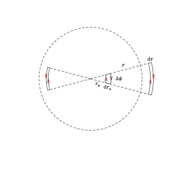
Figure 3: Images of a thin annulus from ${r_{\rm s}}$ to ${r_{\rm s}}+d{r_{\rm s}}$ by a point lens on the plane of the sky. The dashed line is the Einstein ring. $\Delta\phi$ is the angle subtended by the thin annulus. Notice that the positive image (outside the Einstein ring) is clockwise while the negative image (inside the Einstein ring) is counter-clockwise.

2.5 Light curve and microlensing degeneracy

Given a source trajectory, we can easily describe the standard light curve with a few parameters which suffers from the microlensing degeneracy.

2.5.1 Standard light curve

For convenience, we put the lens at the origin, and let the source move across the line of sight along the $x$-axis (see Fig. 4). The impact parameter in units of the Einstein radius is labeled as $u_{0}$. For convenience, we define the Einstein radius crossing time (or ‘timescale’) as

$${t_{\rm E}}=\frac{{r_{\rm E}}}{{v_{\rm t}}}=\frac{{\theta_{\rm E}}}{{\mu_{\rm rel}}},~{}~{}{\theta_{\rm E}}=\frac{{r_{\rm E}}}{{D_{\rm d}}},~{}~{}{\mu_{\rm rel}}\equiv\frac{{v_{\rm t}}}{{D_{\rm d}}},$$ (16)

where ${v_{\rm t}}$ is the transverse velocity (on the lens plane) and ${\mu_{\rm rel}}$ is the relative lens-source proper motion. Substituting the expression for the Einstein radius into Equation (11), we find that

$${t_{\rm E}}\approx 19\,\,{\rm day}\sqrt{4\times\frac{{D_{\rm d}}}{{D_{\rm s}}}\left(1-\frac{{D_{\rm d}}}{{D_{\rm s}}}\right)}\left(\frac{{D_{\rm s}}}{8\,{\rm kpc}}\right)^{1/2}\left(\frac{M}{0.3M_{\odot}}\right)^{1/2}\left(\frac{{v_{\rm t}}}{200\,{\rm km\,s^{-1}}}\right)^{-1}.$$ (17)

If the closest approach is achieved at time $t=t_{0}$, then the dimensionless coordinates are ${x_{\rm s}}=(t-t_{0})/{t_{\rm E}}$, ${y_{\rm s}}=u_{0}$ and the magnification as a function of time is given by

$$\mu(t)=\frac{{r_{\rm s}}^{2}(t)+2}{{r_{\rm s}}(t)\sqrt{{r_{\rm s}}^{2}(t)+4}},~{}~{}~{}{r_{\rm s}}(t)=\sqrt{u_{0}^{2}+\left(\frac{t-t_{0}}{{t_{\rm E}}}\right)^{2}}.$$ (18)

Two examples of light curves are shown in the right panel of Fig. 1 for $u_{0}=0.1$ and 0.3.

Figure 4: Illustration of the lens position and source trajectory. The dimensionless impact parameter is $u_{0}$, $({x_{\rm s}},{y_{\rm s}})$ is the dimensionless source position along the trajectory, and ${r_{\rm s}}$ is the distance between the lens and source.

To model an observed light curve, three parameters are present in Equation (18): $t_{0}$, ${t_{\rm E}}$, and $u_{0}$. In practice, we need two additional parameters, $m_{0}$, the baseline magnitude, and ${{\cal F}_{\rm s}}$, a blending parameter. ${{\cal F}_{\rm s}}$ characterizes the fraction of light contributed by the lensed source; in crowded stellar fields, each observed ‘star’ may be a composite of the lensed star, other unrelated stars within the seeing disk and the lens if it is luminous (Alcock et al. 2001b; Kozłowski et al. 2007). Blending will lower the observed magnification and in general ${{\cal F}_{\rm s}}$ depends on the wavelength, and so each filter requires a separate ${{\cal F}_{\rm s}}$ parameter.

Unfortunately, we can see from Equation (18) that there is only one physical parameter (${t_{\rm E}}$) in the model that relates to the lens’ properties. Since ${t_{\rm E}}$ depends on the lens mass, distances to the lens and source, and the transverse velocity ${\mu_{\rm rel}}$, from an observed light curve well fitted by the standard model, one cannot uniquely infer the lens distance and mass; this is the so-called microlensing degeneracy. However, given a lens mass function and some kinematic model of the Milky Way, we can infer the lens mass statistically.

2.6 Non-standard light curves

The standard model assumes the lensed source is point-like, both the lens and source are single and all the motions are linear. The majority ($\sim 90\%$) of microlensing events are well described by this simple model. However, about 10% of the light curves are non-standard (exotic), due to the breakdown of one (or more) of the assumptions. We briefly list these possibilities below. These non-standard microlensing events allow us to derive extra constraints, and partially lift the microlensing degeneracy. Because of this, they play a role far greater than their numbers suggest.

1. binary lens events: The lens may be in a binary or even a multiple system (Mao & Paczński 1991). The light curves for a binary or multiple lensing system can be much more diverse (see Sec. 2.7). They offer an exciting way to discover extrasolar planets (Mao & Paczński 1991; Gould & Loeb 1992; Bennett & Rhie 1996; Griest & Safizadeh 1998; Rattenbury et al. 2002, for more see Sec. 3.5).

2. binary source events: The source is in a binary system. In this case, the light curve will be a simple, linear superposition of the two sources (when the orbital motion can be neglected, see Griest & Hu 1992).

3. finite source size events: The finite size of the lensed star cannot be neglected. This occurs when the impact parameter $u_{0}$ is comparable to the stellar radius normalized to the Einstein radius, $u_{0}\sim r_{\star}/{r_{\rm E}}$. In this case, the light curve is significantly modified by the finite source size effect (Witt & Mao 1994; Gould 1994). The finite source size effect is most important for high magnification events.

4. parallax/“xallarap” events: The standard light curve assumes all the motions are linear. However, the source and/or the lens may be in a binary system, furthermore, the Earth revolves around the Sun. All these motions induce accelerations. The effect due to Earth’s motion around the Sun is usually called “parallax” (e.g. Gould 1992; Smith 2002; Poindexter et al. 2005), while that due to binary motion in the source plane is called “xallarap” (“parallax” spelt backwards, Bennett 1998; Alcock et al. 2001a). Parallax or “xallarap” events usually have long timescales. For a typical microlensing event with timescale ${t_{\rm E}}\sim 20\,{\rm day}$, the parallax effect due to the Earth rotation around the Sun is often undetectable (unless the photometric accuracy of the light curve is very high or the lens is very close).

5. Repeating events: Microlensing can “repeat”, in particular if the lens is a wide binary (Di Stefano & Mao 1996) or the source is a wide binary. In such cases, microlensing may manifest as two well-separated peaks, i.e., as a “repeating” event. A few percent of microlensing events are predicted to repeat, consistent with the observations (Skowron et al. 2009).

Notice that several violations may occur at the same time, which in some cases allow the microlensing degeneracy to be completely removed (e.g. An et al. 2002; Dong et al. 2009b; Gaudi et al. 2008).

In particular, when both finite source size and parallax effects are seen, the lens mass can be determined uniquely (Gould 1992). Microlensing parallax measures the projected Einstein radius in the observer plane (in units of the Earth-Sun separation, AU): $\tilde{r}_{\rm E}={r_{\rm E}}\times{D_{\rm s}}/{D_{\rm ds}}$, or equivalently, the parallax $\pi_{\rm E}=1\,{\rm AU}/\tilde{r}_{\rm E}$. The finite source size effect, on the other hand, measures the ratio of the angular stellar radius $\theta_{\star}$ to the angular Einstein radius ${\theta_{\rm E}}$. Since the angular size of the lensed star can be measured from its color and apparent magnitude (Yoo et al. 2004), we can derive the angular Einstein radius ${\theta_{\rm E}}$. It is straightforward to combine Eqs. (11) and (6) to obtain

$$M={c^{2}\over 4G}\tilde{r}_{\rm E}\,{\theta_{\rm E}}={c^{2}\over 4G}{{\theta_{\rm E}}\over\pi_{\rm E}}.$$ (19)

Notice that the determination is independent of all the distances.

Equation (19) is especially transparent in the natural formalism advocated by Gould (2000), which provides a way to connect quantities measurable in microlensing ($\pi_{\rm E},{\theta_{\rm E}},{t_{\rm E}}$) with other physical quantities:

$$\pi_{\rm rel}=\pi_{\rm E}{\theta_{\rm E}},~{}~{}\mu_{\rm rel}={{\theta_{\rm E}}\over{t_{\rm E}}},$$ (20)

where $\pi_{E}=1/\tilde{r}_{\rm E}$, $\pi_{\rm rel}=1/{D_{\rm d}}-1/{D_{\rm s}}$ is the lens-source relative parallax and $\mu_{\rm rel}$ is the relative proper motion (also used in equation 16). For example, if the lens and distance can be measured (using other means), then $\pi_{\rm rel}$ can be determined. In addition, if the lens and source motions can be measured, then we can determine the relative proper motions ($\mu_{\rm rel}$).

2.7 $N$-point lens gravitational microlensing

It is straightforward to derive the (dimensionless) lens equation for $N$-point lenses. We can first cast Equation (8) in vector form and then rearrange

$$\vec{{r_{\rm s}}}=\vec{{r}}-\frac{1}{|\vec{{r}}|^{2}}\vec{{r}}.$$ (21)

The above expression implicitly assumes that the lens is at the origin, and all the lengths have been normalized to the Einstein radius corresponding to its mass (or equivalently, the lens mass has been assumed to be unity).

Let us consider the general case where we have $N$-point lenses, at $\vec{r}_{k}=(x_{k},y_{k})$ with mass $M_{k}$, $k=1,\cdot\cdot\cdot,N$. We normalize all the lengths with the Einstein radius corresponding to the total mass, $M=\sum_{k=1}^{N}M_{k}$. The generalized lens equation then reads

$$\vec{{r_{\rm s}}}=\vec{{r}}-\sum_{k=1}^{N}m_{k}\frac{\vec{{r}}-\vec{r}_{k}}{|(\vec{{r}}-\vec{r}_{k})|^{2}},~{}~{}m_{k}=\frac{M_{k}}{M},$$ (22)

where $\sum_{k=1}^{N}m_{k}=1$. If there is only one lens ($m_{1}=1$) and the lens is at the origin, then Equation (22) reverts to the single lens equation (21).

Two-dimensional vectors and complex numbers are closely related, Witt (1990) first demonstrated that the above equation can be cast into a complex form by direct substitutions of the vectors by complex numbers:

$${z_{\rm s}}=z-\sum_{k=1}^{N}m_{k}\frac{z-z_{k}}{(z-z_{k})(\bar{z}-\bar{z}_{k})}=z-\sum_{k=1}^{N}\frac{m_{k}}{\bar{z}-\bar{z}_{k}},$$ (23)

where $z=x+y\,i$, $z_{k}=x_{k}+y_{k}\,i$, and ${z_{\rm s}}={x_{\rm s}}+{y_{\rm s}}\,i$ ($i$ is the imaginary unit).

We can take the conjugate of Equation (23) and obtain an expression for $\bar{z}$. Substituting this back into Equation (23), we obtain a complex polynomial of degree $N^{2}+1$. This immediately shows that 1) even a binary lens equation cannot be solved analytically since it is a fifth-order polynomial, and 2) the maximum number of images cannot exceed $N^{2}+1$. In fact, the upper limit is $5(N-1)$ (see Sec. 3.7), which indicates that most solutions of the complex polynomial are not real images of the lens equation.

The magnification is related to the determinant of the Jacobian of the mapping from the source plane to the lens plane: $({x_{\rm s}},{y_{\rm s}})\rightarrow(x,y)$. In the complex form, this is (Witt 1990):

$$\mu=\frac{1}{J},~{}~{}~{}J=\frac{\partial({x_{\rm s}},{y_{\rm s}})}{\partial(x,y)}=1-\frac{\partial{z_{\rm s}}}{\partial\bar{z}}\overline{\frac{\partial{z_{\rm s}}}{\partial\bar{z}}}.$$ (24)

Notice that the Jacobian can be equal to zero implying a (point) source will be infinitely magnified. The image positions satisfying $J=0$ form continuous critical curves, which are mapped into caustics in the source plane. Of course, stars are not point-like, they have finite sizes. The finite source size of a star smooths out the singularity. As a result, the magnification remains finite.

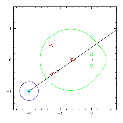
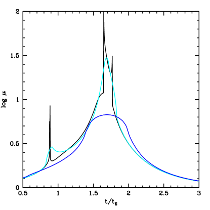
Figure 5: Left panel: Caustics (red curves) and critical curves (green curves) for a binary lens. The lenses (indicated by two ‘+’ signs) are located at $z_{1}=(-0.665,0)$ and $z_{2}=(0.035,0)$ with mass $m_{1}=0.95$ and $m_{2}=1-m_{1}=0.05$ respectively. The black line shows the trajectory for three source sizes, ${r_{\rm s}}/{r_{\rm E}}=0,0.05,0.3$, indicated by the cyan and blue circles and a dot (for a point source). The trajectory starts at $(-2,-1)$ with a slope of 0.7. Right panel: Corresponding light curves for the three source sizes along the trajectory in the left panel. The time is normalized to the Einstein radius crossing time, ${t_{\rm E}}$, and $t=0$ corresponds to the starting position. Notice that as the source size increases, the lensing magnifications around the peaks usually decrease.

For $N$-point lenses, from the complex lens equation (23), we have

$$\frac{\partial{z_{\rm s}}}{\partial\bar{z}}=\sum_{k=1}^{N}\frac{m_{k}}{(\bar{z}-\bar{z}_{k})^{2}},~{}~{}~{}J=1-\Big{|}\sum_{k=1}^{N}\frac{m_{k}}{(\bar{z}-\bar{z}_{k})^{2}}\Big{|}^{2}.$$ (25)

It follows that the critical curves are given by

$$\Big{|}\sum_{k=1}^{N}\frac{m_{k}}{(\bar{z}-\bar{z}_{k})^{2}}\Big{|}^{2}=1.$$ (26)

The sum in the above equation must be on a unit circle, and the solution can be cast in a parametric form

$$\sum_{k=1}^{N}\frac{m_{k}}{(z-z_{k})^{2}}={\rm e}^{i\Phi},$$ (27)

where $0\leq\Phi<2\pi$ is a parameter. The above equation is a complex polynomial of degree $2N$ with respect to $z$. For each $\Phi$, there are at most $2N$ distinct solutions. As we vary $\Phi$ continuously, the solutions trace out at most $2N$ continuous critical curves (critical curves of different solutions can smoothly join with each other). In practice, we can solve the equation for one $\Phi$ value, and then use the Newton-Raphson method to find the solutions for other values of $\Phi$. For a point source, the complex polynomial can be easily solved numerically (e.g. using the zroots routine in Press et al. 1992, see also Skowron & Gould 2012). However, for a source with finite size, the existence of singularities makes the integration time-consuming (see Sec. 4). The right panel in Fig. 5 shows the light curves for three source sizes along the trajectory indicated by the straight black line. As the source size increases, the lensing magnifications around the peaks usually decrease and become broader. Furthermore, the number of peaks may differ for different source sizes.

2.8 Optical depth and event rates

So far we have derived the lens equation and light curve for microlensing by a single star. In reality, hundreds of millions of stars are monitored, and $\approx 2000$ unique microlensing events are discovered each year (OGLE-IV alone identifies about 1500 microlensing events each year). Clearly we need some statistical quantities to describe microlensing experiments. For this, we need two key concepts: optical depth and event rate.

2.8.1 Optical depth

The optical depth (lensing probability) is the probability that a given source falls into the Einstein radius of any lensing star along the line of sight. Thus the optical depth can be expressed as

$$\tau=\int_{0}^{D_{\rm s}}n({D_{\rm d}})\left(\pi{r_{\rm E}}^{2}\right)d{D_{\rm d}},$$ (28)

which is an integral of the product of the number density of lenses, the lensing cross-section ($=\pi{r_{\rm E}}^{2}$) and the differential path ($d{D_{\rm d}}$).

Alternatively, the optical depth can be viewed as the fraction of sky covered by the angular areas of all the lenses, which yields another expression

$$\tau=\frac{1}{4\pi}\int_{0}^{D_{\rm s}}\left[n({D_{\rm d}})4\pi{D_{\rm d}}^{2}d{D_{\rm d}}\right]\left(\pi{\theta_{\rm E}}^{2}\right),$$ (29)

where the term in the [ ] gives the numbers of lenses in a spherical shell with radius ${D_{\rm d}}$ to ${D_{\rm d}}+d{D_{\rm d}}$, $\pi{\theta_{\rm E}}^{2}$ is the angular area covered by a single lens, and the term in the denominator is the total solid angle over all the sky ($4\pi$).

If all the lenses have the same mass $M$, then $n({D_{\rm d}})=\rho({D_{\rm d}})/M$, $\pi{r_{\rm E}}^{2}\propto M$, and the lens mass drops out in $n({D_{\rm d}})\pi{r_{\rm E}}^{2}$. Therefore the optical depth depends on the total mass density along the line of sight, but not on the mass function.

Let us consider a simple model where the density is constant along the line of sight, $\rho({D_{\rm d}})=\rho_{0}$. Integrating along the line of sight one finds

$$\tau=\frac{2\pi G\rho_{0}}{3c^{2}}{D_{\rm s}}^{2}=\frac{1}{2c^{2}}\frac{G\rho_{0}4\pi{D_{\rm s}}^{3}/3}{{D_{\rm s}}}=\frac{1}{2c^{2}}\frac{GM(<{D_{\rm s}})}{{D_{\rm s}}}=\frac{V^{2}}{2c^{2}},$$ (30)

where $M(<{D_{\rm s}})$ is the total mass enclosed within the sphere of radius ${D_{\rm s}}$ and the circular velocity is given by $V^{2}=GM(<{D_{\rm s}})/{D_{\rm s}}$.

For the Milky Way, $V\approx 220\,{\rm km\,s^{-1}}$, and $\tau\approx 2.6\times 10^{-7}$. The low optical depth means millions of stars have to be monitored to have a realistic yield of microlensing events, and thus one needs to observe dense stellar fields, which in turn means accurate crowded field photometry is essential (see Alard & Lupton 1998; Alard 2000; Wozniak 2000, 2008, and references therein).

2.9 Event rate

The optical depth indicates the probability of a given star that is within the Einstein radii of the lenses at any given instant. As such, the optical depth is a static concept. We are obviously interested in knowing the event rate (a dynamic concept), i.e., the number of (new) microlensing events per unit time for a given number of monitored stars, $N_{\star}$.

To calculate the event rate, it is easier to imagine the lenses are moving in a background of static stellar sources. For simplicity, let us assume all the lenses move with the same velocity of ${v_{\rm t}}$. The new area swept out by each lens in the time interval $dt$ is equal to the product of the diameter of the Einstein ring and the distance traveled ${v_{\rm t}}\,dt$, $dA=2{r_{\rm E}}\times{v_{\rm t}}dt=2{r_{\rm E}}^{2}dt/{t_{\rm E}}$. The probability of a source becoming a new microlensing event is given by

$$d\tau=\int_{0}^{{D_{\rm s}}}n({D_{\rm d}})dAd{D_{\rm d}}=\int_{0}^{{D_{\rm s}}}n({D_{\rm d}})\left(\frac{2{r_{\rm E}}^{2}}{{t_{\rm E}}}\right)dtd{D_{\rm d}}$$ (31)

The total number of new events is $N_{\star}d\tau$, and thus the event rate is given by

$$\Gamma=\frac{N_{\star}\,d\tau}{dt}=N_{\star}\int_{0}^{{D_{\rm s}}}n({D_{\rm d}})\left(\frac{2}{\pi{t_{\rm E}}}\cdot{\pi{r_{\rm E}}^{2}}\right)\,d{D_{\rm d}}=\frac{2N_{\star}}{\pi}\int\frac{d\tau}{{t_{\rm E}}}.$$ (32)

If, for simplicity, we assume that all the Einstein radius crossing times are identical, then we have

$$\Gamma\approx\frac{2N_{\star}}{\pi}\frac{\tau}{{t_{\rm E}}}.$$ (33)

We make several remarks about the event rate:

1. If we take ${t_{\rm E}}=19\,{\rm day}$ (roughly equal to the median of the observed timescales), then we have

   $$\Gamma\approx\frac{2N_{\star}}{\pi}\frac{\tau}{{t_{\rm E}}}=1200\,{\rm yr}^{-1}\frac{N_{\star}}{10^{8}}\frac{\tau}{10^{-6}}\left(\frac{{t_{\rm E}}}{19\,{\rm day}}\right)^{-1}.$$ (34)

   For OGLE-III, about $2\times 10^{8}$ stars are monitored, so the total number of lensing events we expect per year is $\Gamma\sim 2400$ if $\tau\sim 10^{-6}$, which is within a factor of four of the observed rate (indicating the detection efficiency may be of the order of 30%).

2. While the optical depth does not depend on the mass function, the event rate does because of ${t_{\rm E}}(\propto M^{1/2})$ in the denominator of Equation (33). The timescale distribution can thus be used to probe the kinematics and mass function of lenses in the Milky Way.

3. The lenses and sources have velocity distributions; one must account for them when realistic event rates are needed. Furthermore, the source distance is unknown, and so in general we need to average over the source distance (for example calculations, see Griest 1991; Kiraga & Paczyński 1994).

3 Applications of Gravitational Microlensing

As we can see, the theory of gravitational microlensing is relatively simple. When Paczyński (1986) first proposed microlensing, the astronomical community was very skeptical whether microlensing events could be differentiated from other types of variable stars (for an example of skepticism, see Mao 2008b). As proven again and again in the field, such pessimism is often unwarranted: with the rapid increase in the discovery rate of microlensing events (from a few events in the early years to about 2000 events annually), even small probability events can be discovered. The best example may be the seemingly crazy idea of terrestrial parallax proposed by Hardy & Walker (1995) and Holz & Wald (1996), which has subsequently been observed by Gould et al. (2009). Since the discovery of the first microlensing events in 1993, more than 10,000 events (mostly in real-time) have been discovered. In the process, tens of TBytes of data have been accumulated. This tremendous database is a treasure trove for exploring diverse astrophysical applications.

3.1 MACHOs in the Galactic halo?

Microlensing was originally proposed to detect MACHOs in the Galactic halo (Paczyński 1986). Earlier results by the MACHO collaboration suggest that a substantial fraction ($\approx 20\%$) of the halo may be in MACHOs (Alcock et al. 2000) based on 13-17 events toward the Large Magellanic Cloud (LMC) in 5.7 years of data. The number of events quoted here varies somewhat depending on the selection criteria, which is a debated point (see, e.g., Belokurov et al. 2004; Bennett 2005; Griest & Thomas 2005; Evans & Belokurov 2007).

In any case, the result turns out to be controversial, as these numbers are not confirmed by the EROS (Tisserand et al. 2007) or OGLE collaborations (Wyrzykowski et al. 2011). A recent analysis of the OGLE data toward the LMC concluded only $\la 2\%$ of the halo could be in MACHOs (Wyrzykowski et al. 2011) - all events can be explained by lensing by normal stars. In fact, at least two of the MACHO events turn out to be by stars in the thick disk of the Milky Way (Drake et al. 2004; Kallivayalil et al. 2006). The lack of MACHOs is entirely consistent with the baryonic content determined from many other astrophysical observations (e.g. from microwave background observations, Komatsu et al. 2011).

3.2 Galactic Structure

Microlensing data offer a number of ways to study the Galactic structure, which is still somewhat under-explored, and more work is needed.

3.2.1 Color-Magnitude Diagrams

Microlensing surveys yield many high-quality color-magnitude diagrams of stellar populations over hundreds of square degrees. Such data contain much information about stellar populations in the bulge. Despite of some promising earlier attempts (e.g. Ng et al. 1996), not much work has been done since due to the difficulty of disentangling the dust extinction, spatial distributions and complexities in the stellar populations (see the next subsections). It is nevertheless worthwhile to perform further analyses in this area.

3.2.2 Red Clump Giants As Standard Candles

Red clump giants are metal-rich, core-helium burning horizontal branch stars. They have approximately constant luminosity (standard candles) (Paczyński & Stanek 1998) and relatively little dependence on the metallicities, especially in the $I$-band (see Udalski 1998a; Zhao et al. 2001; Nataf & Udalski 2011, and references therein). As such, they can be used to determine the distances to the Galactic center and the Magellanic Clouds (Udalski 1998b). This complements the determination of other standard candles such as RR Lyrae stars and Cepheids (Groenewegen et al. 2008). The distance to the Galactic center determined with these methods is typically very close to 8 kpc, with a combined systematic and statistical error of about 5%.

The observed width of red clump giants in a given line-of-sight toward the Galactic center is larger than their intrinsic scatters ($\approx 0.2$ mag) because of the finite depth of the Galactic bar. A careful analysis of the counts of red clump giants can be used to determine the geometric parameters of the bar. For example, for 44 fields from the OGLE-II data, the three axial lengths are found to be close to 10:3.5:2.6 with a bar angle of 24-27^∘ (Rattenbury et al. 2007a), largely consistent with the earlier study by Stanek et al. (1997). Extra care, however, needs to be taken for fields off the plane due to the presence of two red clump populations (Nataf et al. 2010), which suggests an X-shaped structure in the Milky Way center (see also McWilliam & Zoccali 2010; Saito et al. 2011).

We note that the OGLE-III and OGLE-IV campaigns cover much larger areas on the sky, which can be used to constrain not only the bar but perhaps also spiral arm structures. Investigations taking this approach are already under way (Nataf et al. 2012, in preparation).

3.2.3 Extinction Maps

Red clump giants can also be used to infer extinctions toward the Galactic Center. The first application of this method to the OGLE-I data was performed by Stanek (1996) and later to the OGLE-II data by Sumi (2004). The extinction maps are approximately consistent with those obtained with other methods (e.g. Schlegel et al. 1998). One interesting conclusion from these studies is that the extinction law is almost always anomalous toward the Galactic center (Udalski 2003).

A very recent application of the method to the VISTA Variables in the Via Lactea (VVV) survey can be found in Gonzalez et al. (2012).

3.2.4 Proper Motions

Nearly two decades of time series of observations for many different bulge fields offer a way to determine stellar proper motions. This has been done for the OGLE-II catalog for about five million stars with an accuracy of $\sim{\rm mas\,yr^{-1}}$ (see Sumi et al. 2004 and Rattenbury & Mao 2008 for a study of selected high-proper motion stars).

One particularly interesting issue concerns the anisotropy in the bulge kinematics. The proper motion dispersions in the longitudinal and latitudinal directions have ratios close to $\approx 0.9$; these values are similar to those independently measured with the Hubble Space Telescope in a number of fields but for a smaller number of stars (Kozłowski et al. 2006; Clarkson et al. 2008). A comparison with theoretical predictions seems to indicate that the theoretical models are too anisotropic (Rattenbury et al. 2007b).This effect is also seen in more recent modelling with the Schwarzschild method (Wang et al. 2012). The reason for this discrepancy is not completely clear. One issue worth mentioning is that bulge observations are often contaminated by disk stars, a point emphasized by Vieira et al. (2007).

3.2.5 Optical Depths and Galactic bar

In Sec. 2.8, we showed that the optical depth provides an independent probe of the density distribution in the bulge. Earlier determinations of the optical depth in the Baade Window have provided independent evidence that the Galactic bulge contains a bar (Kiraga & Paczyński 1994; Zhao et al. 1996). While we have discovered about ten thousand microlensing events over the last two decades, only a small fraction has been used for statistical analyses of optical depths.

More recent determinations of microlensing optical depths have been performed by Hamadache et al. (2006) using 120 red clump giants from the EROS collaboration, 60 red clump giants from the MACHO collaboration (Popowski et al. 2005), 28 events for the MOA collaboration (Sumi et al. 2003) and 32 high signal-to-noise ratio events for the OGLE collaboration (Sumi et al. 2006). The measured optical depths are largely consistent with theoretical predictions (e.g., Wood & Mao 2005; Ryu et al. 2008; Kerins et al. 2009).

The reason that the measurements have only been performed for red clump giants is that they are bright and are supposed to suffer less from the blending in the crowded bulge field (in fact, this is not rigorously true, see Sumi et al. 2006). If we can overcome this and the issue of human resources (see the next subsection), combined with the number counts of red clump giants, we can in principle constrain the bulge density distribution much better using non-parametric models. For example, we can use non-parametric models rather than the simple parametric models often used in the literature (still based on very poor-resolution [$\approx 7^{\circ}$] maps from DIRBE on COBE, Dwek et al. 1995).

3.2.6 Timescale Distributions and Mass Functions

As we have seen in Sec. 2.9, the timescale distribution of event rates carries information about the mass function of lenses. An early study by Han & Gould (1995) of 51 events concluded that for a power-law mass function, $n(M)dM\sim M^{-\beta}\,dM$, the preferred slope $\beta\approx 2.1$, with a lower mass cutoff of about $0.04M_{\odot}$. Their slope is close to the Salpeter value ($\beta=2.35$). The study by Zhao et al. (1996) also concluded that the data are inconsistent with a large population of brown dwarfs in the bulge. A more recent analysis by Calchi Novati et al. (2008) modeled the mass function and found $\beta\approx 1.7\pm 0.5$. The large error bar is again due to the small number of events used ($\sim 100$).

The current data base contains roughly two orders of magnitude more events - it would be very interesting to explore what we can learn with the full data set we now possess. However, there are at least two difficulties that will need to overcome. One is human resources: extensive Monte Carlo simulations must be performed to determine the completeness of surveys - this will be a time-consuming exercise. Secondly, the effect of blending of background stars needs to be taken into account (see Sec. 2.5.1). This is not so straightforward since the fields have different degrees of crowding (Smith et al. 2007). Nevertheless, it will be valuable to perform an analysis of the optical depth maps and timescale distributions using all the data set to understand the density map and mass functions of the bulge and mass of the disk. Notice that the microlensing sample is largely a mass-selected sample, rather than a light-selected sample as in most other studies.

This exercise may be particularly interesting in light of evidence for systematic variations in the initial mass functions in elliptical galaxies from both dynamics (Cappellari et al. 2012) and strong gravitational lensing (Treu et al. 2010). A careful study of the mass functions in the bulge and disk from microlensing offers an important independent check on these conclusions by investigating whether the Galactic bulge follows similar trends.

3.3 Stellar atmosphere and bulge formation

High-magnification events offer great targets-of-opportunity to obtain spectra with high signal-to-noise ratio to study stellar atmospheres in bulge stars (Lennon et al. 1996). More recent observations using 8m class telescopes allow determinations of a number of stellar parameters such as surface gravity, metallicity and ages (e.g. Lennon et al. 1996; Thurl et al. 2006; Cohen et al. 2008).

The most recent studies by Bensby et al. (2010, 2011) of 38 stars indicate that for dwarf stars, there may be two populations of stars. The metal-poor population seems to be predominantly old (age $\sim$ 12 Gyr) while the metal-rich population appears to have a bi-modal distribution: one is old ($\sim$ 12 Gyr) while the other one is intermediate age (3-4 Gyr). The existence of intermediate age stars seems to be in conflict with broad-band color and spectroscopy of giants (e.g. Zoccali et al. 2008). One way to resolve this conflict is that the age estimate may be incorrect due to enhanced helium enrichment (Nataf et al. 2011). While more microlensed stars are desirable, it demonstrates the power of microlensing as a natural telescope, similar to clusters of galaxies as a natural telescope to study very high-redshift galaxies.

The surface brightness of a star is not uniform, instead its limb usually appears darker (“limb-darkening”). Limb-darkening profiles have been measured for the Sun and a few other stars. The sharp magnification gradient in high-magnification or caustic-crossing events allows us to study the limb-darkening profile as the source moves across the line of sight or caustics. Notice that limb-darkening profiles can not only be studied in broad-band but also in spectral lines such as H$\alpha$ if one has time-resolved spectra during microlensing (Thurl et al. 2006).

Approximately 10 G and K giants had their limb-darkening profiles measured with microlensing (Cassan et al. 2006; Thurl et al. 2006; Zub et al. 2011). These studies suggest that “the classical laws are too restrictive to fit well the microlensing observations” (Cassan et al. 2006), and radiative transfer models will need to be improved.

3.4 Mass Determinations of Isolated Stars: from Brown Dwarfs to Stellar Mass Black Holes

As shown in Sec. 2.5.1, for standard microlensing events, the lens mass cannot be determined uniquely. However, for exotic events, partial or complete removal of this degeneracy is possible (see equation 19). Microlensing thus provides an important new way to determine the mass of isolated stars.

All stellar black hole candidates in the Milky Way are in binary systems and have been discovered through X-ray emissions (see Remillard & McClintock 2006 for a review). Their masses range from $5M_{\odot}$ to $30M_{\odot}$. Microlensing provides an independent way to study isolated black holes. The principle is very simple: Typical microlenses have masses of about $0.3M_{\odot}$, black holes are $\ga 10$ more massive, and so events due to stellar mass black holes should be a factor of a few longer. These events thus have a much larger chance of exhibiting parallax signatures, which can be used to determine the lens as a function of distance. Combined with a mass density and kinematic models of the Milky Way, we can constrain the lens mass. If it is higher than a few solar masses and it is dark (as can be inferred from the light curve from the blending parameter ${{\cal F}_{\rm s}}$, see Sec. 2.5.1), then it is a potential stellar mass black hole candidate.

Half a dozen or so such candidates have been identified by (Mao et al. 2002; Bennett et al. 2002, see also Agol et al. 2002; Poindexter et al. 2005). A search for the X-ray emission in one of the candidates, MACHO-96-BLG-5, yielded only an upper limit (Maeda et al. 2005; Nucita et al. 2006), consistent with the system being a truly isolated black hole.

An ambitious 3-year HST survey (192 orbits) is under way by a team led by K. Sahu to detect microlensing events caused by non-luminous isolated black holes and other stellar remnants. It will be very interesting to see the results from this survey (Sahu et al. 2012).

Other direct mass measurements have also been performed, especially for highly magnified microlensing events. The determined masses range from brown dwarf candidates (Smith et al. 2003b; Gould et al. 2009; Hwang et al. 2010) to more normal stars (see, e.g., Batista et al. 2009 and references therein).

3.5 Extrasolar Planets

Undoubtedly the highlight of gravitational microlensing in the last decade has been the discovery of extrasolar planets. At the time of writing, about 20 microlensing extrasolar planets have been discovered, including 16 published (Bond et al. 2004; Udalsk et al. 2005; Beaulieu et al. 2006; Gould et al. 2006; Bennett et al. 2008; Gaudi et al. 2008; Dong et al. 2009b; Janczak et al. 2010; Sumi et al. 2010; Miyake et al. 2011; Batista et al. 2011; Muraki et al. 2011; Yee et al. 2012; Bachelet et al. 2012; Bennett et al. 2012). Of these, 11 are high-magnification events, demonstrating they are excellent candidates for hunting planets, as pointed out by (Griest & Safizadeh 1998; Rattenbury et al. 2002). While this is a small fraction of the 800 extrasolar planets discovered so far, they occupy a distinct part of the parameter space which would be difficult to access with other methods (see below).

The method itself was proposed more than 20 years ago (Mao & Paczński 1991; Gould & Loeb 1992). In the abstract of Mao & Paczński (1991), it was optimistically claimed that “A massive search for microlensing of the Galactic bulge stars may lead to a discovery of the first extrasolar planetary systems.” Paczyński, however, mentioned the idea as “science fiction” at the 1991 Hamburg gravitational lensing conference. In reality, it took more than a decade of microlensing observations for the first convincing extrasolar planet to be found (Bond et al. 2004), with heroic efforts in between. Much of the theory and observations have been reviewed by Rattenbury (2006) and Gaudi (2010); we refer the readers to those papers for further details.

Fig. 6 shows an example of an extrasolar planet discovered by microlensing. The extrasolar planet has a mass of around $5.5M_{\earth}$, manifested as a secondary bump on the declining wing of the light curve, lasting for about one day. This illustrates that to find an extrasolar planet, the dense sampling of light curves plays a critical role.

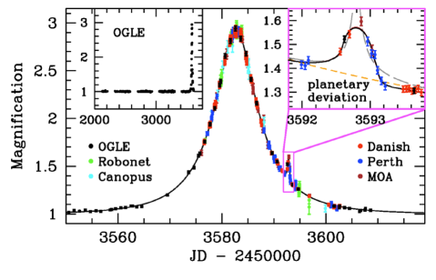
Figure 6: A super-Earth ($\approx 5.5M_{\earth}$) discovered by microlensing. Different symbols indicate data from different observatories; the solid line shows the best-fit model(s). The two insets show the OGLE data alone and the planetary bump lasting for about a day. Reprinted by permission from Macmillan Publishers Ltd: Nature 439: 437-440, ©2006.

The first two-planet system discovered by Gaudi et al. (2008) through monitoring of high magnification events is shown in Fig. 7. The light curve in this case is much more dramatic due to the complex caustics involved (the top left inset) and orbital motion in the system (see Penny et al. 2011 for detailed predictions). The mass and separations of the two planets are very much like those for the Saturn and Jupiter in our solar system. Such multiple planet systems constitute about 10% of the extrasolar planets discovered through microlensing. Many multiple planetary systems have been discovered in radial velocity and transit surveys (e.g., Wright et al. 2009; Fabrycky et al. 2012 and references therein). In radial velocity surveys, at least 28% of known planetary systems appear to contain multiple planets (Wright et al. 2009). However, these two fractions cannot be easily compared since the planets discovered are at very different separations from the host stars. Furthermore microlensing is only sensitive to planets within a narrow range of the Einstein radius. A more detailed comparison is needed to address this issue.

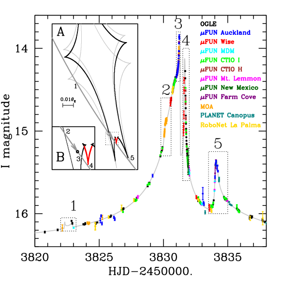
Figure 7: The first two-planet system discovered by Gaudi et al. (2008). Different symbols are data taken from different telescopes (12 in total). The numbers indicate different features produced by caustic crossings and orbital motions. From Science, Volume 319, no. 5865, pp. 927-930. Reprinted with permission from AAAS.

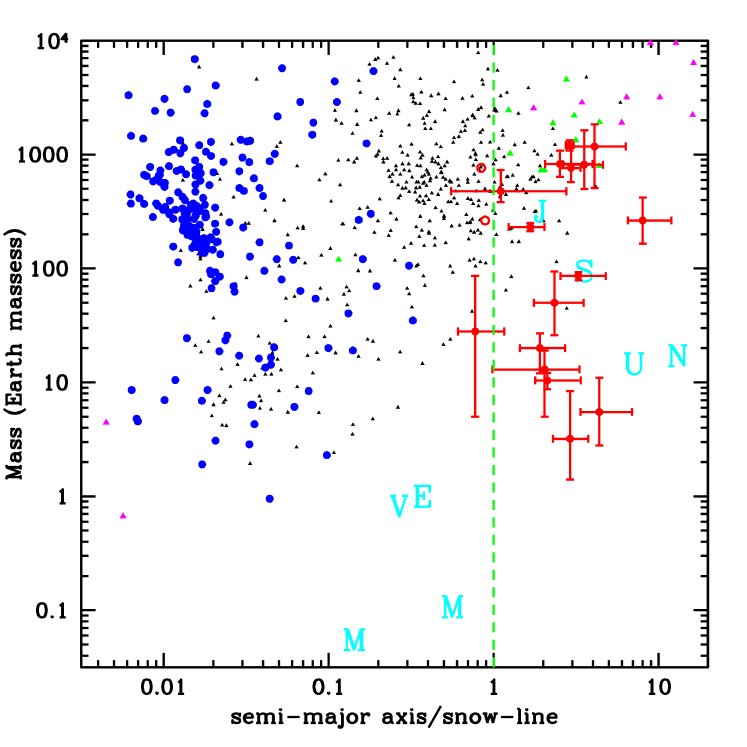
Figure 8: Extrasolar planets in the plane of mass vs. separation (in units of the snow line, indicated by the vertical dashed green line). The snow line is taken to be at $\approx 2.7M_{\rm L}/M_{\odot}$  AU, where $M_{\rm L}$ is the lens mass (see Table 1). The red filled circles with error bars indicate planets found by microlensing. The open symbols show the degenerate close-separation solutions for MOA-2007-BLG-400Lb and MOA-2011-BLG-293Lb (see Table 1). The black triangles and blue squares indicate the planets discovered by radial velocities and transits, respectively. The magenta and green triangles indicate the planets detected via direct imaging and timing, respectively. The non-microlensing exoplanet data were taken from The Extrasolar Planets Encyclopaedia (http://exoplanet.eu/). The planets in our solar system are indicated with initial letters (in cyan).

Table 1 lists all the published extrasolar planets discovered by microlensing at the time of writing. This is an expanded version of Table 3 in Miyake et al. (2011). The microlensing planets occupy a distinct part in the plane of mass vs. separation normalized by the snow line. This is illustrated in Fig. 8. It is seen that microlensing planets reside mostly outside the snow line where their equilibrium temperatures are low, about 100 K (see also, e.g., Fig. 3 in Beaulieu et al. 2008). Beyond the snow line, the density of solid particles in the disk increases rather abruptly, the planetesimal cores can form faster and the formation of gas giants becomes easier. The equilibrium temperatures are very different from the hot planets found, for example, in radial velocity searches.

Analyses of microlensing extrasolar planets has already yielded very interesting statistical results on planet frequency. Surprisingly, six high-magnification events appear to form a well-defined “sample” (Gould et al. 2010) even though the observations by the followup teams were triggered by somewhat chaotic human involvement. The authors presented the first measurement of the planet frequency beyond the snow line, for the planet-to-star mass-ratio interval $-4.5<\log q<-2$, corresponding to the range of ice giants to gas giants. The frequency was found to follow ${d^{2}N_{\rm pl}/d\log q/d\log s}=(0.36\pm 0.15){\rm dex}^{-2}$, where $q$ is the mass ratio and $s$ is the separation. This is consistent with the extrapolation of Cumming et al. (2008) to large separations. Their study also implies a first estimate of 1/6 for the frequency of solar-like systems.

More recently, Cassan et al. (2012) reported a statistical analysis of microlensing data (gathered in 2002-07) and concluded that about 20% stars host Jupiter-mass planets (between 0.3 and 10  Jupiter masses) while cool Neptunes ($10-30 M_{\earth}$) and super-Earths ($5-10 M_{\earth}$) are even more common: their abundances per star are close to 60%.

Table 1: Parameters of exoplanets discovered by microlensing.

Name	Host Star Mass	Distance	Planet Mass	Separation	Mass estimated by	References
	$M_{\rm L}(M_{\odot})$	$D_{\rm L}$(kpc)	$M_{\rm p}$	$a$(AU)
OGLE-2003-BLG-235Lb	$0.63^{\ +0.07}_{\ -0.09}$	$5.8^{\ +0.6}_{\ -0.7}$	$2.6^{\ +0.8}_{\ -0.6}\ M_{\rm J}$	$4.3^{\ +2.5}_{\ -0.8}$	$\theta_{\rm E}$, LB	1, 2
OGLE-2005-BLG-071Lb	$0.46\pm 0.04$	$3.2\pm 0.4$	$3.8\pm 0.4\ M_{\rm J}$	$3.6\pm 0.2$	$\theta_{\rm E},\pi_{\rm E}$, DL	3, 4
OGLE-2005-BLG-169Lb	$0.49^{\ +0.23}_{\ -0.29}$	$2.7^{\ +1.6}_{\ -1.3}$	$13^{\ +6}_{\ -8}\ M_{\oplus}$	$2.7^{\ +1.7}_{\ -1.4}$	$\theta_{\rm E}$, Bayesian	5
OGLE-2005-BLG-390Lb	$0.22^{\ +0.21}_{\ -0.11}$	$6.6^{\ +1.0}_{\ -1.0}$	$5.5^{\ +5.5}_{\ -2.7}\ M_{\oplus}$	$2.6^{\ +1.5}_{\ -0.6}$	$\theta_{\rm E}$, Bayesian	6
OGLE-2006-BLG-109Lb	$0.51^{\ +0.05}_{\ -0.04}$	$1.49\pm 0.19$	$231\pm 19\ M_{\oplus}$	$2.3\pm 0.5$	$\theta_{\rm E},\pi_{\rm E}$	7
c			$86\pm 7\ M_{\oplus}$	$4.5^{\ +2.1}_{\ -1.0}$	$\theta_{\rm E},\pi_{\rm E}$	7
OGLE-2007-BLG-368Lb	$0.64^{\ +0.21}_{\ -0.26}$	$5.9^{\ +0.9}_{\ -1.4}$	$20^{\ +7}_{\ -8}\ M_{\oplus}$	$3.3^{\ +1.4}_{\ -0.8}$	$\theta_{\rm E}$, Bayesian	8
MOA-2007-BLG-192Lb	$0.084^{\ +0.015}_{\ -0.012}$	$0.70^{\ +0.21}_{\ -0.12}$	$3.2^{\ +5.2}_{\ -1.8}\ M_{\oplus}$	$0.66^{\ +0.19}_{\ -0.14}$	$\theta_{\rm E},\pi_{\rm E}$	9
MOA-2007-BLG-400Lb	$0.30^{\ +0.19}_{\ -0.12}$	$5.8^{\ +0.6}_{\ -0.8}$	$0.83^{\ +0.49}_{\ -0.31}\ M_{\rm J}$	$0.72^{\ +0.38}_{\ -0.16}\ /\ 6.5^{\ +3.2}_{\ -1.2}$	$\theta_{\rm E}$, Bayesian	10a
MOA-2008-BLG-310Lb	$0.67\pm 0.14$	$>6.0$	$28^{\ +58}_{\ -23}\ M_{\oplus}$	$1.4^{\ +0.7}_{\ -0.3}$	$\theta_{\rm E}$, Bayesian	11b
MOA-2009-BLG-319Lb	$0.38^{\ +0.34}_{\ -0.18}$	$6.1^{\ +1.1}_{\ -1.2}$	$50^{\ +44}_{\ -24}\ M_{\oplus}$	$2.4^{\ +1.2}_{\ -0.6}$	$\theta_{\rm E}$, Bayesian	12
MOA-2009-BLG-387Lb	$0.19^{\ +0.30}_{\ -0.12}$	$5.7^{\ +2.2}_{\ -2.2}$	$2.6^{\ +4.2}_{\ -1.6}\ M_{\rm J}$	$1.8^{\ +0.9}_{\ -0.7}$	$\theta_{\rm E}$, Bayesian	13
MOA-2009-BLG-266Lb	$0.56\pm 0.09$	$3.04{\pm 0.33}$	$10.4{\pm 1.7}M_{\oplus}$	$3.2^{\ +1.9}_{\ -0.5}$	$\theta_{\rm E}$, $\pi_{\rm E}$	14c
MOA-2011-BLG-293Lb	$0.44^{\ +0.27}_{\ -0.17}$	$7.15\pm 0.65$	$2.4^{\ +1.2}_{\ -0.6}M_{\rm J}$	$1.0\pm 0.1$/$3.5\pm 0.5$	$\theta_{\rm E}$, Bayesian	15d
MOA-2010-BLG-477Lb	$0.67^{\ +0.33}_{\ -0.13}$	$2.3\pm 0.6$	$1.5^{\ +0.8}_{\ -0.3}M_{\rm J}$	$2^{+3}_{-1}$	$\theta_{\rm E}$, Bayesian	16d
MOA-bin-1	$0.75^{\ +0.33}_{\ -0.41}$	$5.1^{+1.2}_{1.9}$	$3.7\pm 2.1M_{\rm J}$	$8.3^{+4.5}_{-2.7}$	$\theta_{\rm E}$, Bayesian	17

a MOA-2007-BLG-400Lb has two solutions due to a strong close/wide model degeneracy (see Sec. 3.7). bDetails of the MOA-2008-BLG-310Lb parameters are discussed by Janczak et al. (2010) and Sumi et al. (2010). The error bars take into account the degeneracy. c90% confidence limit. dThe system has two solutions due to a close/wide separation degeneracy (see Sec. 3.7), thus two separations are given from a Bayesian analysis assuming the lens is a main sequence star. The close separation is slightly favored. LB: lens brightness; DL: detection of the lens. 1. Bond et al. (2004); 2. Bennett et al. (2006); 3. Udalsk et al. (2005); 4. Dong et al. (2009a); 5. Gould et al. (2006); 6. Beaulieu et al. (2006); 7. Gaudi et al. (2008); 8. Sumi et al. (2010); 9. Bennett et al. (2008); 10. Dong et al. (2009b); 11. Janczak et al. (2010); 12. Miyake et al. (2011); 13. Batista et al. (2011); 14. Muraki et al. (2011); 15. Yee et al. (2012); 16. Bachelet et al. (2012); 17. Bennett et al. (2012).

Somewhat controversially, the study by Sumi et al. (2011) found a population of free-floating Jupiters, with 1.8 Jupiters per star on average. These planets are not bound to any parent stars, observationally they manifest as very short-time scale events (in contrast to very long events for stellar mass black hole candidates). Whether such a high frequency of free-floating Jupiter-mass planets can be produced in core accretion theory or gravitational instability theory is unclear.

3.6 Numerical Methods in Modelling Binary and Multiple Light Curves

The modeling of light curves can be naturally divided into two parts: The efficient calculation of light curves and finding the best-fit models in a $\chi^{2}$ sense. We refer the readers to Bennett (2010) for an excellent discussion of this topic.

3.6.1 Calculation of light curves

For a single lens, the image magnifications and positions are analytical. The light curve calculation is straightforward, even accounting for finite source size (Witt & Mao 1994).

For a finite size source lensed by a binary or multiple system, its magnification can be calculated in three different regimes with increasing complexities.

• When the source is far away from the caustics or any sharp magnification gradient, then the point source approximation can be used. In this case, the magnification can be readily found by solving the fifth-order or the tenth-order polynomials for binary or triple lens systems (e.g. using the zroots routine in Press et al. 1992; for a more efficient implementation avaliable publically see Skowron & Gould 2012). In practice, as the source moves along its trajectory, we can feed the image positions from the previous step as the initial guesses and use the Newton-Raphson (Simpson 1740) method to achieve rapid convergence to new solutions for the current source position. These can be used to deflate the polynomial to a lower-order one, which can then be solved much more easily.

  In the case of binary lensing, the deflated polynomial is usually either linear or quadratic and its solutions can then be found analytically. In this approach, we, at all times, keep all the five solutions to the polynomial (not all are true solutions of the lens equation). This efficient method was used in the first attempt to predict binary light curves Jaroszyński & Mao (2001); it is similar to Skowron & Gould (2012) in spirit. We note that for five-image configurations, the total magnification of positive-parity images must exceed that of negative-parity images by unity (Witt & Mao 1995). This can be used as a test of numerical accuracy.

• When the source is moderately (one diameter or so) far away from the caustics, the magnification can be efficiently calculated using the hexadecapole approximation proposed by Gould (2008). It has the advantage of being very efficient and at the same time providing an estimate of the approximate accuracy (see also Pejcha & Heyrovský 2009).

• When the source is approximately within one diameter of the caustics, the magnification for a finite source size calculation becomes complex and time-consuming due to the presence of singularities. Many methods have been proposed, including (modified) rayshooting (Rattenbury et al. 2002; Dong et al. 2006), level contouring (based on Stokes theorem, Gould & Gaucherel 1997; Dominik 2007) and grid integration (Bennett & Rhie 1996; Bennett 2010). For detailed comparisons between these methods, see Bennett (2010). It is clear that there is still room for improvement. Furthermore, several independent modeling codes are desirable for cross-checks.

3.6.2 Finding the global minimum

Once a binary or multiple light curve can be efficiently calculated, it still remains a highly non-trivial job to find the best-fit parameters, especially in the presence of degeneracy (see Sec. 3.7). Starting from an initial guess of the parameters, many routines can be used to converge to a local minimum using, e.g., MINUIT or GSL routines . More recently the Monte Carlo Markov Chain method has gained popularity (e.g. Dong et al. 2006; Bennett 2010).

However, to find the global minimum, often a grid of initial guesses are used. This may be, however, impractical once the dimension of the parameter space increases, especially for multiple lenses (for a nice discussion of the parameters in binary lensing including parallax and orbital motion, see Skowron et al. 2011). This may be particularly severe when the next-generation experiments come online; this area deserves much more research in the future (see Bennett 2010 for the current state of affairs).

3.7 Mathematics of Gravitational Microlensing

Gravitational lensing is mathematically rich and is related to singularity (catastrophe) theory (see the monograph by Petters et al. 2001).

In classical Keplerian potential theory, the two-body problem is analytically tractable. In gravitational lensing, as we have shown in Sec. 2.7, it is not even possible to solve the binary lens equation analytically. Curiously, for binary lenses, there is still an analytical theorem that five-image configurations must have a magnification no smaller than 3 (Witt & Mao 1995; Rhie 1997). This was used to infer the presence of blending in gravitational microlensing (Witt & Mao 1995).

In binary lensing, there is a degeneracy found by Dominik (1999) between close and wide separation binaries. This was later explored in much greater detail by An (2005). Planetary and binary lens light curves can also mimic each other (Choi et al. 2012). It is unclear whether some of these degeneracies can be generalized to multiple ($N\geq 3$) lenses. For parallax events, there are also degeneracies (Smith et al. 2003a; Gould 1995).

The number of critical curves for $N$-point lenses cannot exceed $2N$ (see Sec. 2.7). The upper bound on the number of images for $N$-point lenses is $5(N-1)$ (Rhie 2003; Khavinson & Neumann 2006). It is unclear whether these two linear scalings are related in a topological sense (see Rhie 2001, 2003; An & Evans 2006).

4 Future of Gravitational Microlensing

The future of gravitational microlensing is bright. In terms of current experiments, OGLE-IV already has a field of view of 1.4 square degrees and is readily identifying about 1500 events in real-time per year. The rate can in principle be increased by $\sim 40\%$ by analyzing their archives.

The 1.8m MOA-II telescope has a field of view of 2.2 square degrees and the MOA collaboration issues about 600 microlensing alerts each year. The MOA collaboration uses difference image analysis photometry to issue alerts, which can identify faint source stars that are undetectable when unmagnified. This is in contrast to the OGLE, which to date has only been triggered by stars identified using their template image. The MOA strategy appears to increase the alert rate by roughly a factor of $\sim 1.4$ compared to OGLE.

There has also been an influx of new telescopes involved in microlensing, including the WISE Observatory which is conducting an independent survey. In the future, more telescopes may engage in microlensing campaigns, including the SKYMAPPER. Also, Chinese astronomers are discussing possible monitoring from Antarctica (Dome-A) and Argentina where 2m class telescopes have been proposed by the Chinese Academy of Sciences. The superior seeing and continuous time coverage for a few months per year at Dome-A may be an advantage for microlensing (although the seeing is degraded due to the high air mass, Wang et al. 2009). In fact, as the first step, the first of three 50 cm telescopes has already been installed at Dome-A in early 2012 and will perform pilot surveys.

In terms of hunting for extrasolar planets, several White Papers (Gould et al. 2007; Bennett et al. 2007; Dominik 2008; Beaulieu et al. 2008) set out strategies with ambitious milestones for the next fifteen years.

• Current extrasolar discovery with microlensing is a mixture of surveys and intense followup observations. However, the boundary between surveys and followup teams is already starting to blur, with survey teams for some fraction of their time, engaging in very dense monitorings of some fields, for example, by both the MOA (Sumi et al. 2011) and OGLE teams.

• In the next five years, a network of three 1.6m telescopes will be built by Korean astronomers (Korean Microlensing Network, KMTNet). These telescopes will be sited in Chile, South Africa and Australia. Each is equipped with a 4 square degree field camera, and will be able to monitor 16 square degrees and densely sample light curves (every 10 minutes or so). This will in principle get rid of the cumbersome division between survey and followup. As a result, the selection functions will be much better specified and thus statistical studies will be easier to perform. This is important as the number of microlensing extrasolar planets will increase significantly.

• A microlensing telescope in space in the next 10-15 years has been proposed both in the US and Europe. WFIRST is the top recommended space mission by the US Decadal Survey (Blandford et al. 2010). The recently funded Euclid mission by ESA may also have a microlensing component (for detailed simulations, see Penny et al. 2012). Observing from space has substantial advantages: smaller and more stable PSFs and continuous time coverage will allow us to search for lower-mass (Earth-mass) planets. Space missions will also allow us to uniquely determine the masses of many extrasolar planets. Combined with the stellar transit mission Kepler, space microlensing experiment(s) will provide a complete census of Earth-mass (and lower-mass) planets at virtually all separations, including free-floating ones.

The theory of microlensing is well understood, although computationally there are still some challenging issues (see Sec. 3.6). For example, it is still time-consuming to calculate the light curves for finite-size sources since we need to integrate over the singularities of caustics. This is particularly important for the discovery of extrasolar planets when a source transits the small caustics induced by the planet(s). The problem becomes even worse for multiple planets (Gaudi et al. 2008). How do we efficiently search the high dimensional parameter space? Are there hidden multiple planetary light curves in the database that are not yet identified due to their complex shapes?

With a very healthy interplay between theory and observations, upgraded/new surveys in the near term and space satellites on the horizon, microlensing can expect another exciting decade in the future.