OGLE-2017-BLG-0173Lb: Low Mass-Ratio Planet in a “Hollywood” Microlensing Event

Abstract

We present microlensing planet OGLE-2017-BLG-0173Lb, with planet-host mass ratio either $q\simeq 2.5\times 10^{-5}$ or $q\simeq 6.5\times 10^{-5}$, the lowest or among the lowest ever detected. The planetary perturbation is strongly detected, $\Delta\chi^{2}\sim 10,000$, because it arises from a bright (therefore, large) source passing over and enveloping the planetary caustic: a so-called “Hollywood” event. The factor $\sim 2.5$ offset in $q$ arises because of a previously unrecognized discrete degeneracy between Hollywood events in which the caustic is fully enveloped and those in which only one flank is enveloped, which we dub “Cannae” and “von Schlieffen”, respectively. This degeneracy is “accidental” in that it arises from gaps in the data. Nevertheless, the fact that it appears in a $\Delta\chi^{2}=10,000$ planetary anomaly is striking. We present a simple formalism to estimate the sensitivity of other Hollywood events to planets and show that they can lead to detections close to, but perhaps not quite reaching, the Earth/Sun mass ratio of $3\times 10^{-6}$. This formalism also enables an analytic understanding of the factor $\sim 2.5$ offset in $q$ between the Cannae and von Schlieffen solutions. The Bayesian estimates for the host-mass, system distance, and planet-host projected separation are $M=0.39^{+0.40}_{-0.24}\,M_{\odot}$, $D_{L}=4.8^{+1.5}_{-1.8}\,{\rm kpc}$, and $a_{\perp}=3.8\pm 1.6\,{\rm AU}$. The two estimates of the planet mass are $m_{p}=3.3^{+3.8}_{-2.1}\,M_{\oplus}$ and $m_{p}=8^{+11}_{-6}\,M_{\oplus}$. The measured lens-source relative proper motion $\mu=6\,{\rm mas}\,{\rm yr}^{-1}$ will permit imaging of the lens in about 15 years or at first light on adaptive-optics imagers on next-generation telescopes. These will allow to measure the host mass but probably cannot resolve the planet-host mass-ratio degeneracy.

1 Introduction

Planetary companions of microlensing hosts induce two classes of caustic structures on the otherwise smooth magnification pattern due to the host itself; “central caustics” that lie projected close to the host and “planetary caustics” that are separated from the host position by $(s-s^{-1})\theta_{\rm E}$, where $s\theta_{\rm E}$ is the planet-star angular separation and $\theta_{\rm E}$ is the angular Einstein radius (Mao & Paczyński, 1991; Gould & Loeb, 1992; Gaudi, 2012).

For planets that lie outside the Einstein ring $(s>1)$, each of the two caustics may be regarded as due to the tidal shear induced by the other body on its own symmetric gravitational field, a regime that was first analyzed in a cosmological context by Chang & Refsdal (1984), and then in a microlens-planet context by Gould & Loeb (1992). Since the Einstein radius $\theta_{\rm E}$ of each is proportional to the square root of the lens mass $M$,

$$\theta_{\rm E}\equiv\sqrt{\kappa M\pi_{\rm rel}};\qquad\kappa\equiv{4G\over c^{2}{\rm AU}}\simeq 8.14{{\rm mas}\over M_{\odot}},$$ (1)

and the shear scales directly with $M$, it immediately follows that the size $w$ of the planetary caustics is larger than that of the central caustics by

$${w_{\rm planet}\over w_{\rm host}}\propto{M_{\rm host}\over M_{\rm planet}}{\theta_{{\rm E},\rm planet}\over\theta_{{\rm E},\rm host}}\propto\sqrt{M_{\rm host}\over M_{\rm planet}}\equiv q^{-1/2}.$$ (2)

Here $\pi_{\rm rel}\equiv{\rm AU}(D_{L}^{-1}-D_{S}^{-1})$ is the lens-source relative parallax and $q$ is the planet-star mass ratio.

It follows directly from Equation (2) that random source trajectories passing through the Einstein ring will intersect planetary caustics much more often than central caustics and that this disparity should grow stronger with decreasing mass ratio $q$. Naively, this would seem to imply that the great majority of microlensing planet detections should take place via planetary caustics. In fact, a recent compilation by Mróz et al. (2017) shows that fewer than one third are detected through this channel. While examination of their Figure 7 does show that this fraction rises for low-mass planets $q<2\times 10^{-4}$ (as one would expect from the above argument), it is still barely more than 50% in this low-mass regime.

The main reason for this discrepancy is that while sources do pass randomly through Einstein rings, they are not all monitored equally. Griest & Safizadeh (1998) and Rattenbury et al. (2002) showed that high-magnification events are much more sensitive to planets simply because (by definition) the source trajectory goes very close to the host, where every planet induces distortions in the magnification profile via a central caustic. For this reason, if there are limited observational resources, and if the high-magnification events can be recognized in time to mobilize these resources, it makes sense to concentrate them on high-magnification events. See, for example, Gould et al. (2010).

Wide-area high-cadence surveys, initiated first by the Microlensing Observations in Astrophysics (MOA, Sumi et al. 2016) and the Optical Gravitational Lensing Experiment (OGLE, Udalski et al. 2015) can continuously monitor all events, whether the source trajectories are individually favorable or not, making them much more sensitive to planetary caustics and therefore, in particular according to Equation (2), low-mass planets. Indeed, this is a major component of the motivation for such surveys.

For gas-giant planets, whose characteristic Einstein timescales (and so typical durations of perturbation) are one-to-few days, the sensitivity of the survey is basically independent of the diurnal coverage. For example, OGLE-2012-BLG-0406Lb, one of the first planets to be detected in this mode, has a perturbation spanning about five days. OGLE data, which are taken from Chile, quite adequately cover the anomaly, enabling robust characterization, even though they span only about 1/3 of the diurnal cycle and even though three days were entirely missed due to the Moon passing through the Galactic bulge (Poleski et al., 2014b). These results were later confirmed and refined by Tsapras et al. (2014).

For planets at the opposite extreme, i.e., Earth-to-Neptune mass-ratio planets with characteristic timescales of a few hours, these surveys retain their sensitivity, but it now scales as their diurnal coverage. That is, such short-duration anomalies are likely to be either basically contained within a night’s data or entirely missed.

Detection of such low-mass planets is a major motivation for creating round-the-clock surveys, either by combining several surveys located at complementary sites (Shvartzvald et al., 2014), or by organizing a single, multi-site survey (Kim et al., 2016; Henderson et al., 2014).

Here we report the discovery of OGLE-2017-BLG-0173Lb, which at either $q\simeq 2.5\times 10^{-5}$ or $q\simeq 6.5\times 10^{-5}$, is in this latter regime: the discovery relies critically on the near-continuous coverage of the Korea Microlensing Telescope Network (KMTNet) survey, with the anomaly entirely captured by data taken from its Australia and South African observatories.

The source star of the event is a giant and so has a large angular radius. The event therefore illustrates the power of the so-called “Hollywood” strategy of “following the big stars” to detect low mass planets (Gould, 1997).

2 Observations

OGLE-2017-BLG-0173 is at (RA,Dec) = (17:51:52.95,$-29$:16:16.9), corresponding to $(l,b)=(0.42,-1.35)$. It was discovered and announced as a probable microlensing event by the OGLE Early Warning System (Udalski et al., 1994; Udalski, 2003) at UT 14:21 25 Feb 2017. OGLE observations were at a cadence of $\Gamma=1\,{\rm hr^{-1}}$ using their 1.3m telescope at Las Campanas, Chile.

KMTNet observed this field from its three 1.6m telescopes at CTIO (Chile, KMTC), SAAO (South Africa, KMTS) and SSO (Australia, KMTA), in its two slightly offset fields BLG02 and BLG42, with combined cadence of $\Gamma=4\,{\rm hr^{-1}}$. However, for KMTC-BLG02, the source usually fell on a bad column of the detector, so observations from this observatory-field combination were not included. Hence, For KMTC, $\Gamma=2\,{\rm hr^{-1}}$.

The great majority of observations were carried out in $I$ band with occasional $V$ band observations made solely to determine source colors (but see next paragraph). All reductions for the light curve analysis were conducted using variants of difference image analysis (DIA, Alard & Lupton 1998), specifically Woźniak (2000) and Albrow et al. (2009).

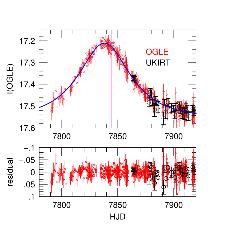
Figure 1: OGLE and UKIRT data for OGLE-2017-BLG-0173. The OGLE data (red) trace a seemingly normal low-amplitude microlensing event. The time interval of the anomaly, marked by a pair of magenta vertical lines, by chance does not overlap the periods of visibility from Chile. The black points show the UKIRT $H$-band data (transformed to the OGLE scale). Although these begin well after peak, they enable an $(I-H)$ color measurement.

Although the source is a low-luminosity giant, and therefore quite luminous relative to the majority of microlensed sources, it is also highly extincted, $A_{I}=2.8$. Hence, it is extremely faint in $V$ band. While many faint-$V$ sources nevertheless can ultimately yield very good $(V-I)$ colors (e.g., Yee et al. 2012), this is only because they are observed at high magnification. By contrast, the most highly magnified $V$ point for OGLE-2017-BLG-0173 has a magnification $A\sim 2.2$ (i.e., $\Delta A=1.2$ relative to baseline), which yields only very poor constraints on the source color. Fortunately, the UKIRT microlensing survey (Shvartzvald et al., 2017), which is primarily motivated to improve understanding of future WFIRST microlensing observations (Spergel et al., 2013), observed this field using the wide-field near infrared camera (WFCAM) with a nominal cadence of $\Gamma=1\,{\rm day}^{-1}$ in $H$-band. Although these observations began 26 days after peak, when the source was just leaving the Einstein ring (so magnified by only $\Delta A\sim 0.3$, see Figure 1), the source was quite bright in this passband, $H_{s}\sim 14.5$, which enables a good $(I-H)$ color measurement. See Section 4.1. The UKIRT/WFCAM images were reduced by the Cambridge Astronomy Survey Unit (CASU; Irwin et al. 2004). The UKIRT light curve was extracted using a soft-edged circular aperture and was photometrically calibrated to 2MASS (see Hodgkin et al. 2009 for details).

3 Analysis

The OGLE-2017-BLG-0173 light curve is comprised of a long low-amplitude hump, lasting several months which rises just 0.35 mag above baseline (see Figure 1), punctuated by a short $(<1\,{\rm day})$ bump, which rises an additional 0.3 mag (see Figure 2). The anomaly starts and ends with an abrupt rise and fall, indicating a caustic entrance and exit respectively. However, there is no “dip” between these, implying that the source must be larger than the separation between the two sides of the caustic. The simplest way to account for this behavior is that the source envelops a substantial fraction of, or perhaps the whole, caustic. While a few such events have previously been observed, e.g., OGLE-2005-BLG-390 (Beaulieu et al., 2006) and OGLE-2008-BLG-092 (Poleski et al., 2014a), there has never been a discussion of how to intuitively understand this generic class of events. We therefore begin with such a heuristic analysis.

3.1 Heuristic Analysis

In general, a minimum of six geometric parameters are required to describe a binary microlensing event: $(t_{0},u_{0},t_{\rm E},s,q,\alpha)$. The first three are the Paczyński (1986) parameters of the underlying event due to the system as a whole, i.e., the time of closest approach, the impact parameter (scaled to $\theta_{\rm E}$) and the Einstein timescale,

$$t_{\rm E}\equiv{\theta_{\rm E}\over\mu},$$ (3)

where $\mu$ is the lens-source relative proper motion and $\mu=|{\mbox{\boldmath$\mu$}}|$. For the case of planetary companions, particularly those of very low mass, the great majority of the light curve follows the standard Paczyński (1986) flux evolution:

$$F(t)=f_{s}A[u(t;t_{0},u_{0},t_{\rm E})]+f_{b};\qquad A(u)={u^{2}+2\over u\sqrt{u^{2}+4}};\qquad u^{2}={(t-t_{0})^{2}\over t_{\rm E}^{2}}+u_{0}^{2},$$ (4)

where $f_{s}$ is the source flux and $f_{b}$ is any blended light in the aperture not taking part in the event. The normalized separation $s$ and mass ratio $q$ have already been described, while $\alpha$ gives the direction of the star-planet axis relative to $\mu$. If the source passes over or close to any caustics, one must also specify a seventh parameter,

$$\rho\equiv{\theta_{*}\over\theta_{\rm E}},$$ (5)

where $\theta_{*}$ is the angular source radius.

As shown in Figure 1, the OGLE data are quite well fit by a standard Paczyński (1986) curve, Equation (4). After including the KMTNet data as well (but excluding the anomaly) we find that the Paczyński (1986) parameters are,

$$(t_{0},u_{0},t_{\rm E},f_{s},f_{b})=(7837.90,0.74,33.7\,{\rm day},0.93,0.61),\qquad({\rm point-lens\ fit}),$$ (6)

where the flux scale is set by $f\equiv 1$ at $I=18$. In addition to these five parameters, we must still evaluate the four others related to the planet that were defined above, $(s,\alpha,q,\rho)$. The first two of these are quite straightforward.

The perturbation is centered at $t_{\rm anom}=7844.3$, i.e., at $\tau_{\rm anom}\equiv(t_{\rm anom}-t_{0})/t_{\rm E}=0.190$. Hence, the position and orientation within the Einstein ring are

$$u_{\rm anom}=\sqrt{u_{0}^{2}+\tau_{\rm anom}^{2}}=0.76\qquad\alpha=\tan^{-1}{u_{0}\over\tau_{\rm anom}}=1.32\,{\rm radian}.$$ (7)

The physical origin of the caustic is that one of the two images created by the gravity of the host, at scaled positions $(u\pm\sqrt{u^{2}+4})/2$, is passing near the planet, with separation $s$ from the host. However, as shown by Gould & Gaucherel (1997), when a source envelops the caustics due to the “minor” image ($(u-\sqrt{u^{2}+4})/2$), it tends to generate zero excess magnification rather than the bump that is seen in Figure 2. Hence we derive,

$$\qquad s={u_{\rm anom}+\sqrt{u_{\rm anom}+4}\over 2}=1.45\ .$$ (8)

To evaluate the remaining two parameters $(q,\rho)$ by eye is more difficult. We begin by making the simplifying assumption that the source completely envelops the caustic and then discuss how the estimates are impacted if this assumption fails and the caustic is only partially enveloped.

Gould & Gaucherel (1997) showed that for the case of an $s>1$ planetary caustic, the excess magnification at peak for a source that is much larger than the planetary Einstein radius $\theta_{{\rm E},p}\equiv\sqrt{q}\theta_{\rm E}$ is

$$\Delta A={2q\over\rho^{2}}.$$ (9)

That is, $\Delta A$ is the same as it would be if the planet were an isolated point-lens.

The excess flux can be read off the light curve, which then (combined with $f_{s}$) yields the excess magnification,

$$\Delta A={10^{-0.4\,I_{\rm anom,peak}}-10^{-0.4\,I_{\rm anom,base}}\over 10^{-0.4\,I_{s}}}=0.67;\qquad{q\over\rho^{2}}={\Delta A\over 2}=0.33,$$ (10)

where $I_{\rm anom,peak}=16.94$ and $I_{\rm anom,base}=17.23$ .

In order to evaluate $q$, we must determine $\rho$. Working in the limit that the source is much larger than the planetary Einstein radius ($q/\rho^{2}\ll 1$), which is only marginally satisfied by Equation (10), and assuming that the source center passes directly over the caustic, then $\rho=t_{\rm fwhm}/2t_{\rm E}$, where $t_{\rm fwhm}=0.5\,$days, is the full width at half maximum of the bump. Under this assumption,

$$\rho={t_{\rm fwhm}\over 2t_{\rm E}}=0.0074;\qquad q={\Delta A\over 2}\rho^{2}={t_{\rm fwhm}^{2}\Delta A\over 8t_{\rm E}^{2}}=1.84\times 10^{-5}.$$ (11)

The above formalism is appropriate if the source fully envelops the caustic, which we dub “Cannae” events. However, qualitatively similar event morphologies will be generated if the source envelops only one flank of the caustic, which we call “von Schlieffen” events. As a representative of these, we consider the case that the limb of the source (rather than its center) passes directly over the center of the caustic. Then, the above argument gives us $q=\Delta A\rho^{2}$, which yields $q=3.7\times 10^{-5}$.

Hence, the heuristic analysis indicates that $10^{-5}\lesssim q\lesssim 10^{-4}$, but more detailed numerical analysis is needed to make a more precise estimate. More generally, this analysis tells us that planets of quite small mass ratio are easily detectable in these large-source events.

3.2 Numerical Analysis

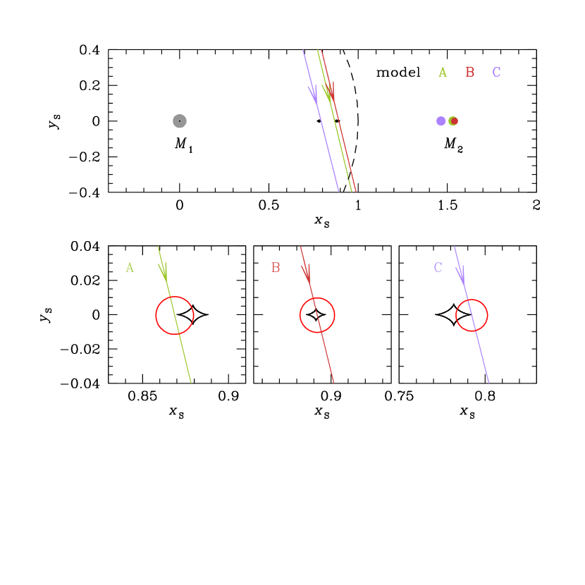
Figure 3: Geometries of the three models (A,B,C) of OGLE-2017-BLG-0173. The upper panel shows source trajectory and lens-component positions color coded by model as well as the location of the caustic. The zooms in the lower panel show that the giant-star source either partially (A,C) or fully (B) envelops the caustic, making this either a “von Schlieffen” or “Cannae” type “Hollywood” event.

To carry out a systematic analysis, we begin (as described above) by fitting a Paczyński (1986) curve to the full data set excluding the anomaly, in order to obtain initial estimates of $(t_{0},u_{0},t_{\rm E})$. We also make an initial estimate of $\rho=0.01$ following the reasoning above. We then conduct a grid search over $(s,q)$ space, holding these two parameters fixed and allowing the other five to vary, including $\alpha$ which we seed at a grid of values. We use inverse-ray shooting (Kayser et al., 1986; Schneider & Weiss, 1988; Wambsganss, 1997) when the source is close to a caustic and multipole approximations (Pejcha & Heyrovský, 2009; Gould, 2008) otherwise. We employ Monte Carlo Markov Chain (MCMC) to locate all minima. We find three solutions (A,B,C). All three have very similar geometries defined by $(t_{0},u_{0},t_{\rm E},\rho,s,\alpha)$, but one of them (B) has a Cannae topology and the other two have von Schlieffen topologies, one on each flank. Note that the degeneracy between solutions A and C was already predicted by Gaudi & Gould (1997), but the degeneracy of these two solutions with B has not previously been predicted nor seen in practice. Figure 2 shows the three model light curves superposed on the data, while Figure 3 shows the lens-source geometries and the resulting relations between the source and the caustics. The best fit parameters and uncertainties are shown in Table 1. Note that all of the parameters are in reasonable agreement with those derived from the heuristic analysis of Section 3.1. In particular, for the Cannae solution, the estimated mass ratio $q$ is too low by about 25% and for the von Schlieffen solutions it is too low by about 40%.

As demonstrated by Table 1, the three solutions are extremely close in terms of $(t_{0},u_{0},s,\alpha)$ geometry, but are strongly separated in $q$. We find that the three minima are discrete in the sense that the MCMC does not jump from one to the other in a normal run, showing that the barriers between them are too high. To explore the nature of these barriers, we run a “hotter” MCMC (artificially inflating the error bars by a factor 3.0 and then, to compensate for this, multiplying the resulting $\chi^{2}$ values by 9.0). To trace the relation between these solutions, we introduce the parameter

$$\Delta\xi\equiv u_{0}\csc\alpha-\xi_{+}(s);\qquad\xi_{+}(s)\equiv s-s^{-1},$$ (12)

where $[\xi_{+}(s),0]$ is the Einstein-ring position of the center of the major-image caustic for a planet in the regime $q\ll 1$ with separation $s$. That is, $\Delta\xi$ is the offset between the centers of the source and the caustic as the source crosses planet-star axis.

Figure 4 plots $\log q$ vs. $\Delta\xi$. It shows a broad minimum in $q$ centered near $\Delta\xi=0$ (solution B), with $q$ rising roughly symmetrically toward solutions A and C on either side. These tracks are continuous in the parameters of the plot, but have relatively high barriers between the three minima, as expected. We find that these barriers have heights of $\Delta\chi^{2}\sim 35$ between solutions A and B, and $\Delta\chi^{2}\sim 60$ between solutions B and C.

The $\chi^{2}$ differences between the best (B) and worst (C) solutions is $\Delta\chi^{2}\sim 16$, and hence solution C can be considered as strongly disfavored. However, the two von Schlieffen solutions (A and C) have almost identical physical implications, while solutions A and B have very similar $\chi^{2}$. Hence, the degeneracy between solutions with different $q$ (and so different physical implications) is quite severe.

3.3 Reality of Roughly Equal Source and Blend Fluxes?

A mildly peculiar feature of these solutions is that $f_{s}$ and $f_{b}$ are comparable. This is more true of solution C than either A or B. Nevertheless, this statement qualitatively describes all three solutions. Such rough equality is frequently observed for typical microlensed sources, which are most often stars near the turnoff. Since the projected density of stars of similar luminosity is very high toward the bulge, it is not at all uncommon to have more than one in a ground-based seeing disk. However, as we will discuss in Section 4.1, the “baseline object” is in or near the Galactic bulge clump, and it would be much rarer to have a star of comparable brightness projected on such a source. The issue is important because spurious blending could be an indication of systematic errors in the data that are driving the solution.

Fortunately, we have very clear evidence that the blending is real, which also permits us to estimate the allowed range of $f_{b}/f_{s}$ completely independent of the light curve analysis.

We find that the astrometric position of the “baseline object” (i.e., the cataloged “star” derived from analysis of the template image) is offset from the position of the source by $\Delta\theta_{\rm app}=0.13^{\prime\prime}$. The source position is derived by finding the position of the “difference star” formed by subtracting the template image from images taken near peak magnification. The offset between the blending star (or the light centroid of several blending stars) and the source, $\Delta\theta$, is related to the apparent offset by

$$\Delta\theta_{\rm app}={f_{b}\Delta\theta\over f_{s}+f_{b}}\qquad\Longrightarrow\qquad{f_{b}\over f_{s}}=\biggl{(}{\Delta\theta\over\Delta\theta_{\rm app}}-1\biggr{)}^{-1}$$ (13)

We consider that if the blend were separated by more than one FWHM in the very good seeing images of the template, FWHM$\sim 0.8^{\prime\prime}$, then it would have been separately resolved, i.e., $\Delta\theta\lesssim 0.8^{\prime\prime}$. Hence, Equation (13) implies: $0.19\lesssim f_{b}/f_{s}<\infty$. From Table 1, the best fit values for this ratio are $f_{b}/f_{s}=(0.34,0.28,0.60)$ for solutions (A,B,C), which are all easily satisfied. Alternatively, we can derive best fit estimates $\Delta\theta=(0.51^{\prime\prime},0.59^{\prime\prime},0.35^{\prime\prime})$. In all cases it is quite plausible that blends with the corresponding flux ratios would not be detected at these separations in the template.

3.4 Binary-Source Solution?

As pointed out by Gaudi (1998) short-term peaks that are the hallmark of planetary perturbations can also be generated by a second source, which then typically should pass very close to the lens (accounting for its short apparent timescale) and would then also be very faint (so as not to completely dominate the light curve during this close passage). We search for such solutions but do not find acceptable fits. See Figure 2. The basic reason for this is that the perturbation is simply too compact.

To better understand the underlying reasons for this numerical result, we first consider the case that the second source is not impacted by finite source effects. Then the effective timescale $t_{{\rm eff},2}\equiv u_{0,2}t_{\rm E}\simeq t_{\rm fwhm}/\sqrt{12}=0.14\,{\rm day}$, which implies that the excess flux during the Chile observations at $\Delta t=0.45\,{\rm day}$ would be $f_{\rm exc}=f_{2,\rm peak}/\sqrt{1+(\Delta t/t_{\rm eff})^{2}}\simeq 12^{-1/2}(t_{\rm fwhm}/\Delta t)f_{2,\rm peak}=0.2$, corresponding to a change of 0.1 magnitudes. This would clearly contradict the data.

On the other hand, consider the case that the second source passes directly over the lens. One may show that $t_{\rm fwhm}\simeq 2.2\,\rho t_{\rm E}$. Then $f_{s,2}=f_{2.\rm peak}\rho_{2}/2$, and hence the excess flux seen from Chile just before the bump would be $f_{\rm exc}=f_{s,2}t_{\rm E}/\Delta t=f_{2,\rm peak}t_{\rm fwhm}/4.4\Delta t=0.17$, corresponding to about 0.08 mag. This is still clearly excluded by the data.

4 Physical Parameters

The lens mass $M$ and lens-source relative parallax $\pi_{\rm rel}$ can in principle be determined provided that both the Einstein radius $\theta_{\rm E}$ (Equation (1)) and the microlens parallax (Gould, 1992, 2000; Gould & Horne, 2013),

$${\mbox{\boldmath$\pi$}}_{\rm E}\equiv{\pi_{\rm rel}\over\theta_{\rm E}}\,{{\mbox{\boldmath$\mu$}}\over\mu},$$ (14)

can be measured. Then, $M=\theta_{\rm E}/\kappa\pi_{\rm E}$ and $\pi_{\rm rel}=\theta_{\rm E}\pi_{\rm E}$. As in most planetary microlensing events, $\theta_{\rm E}$ can be measured, but unfortunately we find that ${\mbox{\boldmath$\pi$}}_{\rm E}$ can be neither measured nor meaningfully constrained. Therefore, after measuring $\theta_{\rm E}$ in Section 4.1, we apply a Galactic model to estimate the lens mass and distance.

4.1 Measurement of $\theta_{\rm E}$ and $\mu$

As mentioned in Section 2, we are able to roughly place the “baseline object” on a $[(V-I),I]$ color-magnitude diagram (CMD), but we cannot actually measure the source color in these bands. This is due partly to its faintness in $V$ (as a result of the $A_{V}\sim 5$ magnitudes of extinction), and partly because its peak magnification is quite modest. We therefore use UKIRT $H$ band in place of the usual $V$ band, to determine the color.

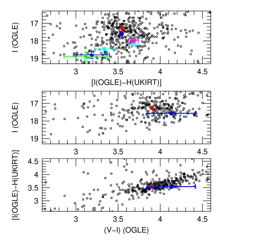
Figure 5: CMDs (in $(I-H)$ and $(V-I)$) and $VIH$ color-color diagram of field stars near OGLE-2017-BLG-0173, together with the positions of the clump centroid (red), the “baseline object” (blue), and for each of the three solutions (A=magenta, B=green, C=cyan), the source star (open circles), and the blended light (five-pointed stars). The “baseline object” is barely detected in $V$ band, which results in a 0.3 mag uncertainty in its color. Hence, we use an $[I,(I-H)]$ CMD (top panel) to determine the intrinsic source color. The offset between the source and the clump (in both color and magnitude), leads to an angular source radius $\theta_{*}=(5.30,5.43,4.86)\,\mu{\rm as}$, which is used to estimate the Einstein radius $\theta_{\rm E}=(0.48,0.54.53)\,{\rm mas}$ for solutions (A,B,C). See Section 4.1.

As illustrated in Figure 5, the source is $0.16\pm 0.06$ mag redder and for solutions (A,B,C) $(0.60,0.55,0.79)\pm(0.09,0.11,0.07)$ mag fainter than the clump in these bands. We use Bessell & Brett (1988) to convert the color offset to $\Delta(V-I)=0.13\pm 0.06$. Then adopting $[(V-I),I]_{0,\rm clump}=(1.06,14.43)$ from Bensby et al. (2013) and Nataf et al. (2013), we find $[(V-I),I]_{0,s}=[1.19,(15.03,14.98,15.22)]$. Again using the color-color relations of Bessell & Brett (1988) as well as the the color/surface-brightness relation of Kervella et al. (2004), we find,

$$\theta_{*}=(5.30,5.43,4.86)\pm(0.30,0.35,0.26)\,\mu{\rm as},$$ (15)

and so (taking account of the correlation between $\rho$ and $f_{s}$),

$$\theta_{\rm E}={\theta_{*}\over\rho}=(0.48,0.54,0.53)\pm 0.03\,{\rm mas};\quad\mu={\theta_{\rm E}\over t_{\rm E}}=(5.7,6.5,5.9)\pm(0.3,0.4,0.3)\,{\rm mas}\,{\rm yr}^{-1}.$$ (16)

4.2 Bayesian Estimate

The angular Einstein radius $\theta_{\rm E}$ and relative proper motion $\mu$ (Equation (16)) are quite consistent with either a disk or bulge lens. See upper left panel of Figure 7 of Penny et al. (2016). To make a more quantitative estimate of the lens characteristics, we draw lensing events randomly from a Han & Gould (1995, 2003) Galactic model and catalog the subset that are consistent with the observables, $\theta_{\rm E}$ and $\mu$.

The results are shown in Table 2. For host mass, system distance, and planet-host projected separation, the results are essentially the same for the three solutions: $M=0.39^{+0.40}_{-0.24}\,M_{\odot}$, $D_{L}=4.8^{+1.5}_{-1.8}\,{\rm kpc}$, and $a_{\perp}=3.8\pm 1.6\,{\rm AU}$. However, since $q$ is very different for the von Schlieffen solutions compared to the Cannae solution, the planet masses are also centered at very different values, $m_{p}=8\,M_{\oplus}$ and $m_{P}=3.3\,M_{\oplus}$, respectively. Since the fractional error in $q$ is much smaller than that of the Bayesian estimate of $M$, the fractional error in $m_{p}$ is dominated by the latter.

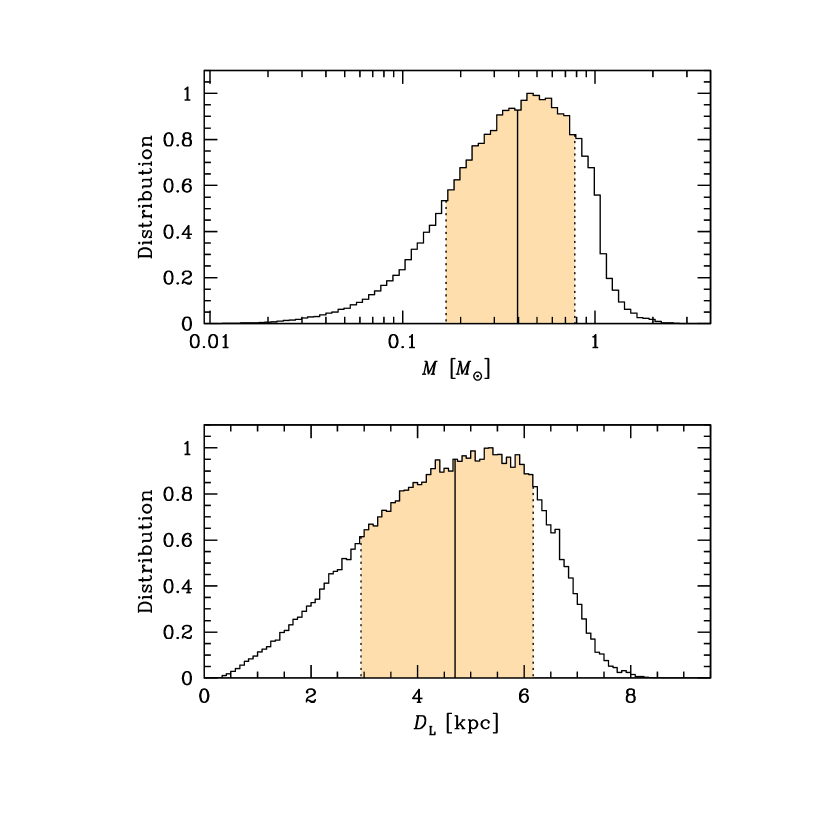
Figure 6: Histogram of posterior probabilities of the physical parameters of the lens system OGLE-2017-BLG-0173L, obtained by drawing event parameters from a Galactic model and comparing their observables $\theta_{\rm E}$ and $\mu$ with those derived from the microlensing light curve analysis. This histogram is for model B, but models A and C are virtually identical.

We show the posterior histograms for $M$ and $D_{L}$ for solution B in Figure 6. The corresponding figures for the other two solutions are extremely similar and so are not shown.

4.3 Future Resolution

Because of its low mass ratio, either $q\simeq 6.5\times 10^{-5}$ (solutions A and C) or $q\simeq 2.5\times 10^{-5}$ (solution B), it would be of significant interest to determine the true mass of the host and to resolve the degeneracies among the three solutions, and thereby determine the mass of the planet. Here we show that the first will eventually be possible and that the second will probably not be possible.

If the event had occurred somewhat later in the season, it could have been targeted for Spitzer microlensing observations (Gould et al., 2016). However, the first epoch at which it was visible by Spitzer was at HJD${}^{\prime}=7930$ when $u\sim 2.7$, and hence $A\sim 1.024$, i.e., quite close to baseline. Such observations were nevertheless attempted, but did not yield useful constraints.

Hence, the best hope for measuring the host mass is to image the lens when it has sufficiently separated from the source, using high-resolution imaging. Since the source is likely to be 100–1000 times brighter than the lens, it will probably require (with current instruments) about 1.5 times larger separation than the $60\,{\rm mas}$ separation by which Batista et al. (2015) resolved the roughly equal-brightness lens and source of OGLE-2005-BLG-169. From the measured proper motion, this would require a roughly 15 year wait. In the meantime, high-resolution imagers of next generation (“30 meter”) telescopes may come on line, in which case the lens could be imaged at first light.

To aid with these measurements, which may be decades in the future, we give a short summary of what is known from the event about the $H$-band fluxes and their errors together with the underlying reason. The most precise measurement is of the $(I-H)$ source color, where $I$ is in the OGLE-IV system and $H$ is in the 2MASS system: $(I-H)_{s}=3.71\pm 0.06$. This is essentially independent of any model and depends on regression and the assumption of achromaticity, which follows from general relativity. At the next level, we have $H_{s}=I_{s}-(I-H)_{s}=(14.14,14.09,14.34)\pm(0.11,0.12,0.09)$ for (A,B,C), where $(I-H)_{s}$ is described just above and the $I_{s}$ are derived from the models (see Table 1). Since the $I_{s}$ and $(I-H)_{s}$ measurements are essentially independent, the errors are added in quadrature. Finally, we report the $H$-band baseline $H_{\rm base}=14.01\pm 0.01$. Because there are enough data very close to baseline, the error in this quantity is basically just the calibration error. Therefore, subtracting fluxes and noting that the $H_{b}$ and $H_{s}$ flux errors are the same, we obtain $H_{b}=(16.37,16.88,15.46)\pm(0.86,1.56,0.25)$.

By directly resolving the host and measuring both its color and magnitude (and combining this with the mass-distance constraint from the measurement of $\theta_{\rm E}=\sqrt{\kappa M\pi_{\rm rel}}$), the host mass can be determined.

Unfortunately, such a measurement would not discriminate among the three solutions. All three predict similar lens masses and distances. This is particularly true of solution A and B, which differ by only $\Delta\chi^{2}=2.5$.

However, the same high-resolution imaging (or even a high resolution image taken much sooner) could in principle partially discriminate among solutions by separately resolving the source and the blended light. Suppose, for example, that the blended light were measured to have $I_{b}=19.0$, corresponding to $f_{b}=0.40$. From Table 1, this would be consistent with solutions A and B, but inconsistent with solution C. Unfortunately, solutions A and B predict the same $f_{b}$ to well within $1\,\sigma$ so there is no possibility of distinguishing between them by measuring $f_{b}$.

5 Discussion

5.1 Nature of Degeneracy

As just discussed in Section 4.3, the factor 2.5 degeneracy in the planet-host mass ratio between solutions A+C and solution B cannot be resolved from the existing data and may never be resolved. Hence, while there is no doubt that OGLE-2017-BLG-0173Lb is a very low mass-ratio planet $q<10^{-4}$, and may be the lowest yet detected $(q\simeq 2.5\times 10^{-5})$ its actual mass ratio remains somewhat uncertain. Given that the planetary deviation is detected with extremely high confidence $(\Delta\chi^{2}\sim 10,000)$, it is of considerable interest to understand the nature of the degeneracy.

Inspection of Figure 2 shows that this is an “accidental” degeneracy in that the model light curves differ significantly in regions of the anomaly where there are gaps in the data. These in turn are due to the fact the anomaly occurred quite early in the season (31 March), when KMTNet was able to observe only 4.0 hours from each site. In particular, models A and B are well separated during the $\sim 3.5\,$hrs prior to the onset of KMTA observations. While models B and C are less well separated, model C is already disfavored by $\Delta\chi^{2}=16$. Hence, it is likely that this degeneracy would have been resolved if the event had occurred, for example, 2 months later.

5.2 Poster Child for “Hollywood” Events

The mass ratio, $q\simeq 2.5\times 10^{-5}$ or $q\simeq 6.5\times 10^{-5}$, of OGLE-2017-BLG-0173 is among the lowest for any microlensing planet (see e.g., Figure 7 from Mróz et al. 2017). Yet the signal is quite strong. From the analysis given in Section 3.1, if $q$ had been substantially smaller, say $q=10^{-5}$, (and focusing for the moment on solution B), then the light curve would have looked qualitatively similar but with the amplitude of the bump, $\Delta A$, reduced by a factor of 2.7. In this case, it still would have been easily recognized. Moreover, the excess magnification would have been the same, regardless of the planet-host separation, provided $s>1$ and of course provided that the source passed over the caustic. For example, Poleski et al. (2014a) discovered a $q=2.4\times 10^{-4}$ planet from the passage of a giant source over an $s=5.26$ planetary caustic, with $\rho=0.04$, in OGLE-2008-BLG-092. Hence, $\Delta A=2q/\rho^{2}=0.3$, which is quite similar to the present case. In addition, Poleski et al. (2014b) found a $q=0.016$ companion from a giant source (very similar to the OGLE-2017-BLG-0173 source, with similar $\rho\sim 0.01$) passing over an outlying caustic, $s=4.4$, in MOA-2012-BLG-006. However, in this case, the large mass ratio implied that the companion Einstein radius was about 10 times larger than the source, so that $\Delta A\gg 1$, and hence the framework of Section 3.1 does not apply.

These facts illustrate the strengths of the “Hollywood strategy” advocated by Gould (1997) of “following the big stars” to find planets. Whenever the star is so big that it can envelop the caustic, the cross section for anomalous deviations from a Paczyński (1986) curve grows from the size of the caustic (or a bit more) to the size of the source. The duration of the deviation likewise grows, implying that modest-duration breaks in the light-curve coverage (like the ones before and after KMTA observations near HJD${}^{\prime}=7844$ in Figure 2) do not compromise the detection (although, as discussed in Section 5.1, they can degrade characterization).

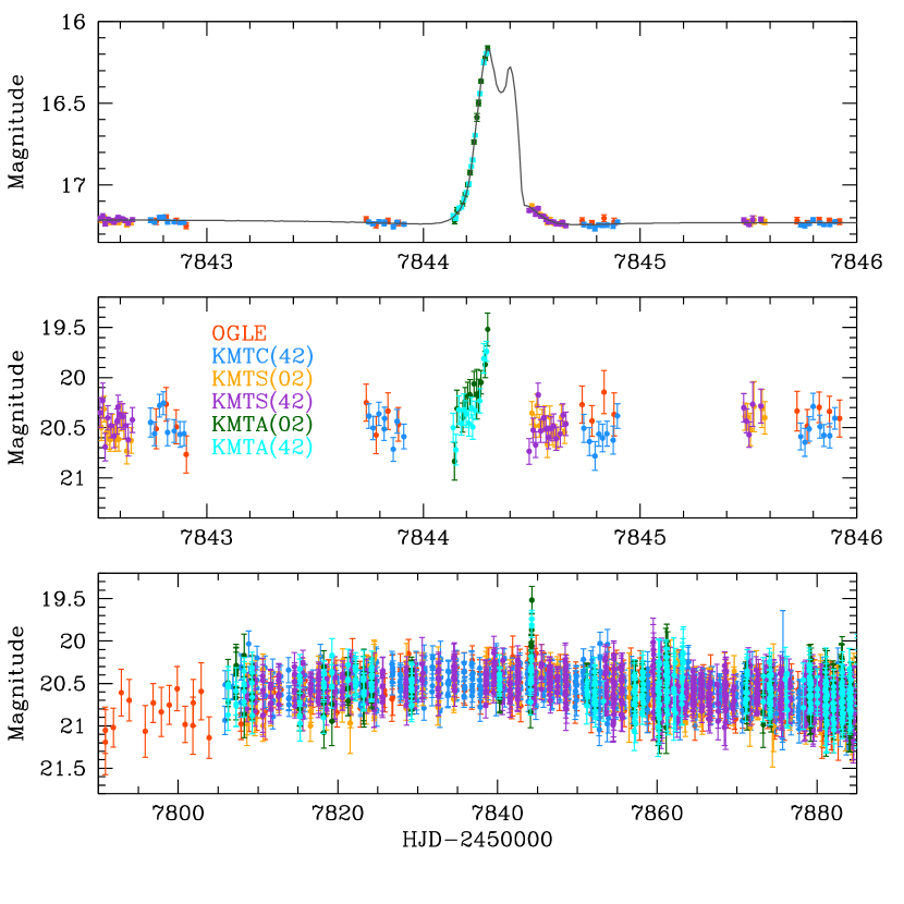
Figure 8: Dissection of the virtues of Hollywood through simulated data, illustrated for model B. Similarly to model A in Figure 7, the idealized upper panel would enable a well characterized planet but the more realistic middle panel (based on making the source not only smaller but correspondingly fainter) would not. Again, it is far from clear from the bottom panel that the underlying event would be recognized as microlensing.

To highlight these points, we show in Figures 7, 8 and  9, simulated events that are geometrically identical to the real one for models (A,B,C), except with a source that is 9.6 times smaller than the real source. For didactic purposes, the top panel in each Figure shows what the light curve would look like if the source had the same brightness, despite being much smaller. In this case, there are quite clear (A,B) or relatively clear (C) signatures of an anomaly. The difference between these two classes is simply the result of where the gaps fall relative to the strongest part of the anomaly.

The middle panel in each Figure shows a more realistic situation. The source is fainter by a factor of 20, similar to a bulge turnoff star. In this case, there is no recognizable anomaly at all for model C, and a only a suggestive hint of an anomaly for models A and B. In any case, it would not be possible to claim detection of a planet in any of the three cases.

The bottom panel in each figure shows the whole light curve. It is far from clear that the parent microlensing event would even be recognized in any of the three cases.

To construct the top panels of these figures, we used the original error bars from Figure 2, and we took the residuals from the zoom of Figure 2 and added these to each of the models shown. For the lower two panels, we multiplied both the error bars and residuals by a factor 10.

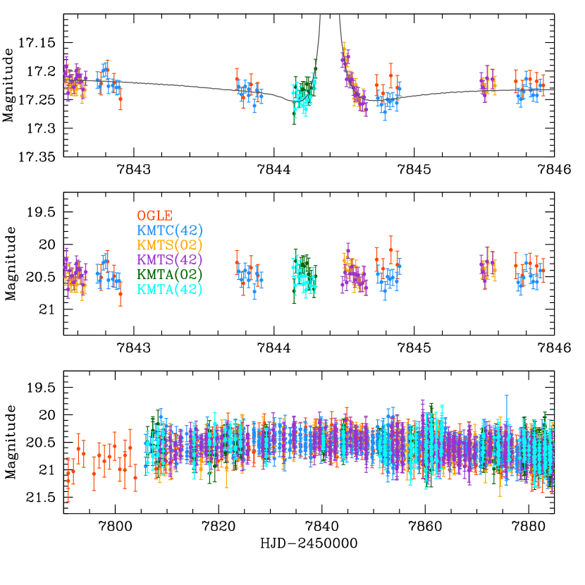
Figure 9: Dissection of the virtues of Hollywood through simulated data, illustrated for model C. Compared to models A (Figure 7) and B (Figure 8), the idealized upper panel is substantially less interprepretable due to the fact that, by chance, almost the entire bump lies in the data gap. Hence, in the more realistic middle panel, there is hardly a hint of the anomaly.

In creating the Hollywood moniker, Gould (1997) appears to have had in mind primarily events in which the caustic is fully enveloped by the source, in that he emphasized all three characteristics: larger cross-section, brighter sources, and longer duration. The classic example of such an event is OGLE-2005-BLG-390 (Beaulieu et al., 2006). However, one can also consider cases, like models A and C presented here, in which the source is comparable to the size of the caustic but only partially envelops it, as a second sub-class of Hollywood events. We have dubbed these sub-classes as “Cannae” and “von Schlieffen” events, respectively. Comparing Figures 7, 8, and 9 with each other and with Figure 2, one sees that the latter are still of the “Hollywood”-type in that they retain the properties of greater source brightness and longer duration. Thus, the range of such events is larger than that originally proposed by Gould (1997). Because the probability of detecting a planet in such an event scales much less strongly with mass ratio than for a typical source, Hollywood events can play a crucial role in the detection and characterization of planets, in particular those of low mass.

Hollywood events do have their drawbacks. Bennett & Rhie (1996) showed that the signal from Earth/Sun mass-ratio planets will be almost completely “washed out” by giant sources. On the other hand, Jung et al. (2014), taking account of the higher precision measurements from giant sources, argued that Earth-mass planets would be more detectable than for smaller sources (except for separations $s\sim 1$). This tension can be illustrated in the present case by noting from Section 3.1 that such a $q=3\times 10^{-6}$ planet would generate a $\Delta A=2q/\rho^{2}=0.06$ bump in a fully-enveloped, Cannae event (model B). The probability for envelopment would be a factor 10 larger than for a caustic crossing for a typical, turn-off star, microlensing source. However, while such a bump would certainly be detectable in the present data, whether it could be unambiguously interpreted is less clear.

In any case, the range of $q$ that is accessible to this approach extends at least a factor 5 below the previous lowest values, even if it does not reach the Earth/Sun regime.

Another potential drawback of Hollywood is the degeneracy discovered in this paper between Cannae and von Schlieffen solutions. Although this degeneracy was shown to be “accidental” in the sense that it was due to data gaps, such gaps are likely to be common. Furthermore, this degeneracy is present despite the $\Delta\chi^{2}\sim 10,000$ detection of the planet. We therefore investigated the case of OGLE-2005-BLG-390 (Beaulieu et al., 2006), which was the first Hollywood planet. We find that while the analog of Figure 4 shows the same “U” shaped structure, it does not contain multiple minima. Hence, there is no degeneracy despite the fact that the planet is detected at only $\Delta\chi^{2}\sim 500$. Noting that the source is much larger than the caustic in the case of OGLE-2005-BLG-390, we conjecture that this is the decisive difference. That is, we suggest that the degeneracy found in OGLE-2017-BLG-0173 will occur primarily in events for which the source and caustic have similar size.

When the “Hollywood strategy” was proposed, it was indeed a “strategy” in the sense that one had to choose to which targets one should apply limited follow-up resources. By contrast, OGLE-2017-BLG-0173Lb was discovered in pure survey mode, in which no decisions were needed or made about individual targets. However, the problem of applying limited follow-up telescope resources does continue to apply to Spitzer microlensing, and after the planetary nature of OGLE-2017-BLG-0173 was recognized, the Spitzer team (Gould et al., 2016) revised their selection strategy to give much greater emphasis to Hollywood events. More generally, there remains the question of how to apply limited human resources. We suggest that searches for smooth bumps, even of quite low amplitude, in current light curves and archival microlensing events with giant sources, may yield low-mass outlying planets that have not previously been recognized.

Table 1: Best-fit Solution

Parameters	model A	model B	model C
$\chi^{2}/\rm{dof}$	7445.54/7443	7442.07/7443	7458.08/7443
$t_{0}$ $(\rm{HJD}^{\prime})$	7838.031$\pm$0.059	7837.946$\pm$0.059	7838.011$\pm$0.059
$u_{0}$	0.844$\pm$0.035	0.867$\pm$0.043	0.768$\pm$0.028
$t_{\rm E}$ $(\rm{days})$	30.818$\pm$0.898	30.460$\pm$1.040	32.930$\pm$0.846
$s$	1.532$\pm$0.025	1.540$\pm$0.031	1.465$\pm$0.019
$q$ $(10^{-5})$	6.386$\pm$1.001	2.479$\pm$0.242	6.788$\pm$0.729
$\alpha$ $(\rm{rad})$	1.334$\pm$0.004	1.332$\pm$0.004	1.324$\pm$0.003
$\rho$ $(10^{-3})$	10.969$\pm$0.469	10.024$\pm$0.512	9.150$\pm$0.331
$F_{s}$	1.144$\pm$0.093	1.198$\pm$0.119	0.957$\pm$0.064
$F_{b}$	0.391$\pm$0.093	0.337$\pm$0.119	0.578$\pm$0.064

Table 2: Physical properties

Quantity	model A	model B	model C
$M_{\rm host}$ $[M_{\sun}]$	$0.357_{-0.208}^{+0.360}$	$0.396_{-0.227}^{+0.390}$	$0.396_{-0.229}^{+0.386}$
$M_{\rm planet}$ $[M_{\earth}]$	$7.581_{-4.911}^{+10.045}$	$3.269_{-2.015}^{+3.849}$	$8.950_{-5.585}^{+10.626}$
$D_{\rm L}$ [kpc]	$5.015_{-1.848}^{+1.463}$	$4.705_{-1.763}^{+1.468}$	$4.800_{-1.793}^{+1.463}$
$a_{\bot}$ [AU]	$3.688_{-1.540}^{+1.456}$	$3.913_{-1.649}^{+1.615}$	$3.727_{-1.553}^{+1.478}$

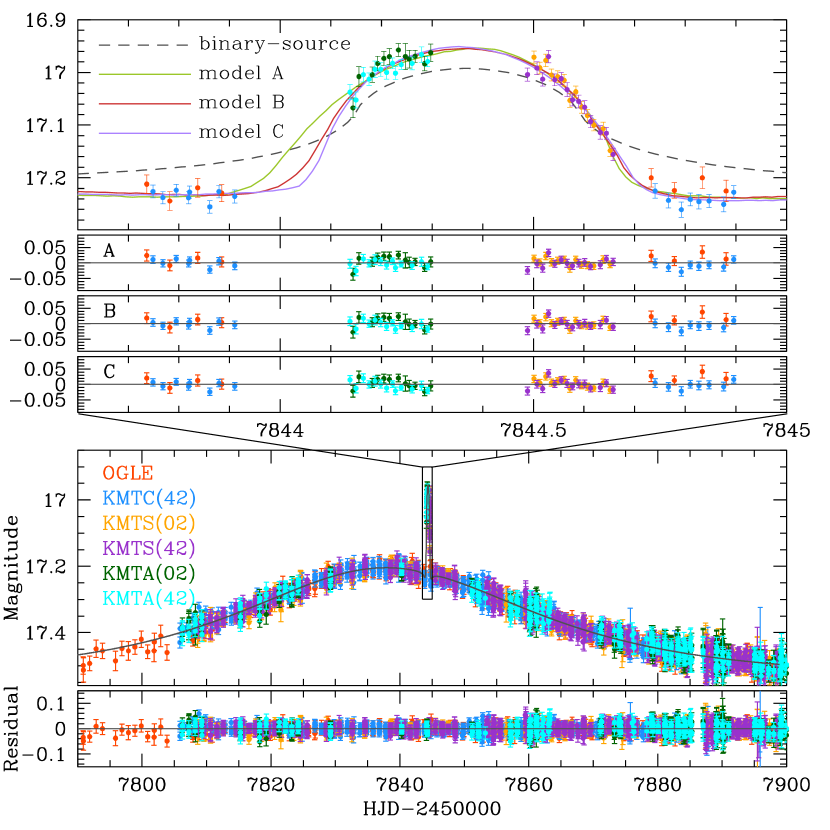
Figure 2: Light curve and models of OGLE-2017-BLG-0173. The short anomaly at HJD${}^{\prime}=7844.3$ on an otherwise perfectly normal point-lens Paczyński (1986) curve is due to a planet with mass ratio either $q\simeq 2.5\times 10^{-5}$ (model B) or $q\simeq 6.5\times 10^{-5}$ (models A and C). The upper panel is a zoom and also includes the best-fit binary-source model, which clearly fails to account for the data.

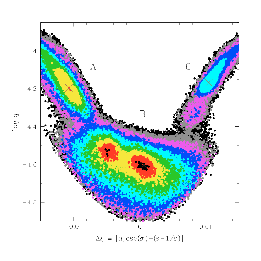
Figure 4: Scatter plot of MCMC of $\Delta\xi\equiv u_{0}\csc\alpha-(s-s^{-1})$ vs. $\log q$, where $\Delta\xi$ is the offset of the center of the source from the center of the caustic at the moment that the source crosses the binary axis, and $q$ is the mass ratio. The plot is derived primarily from a “hot chain”, to enable the sampling to cross the $\Delta\chi^{2}$ barriers between the three local minima, which we find to be $\Delta\chi^{2}\sim 35$ between models A and B, and $\Delta\chi^{2}\sim 60$ between models B and C. However, points from a normal-temperature chain are added to better articulate the minima. Color coding is (black, red, yellow, green, cyan, blue, magenta, gray) for $\Delta\chi^{2}<(1,4,9,16,25,36,49,64)$. Values of $\Delta\chi^{2}>64$ are again plotted in black.

Figure 7: Dissection of the virtues of Hollywood through simulated data, illustrated for model A. The upper panel shows how OGLE-2017-BLG-0173 would appear if the source had the same brightness but were 9.6 times smaller, i.e., similar to typical turnoff star microlensing sources. The source passes over the tip of the cusp, and becomes highly magnified, the rise of which is well-captured by KMTA data. In this idealization, the event would be well characterized. However, the middle panel shows a more realistic version, in which the source is not only smaller but also 20 times fainter. There is only a hint of an anomaly, and this certainly could not be characterized. Indeed, from the bottom panel, it is far from clear that the microlensing event due to the host star would even be recognized.

References

- Afonso et al. (2001) Afonso, C., Albert, J. N., Anderson, J. et al., 2001, A&A, 378, 1014
- Alard & Lupton (1998) Alard, C. & Lupton, R. H., 1998, ApJ, 503, 325
- Albrow et al. (2009) Albrow, M. D., Horne, K., Bramich, D. M., et al. 2009, MNRAS, 397, 2099
- Batista et al. (2015) Batista, V., Beaulieu, J.-P., Bennett, D. P., et al. 2015, ApJ, 808, 170
- Beaulieu et al. (2006) Beaulieu, J.-P. Bennett, D. P., Fouqué, P. et al. 2006, Nature, 439, 437
- Bennett & Rhie (1996) Bennett, D. P. & Rhie, S.-H. 1996, ApJ, 472, 660
- Bensby et al. (2013) Bensby, T. Yee, J. C., Feltzing, S. et al. 2013, A&A, 549A, 147
- Bessell & Brett (1988) Bessell, M. S., & Brett, J. M. 1988, PASP, 100, 1134
- Chang & Refsdal (1984) Chang, K. & Refsdal, S. 1984, A&A, 130, 157
- Chung et al. (2017) Chung, S.-J., Zhu, W., Udalski, A., 2017, ApJ, 838, 154
- Gaudi (1998) Gaudi, B. S. 1998, ApJ, 506, 533
- Gaudi (2012) Gaudi, B. S. 2012, ARA&A, 50, 411
- Gaudi & Gould (1997) Gaudi, B. S. & Gould, A. 1997, ApJ, 486, 85
- Gould (1992) Gould, A. 1992, ApJ, 392, 442
- Gould (1997) Gould, A. 1997, The Hollywood Strategy for Microlensing Detection of Planets, in Variables Stars and the Astrophysical Returns of the Microlensing Surveys. Eds. R. Ferlet, J.-P. Maillard and B. Raban. Gif-sur-Yvette, France : Editions Frontieres, p.125
- Gould (2000) Gould, A. 2000, ApJ, 542, 785
- Gould (2008) Gould, A. 2008, ApJ, 681, 1593
- Gould & Gaucherel (1997) Gould, A. & Gaucherel. 1997, ApJ, 477, 580
- Gould & Horne (2013) Gould, A. & Horne, K. 2013, ApJ, 779, L28
- Gould & Loeb (1992) Gould, A. & Loeb, A. 1992, ApJ, 396, 104
- Gould et al. (2016) Gould, A., Yee, J., & Carey, S., 2016, 2015spitz.prop.13005
- Gould et al. (2010) Gould, A., Dong, S., Gaudi, B.S. et al. 2010, ApJ, 720, 1073
- Griest & Safizadeh (1998) Griest, K. & Safizadeh, N. 1998, ApJ, 500, 37
- Han & Gould (1995) Han, C. & Gould, A. 1995, ApJ, 447, 53
- Han & Gould (2003) Han, C. & Gould, A. 2003, ApJ, 592, 172
- Henderson et al. (2014) Henderson, C. B., Gaudi, B. S., Han, C., et al. 2014, ApJ, 794, 52
- Hodgkin et al. (2009) Hodgkin, S. T., Irwin, M. J., Hewett, P. C., & Warren, S. J. 2009, MNRAS, 394, 675
- Irwin et al. (2004) Irwin, M. J., Lewis, J., Hodgkin, S., et al. 2004, Proc. SPIE, 5493, 411
- Jung et al. (2014) Jung, Y. K., Park, H., Han, C., et al. 2014 ApJ, 786, 85
- Kayser et al. (1986) Kayser, R., Refsdal, S., & Stabell, R. 1986, A&A, 166, 36
- Kervella et al. (2004) Kervella, P., Thévenin, F., Di Folco, E., & Ségransan, D. 2004, A&A, 426, 297
- Kim et al. (2016) Kim, S.-L., Lee, C.-U., Park, B.-G., et al. 2016, JKAS, 49, 37
- Mao & Paczyński (1991) Mao, S. & Paczyński, B. 1991, ApJ, 374, 37
- Mróz et al. (2017) Mróz, P., Han, C., Udalski, A. et al. 2017, AJ, 153, 143
- Nataf et al. (2013) Nataf, D. M., Gould, A., Fouqué, P. et al. 2013, ApJ, 769, 88
- Paczyński (1986) Paczyński, B. 1986, ApJ, 304, 1
- Pejcha & Heyrovský (2009) Pejcha, O., & Heyrovský, D. 2009, ApJ, 690, 1772
- Penny et al. (2016) Penny, M. T., Henderson, C.B., & Clanton, C. 2016, ApJ, 830, 150
- Poleski et al. (2014a) Poleski, R., Skowron, J., Udalski, A., et al. 2014a, ApJ, 755, 42
- Poleski et al. (2014b) Poleski, R., Udalski, A., Dong, S. et al. 2014b, ApJ, 782, 47
- Poleski et al. (2014b) Poleski, R., Udalski, A., Bond, I. A.. et al. 2017, A&A, 604A, 103
- Rattenbury et al. (2002) Rattenbury, N. J., Bond, I. A., Skuljan, J., & Yock, P. C. M. 2002, MNRAS, 335, 159
- Schneider & Weiss (1988) Schneider, P., & Weiss, A. 1988, ApJ, 330, 1
- Shvartzvald et al. (2014) Shvartzvald, Y., Maoz, D., Kaspi, S. et al. 2014, MNRAS, 439, 604
- Shvartzvald et al. (2017) Shvartzvald, Y.,Bryden, G., Gould, A., et al. 2017, AJ, 153, 61
- Spergel et al. (2013) Spergel, D. N., Gehrels, N., Breckinridge, J., et al. 2013, arXiv:1305.5422
- Sumi et al. (2016) Sumi, T., Udalski, A., Bennett, D. P., et al. 2016 ApJ, 825, 112
- Tsapras et al. (2014) Tsapras, Y., Choi, J.-Y., Street, R.-A., et al. 2014, ApJ, 782, 48
- Udalski (2003) Udalski, A. 2003, Acta Astron., 53, 291
- Udalski et al. (1994) Udalski, A., Szymanski, M., Kaluzny, J., Kubiak, M., Mateo, M., Krzeminski, W., & Paczyński, B. 1994, Acta Astron., 44, 317
- Udalski et al. (2015) Udalski, A., Szymański, M. K, & Szymański, G, 2015, Acta Astron., 65, 1
- Wambsganss (1997) Wambsganss, J. 1997, MNRAS, 284, 172
- Woźniak (2000) Woźniak, P. R. 2000, Acta Astron., 50, 421
- Yee et al. (2012) Yee, J. C., Shvartzvald, Y., Gal-Yam, A. et al. 2012, ApJ, 755, 102