First microlens mass measurement:
PLANET photometry of EROS BLG-2000-5

Abstract

We analyze PLANET photometric observations of the caustic-crossing binary-lens microlensing event, EROS BLG-2000-5, and find that modeling the observed light curve requires incorporation of the microlens parallax and the binary orbital motion. The projected Einstein radius ($\tilde{r}_{\rm E}=3.61\pm 0.11\ \mbox{AU}$) is derived from the measurement of the microlens parallax, and we are also able to infer the angular Einstein radius ($\theta_{\rm E}=1.38\pm 0.12\ \mbox{mas}$) from the finite source effect on the light curve, combined with an estimate of the angular size of the source given by the source position in a color-magnitude diagram. The lens mass, $M=0.612\pm 0.057\ \mbox{M}_{\sun}$, is found by combining these two quantities. This is the first time that parallax effects are detected for a caustic-crossing event and also the first time that the lens mass degeneracy has been completely broken through photometric monitoring alone. The combination of $\tilde{r}_{\rm E}$ and $\theta_{\rm E}$ also allows us to conclude that the lens lies in the near side of the disk, within $2.6\ \mbox{kpc}$ of the Sun, while the radial velocity measurement indicates that the source is a Galactic bulge giant.

1 Introduction

Although an initial objective of microlensing experiments was to probe the mass distribution of compact sub-luminous objects in the Galactic halo (Paczyński, 1986), the determination of the individual lens masses was in general believed not to be possible because the only generically measurable quantity is a degenerate combination of the mass with lens-source relative parallax and proper motion. However, Gould (1992) showed that there are additional observables that in principle can be used to break the degeneracy between physical parameters and so yield a measurement of the lens mass. If one independently measures the angular Einstein radius, $\theta_{\rm E}$, and the projected Einstein radius, $\tilde{r}_{\rm E}$:

$$\theta_{\rm E}\equiv\left(\frac{2R_{\rm sch}}{D_{\rm rel}}\right)^{1/2}\,;\ \ \ \tilde{r}_{\rm E}\equiv\left(2R_{\rm sch}D_{\rm rel}\right)^{1/2}\,,$$ (1)

then the lens mass $M$ is obtained by

$$M = \frac{c^{2}}{4G}\tilde{r}_{\rm E}\theta_{\rm E}$$ (2)

$$= 0.1227\ \mbox{M${}_{\sun}$}\left(\frac{\tilde{r}_{\rm E}}{1\ \mbox{AU}}\right)\left(\frac{\theta_{\rm E}}{1\ \mbox{mas}}\right)\ .$$

Here $R_{\rm sch}\equiv 2GMc^{-2}$ is the Schwarzschild radius of the lens mass, $D_{\rm rel}^{-1}=D_{\rm L}^{-1}-D_{\rm S}^{-1}$, and $D_{\rm L}$ and $D_{\rm S}$ are the distances to the lens and the source.

Measurement of $\theta_{\rm E}$ requires a standard ruler on the plane of the sky to be compared with the Einstein ring. For the subset of microlensing events in which the source passes very close to or directly over a caustic (region of singularity of the lens mapping at which the magnification for a point source is formally infinite), the finite source size affects the light curve. The source radius in units of the Einstein radius, $\rho_{\ast}$, can then be determined through analysis of the light curve, and thus, one can determine $\theta_{\rm E}$ ($=\theta_{\ast}/\rho_{\ast}$) once the angular radius of the source, $\theta_{\ast}$, is estimated from its de-reddened color and apparent magnitude. Although this idea was originally proposed for point-mass lenses, which have point-like caustics (Gould, 1994; Nemiroff & Wickramasinghe, 1994; Witt & Mao, 1994), in practice it has been used mainly for binary lenses, which have line-like caustics and hence much larger cross sections (Alcock et al., 1997, 2000; Albrow et al., 1999a, 2000a, 2001a; Afonso et al., 2000).

All ideas proposed to measure $\tilde{r}_{\rm E}$ are based on the detection of parallax effects (Refsdal, 1966; Grieger, Kayser, & Refsdal, 1986; Gould, 1992, 1995; Gould, Miralda-Escudé, & Bahcall, 1994; Hardy & Walker, 1995; Holz & Wald, 1996; Honma, 1999; An & Gould, 2001): either measuring the difference in the event as observed simultaneously from two or more locations, or observing the source from a frame that accelerates substantially during the course of the event. The prime example of the latter is the Earth’s orbital motion (annual parallax). For these cases, it is convenient to re-express $\tilde{r}_{\rm E}$ as the microlens parallax, ${\pi}_{\rm E}$,

$$\pi_{\rm E}\equiv\frac{\pi_{\rm L}-\pi_{\rm S}}{\theta_{\rm E}}=\frac{\mbox{1-kpc}/D_{\rm rel}}{\theta_{\rm E}/\mbox{1-mas}}=\frac{1\ \mbox{AU}}{\tilde{r}_{\rm E}}\ .$$ (3)

Here, $\pi_{\rm L}$ and $\pi_{\rm S}$ are the (annual) trigonometric parallax of the lens and the source so that $\pi_{\rm X}/\mbox{1-mas}=\mbox{1-kpc}/D_{\rm X}$, where subscript ‘X’ is either ‘L’(ens) or ‘S’(ource). To date, $\pi_{\rm E}$ has been measured for several events by detecting the distortion in the light curve due to the annual parallax effect (Alcock et al., 1995; Mao, 1999; Soszyński et al., 2001; Bond et al., 2001; Smith, Mao, & Woźniak, 2001; Mao et al., 2002; Bennett et al., 2001)

An & Gould (2001) argue that $\pi_{\rm E}$ is measurable for a caustic-crossing binary event exhibiting a well-observed peak caused by a cusp approach in addition to the two usual caustic crossings. Hence, one can determine the lens mass for such an event, since $\theta_{\rm E}$ can be estimated from any well-observed caustic crossing. The caustic-crossing binary event EROS BLG-2000-5 is archetypal of such events. In addition, the event has a relatively long time scale ($t_{\rm E}\sim 100\ \mbox{days}$), which is generally favorable for the measurement of $\pi_{\rm E}$.

In fact, EROS BLG-2000-5 features many unique characteristics not only in the intrinsic nature of the event but also in the observations of it. These include a moderately well-covered first caustic crossing (entrance), a timely prediction – of not only the timing but also the duration – of the second caustic crossing (exit), the unprecedented four-day length of the second crossing, and two time-series of spectral observations of the source during the second crossing (Albrow et al., 2001b; Castro et al., 2001). To fully understand and utilize this wealth of information, however, requires detailed quantitative modeling of the event. Here, we present the first model of EROS BLG-2000-5 based on the photometric observations made by the Probing Lensing Anomalies NETwork (PLANET) collaboration. In the current paper, we focus on the geometry of the event and find that both parallax and projected binary orbital motion are required to successfully model the light curve. Furthermore, we also measure the angular Einstein radius from the finite source effect during caustic crossings and the source angular size derived from the source position in a color-magnitude diagram (CMD). Hence, this is the first event for which both $\tilde{r}_{\rm E}$ and $\theta_{\rm E}$ are measured simultaneously and so for which the lens mass is unambiguously measured.

2 Data

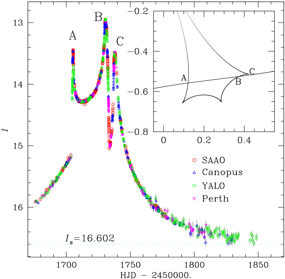
Figure 1: PLANET $I$-band light curve of EROS BLG-2000-5 (the 2000 season only). Only the data points used for the analysis (“cleaned high-quality” subset; see § 2) are plotted. Data shown are from SAAO (red circles), Canopus (blue triangles), YALO (green squares), and Perth (magenta inverted triangles). All data points have been de-blended using the fit result – also accounting for the seeing correction – and transformed to the standard $I$ magnitude; $I=I_{\rm s}-2.5\ \log[(F(t)-F_{\rm b})/F_{\rm s}]$. The calibrated source magnitude ($I_{\rm s}=16.602$) is shown as a dotted line. The three bumps in the light curve and the corresponding positions relative to the microlens geometry are also indicated.

On 2000 May 5, the Expérience de Recherche d’Objets Sombres (EROS) collaboration issued an alert that EROS BLG-2000-5 was a probable microlensing event ($\mbox{RA}=17^{\rm h}53^{\rm m}11\fs 5$, $\mbox{Dec}=-30\arcdeg 55\arcmin 35\arcsec$; $l=359\fdg 14$, $b=-2\fdg 43$). On 2000 June 8, the Microlensing Planet Search (MPS) collaboration issued an anomaly alert, saying that the source had brightened by 0.5 mag from the previous night and had continued to brighten by 0.1 mag in 40 minutes. PLANET intensified its observations immediately, and has been continuing to monitor the event up to the present (2001 August). Observations for PLANET were made from four telescopes: the Canopus 1 m near Hobart, Tasmania, Australia; the Perth/Lowell 0.6 m at Bickley, Western Australia, Australia; the Elizabeth 1 m at the South African Astronomical Observatory (SAAO) at Sutherland, South Africa; and the Yale/AURA/Lisbon/OSU (YALO) 1 m at the Cerro Tololo Interamerican Observatory (CTIO) at La Serena, Chile. Data were taken in $V$ (except Perth), $I$ (all four sites), and $H$ (SAAO and YALO) bands. For the present study, we make use primarily of the $I$ band data. That is, we fit for the model using only $I$ band data, while the $V$ band data are used (together with the $I$ data) only to determine the position of the source on CMD (see § 5). The light curve (Fig. 1) exhibits two peaks that have the characteristic forms of an entrance (A) and exit (B) caustic crossing (Schneider, Ehlers, & Falco, 1992, also see fig. 1 of Gould & Andronov 1999) immediately followed by a third peak (C) which is caused by the passage of the source close to a cusp.

The data have been reduced in a usual way and the photometry on them has been performed by point spread function (PSF) fitting using DoPHOT (Schechter, Mateo, & Saha, 1993). The relative photometric scaling between the different telescopes is determined as part of the fit to the light curve which includes the independent determinations of the source and the background fluxes at each telescope. We find, as was the case for several previous events, that due to the crowdedness of the field, the moderate seeing conditions, and possibly some other unidentified systematics, the amount of blended light entering the PSF is affected by seeing, and that the formal errors reported by DoPHOT tend to underestimate the actual photometric uncertainties. We tackle these problems by incorporating a linear seeing correction for the background flux and rescaling the error bars to force the reduced $\chi^{2}$ of our best model to unity. For details of these procedures, see Albrow et al. (2000a, b, 2001a) and Gaudi et al. (2002).

We also analyze the data by difference imaging, mostly using ISIS (Alard, 2000). We compare the scatter of the photometry on the difference images to that of the direct PSF fit photometry by deriving the normalized-summed squares of the signal-to-noise ratios:

$${\mathcal{Q}}\equiv\sum_{i}\left(\frac{F_{\rm s}A_{i}}{\tilde{\sigma}_{i}}\right)^{2}=\frac{N}{\chi^{2}}\sum_{i}\left(\frac{F_{\rm s}A_{i}}{\sigma_{i}}\right)^{2}\,,$$ (4)

where $F_{\rm s}$ is the source flux derived from the model, $A_{i}$ is the magnification predicted by the model for the data point, $\sigma_{i}$ and $\tilde{\sigma}_{i}$ are the photometric uncertainty (in flux) for individual data before and after rescaling the error bars [i.e. $\tilde{\sigma}_{i}=\sigma_{i}(\chi^{2}/N)^{1/2}$], and $N$ is the number of the data points. Strictly speaking, ${\mathcal{Q}}$ defined as in equation (4) is model-dependent, but if the data sets to be compared do not differ with one another in systematic ways (and the chosen model is close enough to the real one), ${\mathcal{Q}}$ can be used as a proxy for the relative statistical weight given by the data set without notable biases. We find that difference imaging significantly improves the stability of the photometry for the data from Canopus and Perth, but it somewhat worsens the photometry for the data from SAAO and YALO. We suspect that the result is related to the overall seeing condition for the specific site, but a definite conclusion will require more detailed study and would be beyond the scope of the current paper. We hope to be able to further improve the photometry on difference images in the future, but for the current analysis, we choose to use the data set with the better ${\mathcal{Q}}$ so that only for Canopus and Perth data sets, we replace the result of the direct PSF photometry with the difference imaging analysis result.

For the final analysis and the results reported here, we have used only a “high quality” subset of the data. Prior to any attempt to model the event, we first exclude various faulty frames and problematic photometry reported by the reduction/photometry software. In addition, data points exhibiting large (formal) errors and/or poor seeing compared to the rest of the data from the same site are eliminated prior to the analysis. In particular, the thresholds for the seeing cuts are chosen at the point where the behavior of “seeing-dependent background” becomes noticeably non-linear with the seeing variation. The criterion of the seeing and error cut for each data set is reported in Table 1 together with other photometric information. In conjunction with the proper determination of the error rescaling factors, we also remove isolated outliers as in Albrow et al. (2001a). Following these steps, the “cleaned high-quality” $I$-band data set consists of 1286 (= 403 SAAO + 333 Canopus + 389 YALO + 161 Perth) measurements made during the 2000 season (between May 11 and November 12) plus 60 additional observations (= 25 SAAO + 35 YALO) made in the 2001 season. Finally, we exclude 49 data points (= 19 SAAO + 20 Canopus + 10 Perth) that are very close to the cusp approach [$2451736.8<$ Heliocentric Julian Date (HJD) $<2451737.6$] while we fit the light curve. We find that the limited numerical resolution of the source, which in turn is dictated by computational considerations, introduces errors in the evaluation of $\chi^{2}$ in this region of the order of a few, and in a way that does not smoothly depend on the parameters. These would prevent us from finding the true minimum, or properly evaluating the statistical errors. However, for the final model, we evaluate the predicted fluxes and residuals for these points. As we show in § 4, these resdiuals do not differ qualitatively from other residuals to the fit.

3 Parameterization

To specify the light curve of a static binary event with a rectilinear source trajectory requires seven geometric parameters: $d$, the binary separation in units of $\theta_{\rm E}$; $q$, the binary mass ratio; $\alpha$, the angle of the source-lens relative motion with respect to the binary axis; $t_{\rm E}$, the Einstein timescale (the time required for the source to transit the Einstein radius); $u_{0}$, the minimum angular separation between the source and the binary center – either the geometric center or the center of mass – in units of $\theta_{\rm E}$; $t_{0}$, the time at this minimum; $\rho_{\ast}$, the source size in units of $\theta_{\rm E}$. (In addition, limb-darkening parameters for each wave band of observations, and the source flux $F_{\rm s}$ and background flux $F_{\rm b}$ for each telescope and wavelength band are also required to transform the light curve to a specific photometric system.) Most generally, to incorporate the annual parallax and the projection of binary orbital motion into the model, one needs four additional parameters. However, their inclusion, especially of the parallax parameters, is not a trivial procedure, since the natural coordinate basis for the description of the parallax is the ecliptic system while the binary magnification pattern possesses its own preferred direction, i.e. the binary axis. In the following, we establish a consistent system to describe the complete set of the eleven geometric parameters.

3.1 Description of Geometry

First, we focus on the description of parallax. On the plane of the sky, the angular positions of the lens and the source (seen from the center of the Earth) are expressed generally by,

$$\mbox{\boldmath$\varphi$}_{\rm S}(t)=\mbox{\boldmath$\varphi$}_{{\rm S,c}}+(t-t_{\rm c})\mbox{\boldmath$\mu$}_{\rm S}+\pi_{\rm S}\mbox{\boldmath$\varsigma$}(t)\,,$$ (5a)

$$\mbox{\boldmath$\varphi$}_{\rm L}(t)=\mbox{\boldmath$\varphi$}_{{\rm L,c}}+(t-t_{\rm c})\mbox{\boldmath$\mu$}_{\rm L}+\pi_{\rm L}\mbox{\boldmath$\varsigma$}(t)\ .$$ (5b)

Here $\mbox{\boldmath$\varphi$}_{{\rm S,c}}$ and $\mbox{\boldmath$\varphi$}_{{\rm L,c}}$ are the positions of the lens and the source at some reference time, $t=t_{\rm c}$, as they would be observed from the Sun, $\mbox{\boldmath$\mu$}_{\rm S}$ and $\mbox{\boldmath$\mu$}_{\rm L}$ are the (heliocentric) proper motion of the lens and the source, and $\mbox{\boldmath$\varsigma$}(t)$ is the Sun’s position vector with respect to the Earth, projected onto the plane of the sky and normalized by an astronomical unit (see Appendix A). At any given time, $t$, $\mbox{\boldmath$\varsigma$}(t)$ is completely determined with respect to an ecliptic coordinate basis, once the event’s (ecliptic) coordinates are known. For example, in the case of EROS BLG-2000-5 ($\lambda=268\fdg 53$, $\beta=-7\fdg 50$), $\mbox{\boldmath$\varsigma$}=(0,r_{\earth}\sin\beta)$ at approximately 2000 June 19, where $r_{\earth}$ is the distance between the Sun and the Earth at this time in astronomical units ($r_{\earth}=1.016$). Then, the angular separation vector between the source and the lens in units of $\theta_{\rm E}$ becomes

$$\mbox{\boldmath$u$}(t)\equiv\frac{\mbox{\boldmath$\varphi$}_{\rm S}-\mbox{\boldmath$\varphi$}_{\rm L}}{\theta_{\rm E}}=\mbox{\boldmath$\upsilon$}+(t-t_{\rm c})\mbox{\boldmath$\mu$}_{\rm E}-\pi_{\rm E}\mbox{\boldmath$\varsigma$}(t)\,,$$ (6)

where $\mbox{\boldmath$\upsilon$}\equiv(\mbox{\boldmath$\varphi$}_{{\rm S,c}}-\mbox{\boldmath$\varphi$}_{{\rm L,c}})/\theta_{\rm E}$, $\mbox{\boldmath$\mu$}_{\rm E}\equiv(\mbox{\boldmath$\mu$}_{\rm S}-\mbox{\boldmath$\mu$}_{\rm L})/\theta_{\rm E}$, and $\pi_{\rm E}$ is defined as in equation (3). Although equation (6) is the most natural form of expression for the parallax-affected trajectory, it is convenient to re-express equation (6) as the sum of the (geocentric) rectilinear motion at the reference time and the parallactic deviations. In order to do this, we evaluate $u$ and $\dot{\mbox{\boldmath$u$}}$ at $t=t_{\rm c}$,

$$\mbox{\boldmath$u$}_{t_{\rm c}}\equiv\mbox{\boldmath$u$}(t_{\rm c})=\mbox{\boldmath$\upsilon$}-\pi_{\rm E}\mbox{\boldmath$\varsigma$}_{t_{\rm c}}\,,$$ (7a)

$$\dot{\mbox{\boldmath$u$}}_{t_{\rm c}}\equiv\dot{\mbox{\boldmath$u$}}(t_{\rm c})=\mbox{\boldmath$\mu$}_{\rm E}-\pi_{\rm E}\dot{\mbox{\boldmath$\varsigma$}}_{t_{\rm c}}\,,$$ (7b)

where $\mbox{\boldmath$\varsigma$}_{t_{\rm c}}\equiv\mbox{\boldmath$\varsigma$}(t_{\rm c})$ and $\dot{\mbox{\boldmath$\varsigma$}}_{t_{\rm c}}\equiv\dot{\mbox{\boldmath$\varsigma$}}(t_{\rm c})$. Solving equations (7) for $\mbox{\boldmath$\mu$}_{\rm E}$ and $\upsilon$ and substituting them into equation (6), one obtains

$$\mbox{\boldmath$u$}(t)=\mbox{\boldmath$u$}_{t_{\rm c}}+(t-t_{\rm c})\dot{\mbox{\boldmath$u$}}_{t_{\rm c}}-\pi_{\rm E}\mbox{\boldmath$\mathcal{D}$}_{\rm P}\,,$$ (8)

where $\mbox{\boldmath$\mathcal{D}$}_{\rm P}\equiv\mbox{\boldmath$\varsigma$}(t)-\mbox{\boldmath$\varsigma$}_{t_{\rm c}}-(t-t_{\rm c})\dot{\mbox{\boldmath$\varsigma$}}_{t_{\rm c}}$ is the parallactic deviation. Note that $\mbox{\boldmath$\mathcal{D}$}_{\rm P}\simeq(\ddot{\mbox{\boldmath$\varsigma$}}_{t_{\rm c}}/2)(t-t_{\rm c})^{2}$ for $t\sim t_{\rm c}$, i.e. on relatively short time scales, the effect of the parallax is equivalent to a uniform acceleration of $-\pi_{\rm E}\ddot{\mbox{\boldmath$\varsigma$}}_{t_{\rm c}}$. Equation (8) is true in general for any microlensing event including point-source/point-lens events.

Next, we introduce the binary lens system. Whereas the parallax-affected trajectory (eq. [8]) is most naturally described in the ecliptic coordinate system, the magnification pattern of the binary lens is specified with respect to the binary axis. Hence, to construct a light curve, one must transform the trajectory from ecliptic coordinates to the binary coordinates. If the origins of both coordinates are chosen to coincide at the binary center of mass, this transformation becomes purely rotational. Thus, this basically adds one parameter to the problem: the orientation of the binary axis in ecliptic coordinates. In accordance with the parameterization of the projected binary orbital motion, one may express this orientation using the binary separation vector, $d$, whose magnitude is $d$ and whose direction is that of the binary axis (to be definite, pointing from the less massive to the more massive component). With this parameterization, the projection of the binary orbital motion around its center of mass is readily facilitated via the time variation of $d$. If the time scale of the event is relatively short compared to the orbital period of the binary, then rectilinear relative lens motion, $\mbox{\boldmath$d$}=\mbox{\boldmath$d$}_{t_{\rm c}}+\dot{\mbox{\boldmath$d$}}_{t_{\rm c}}(t-t_{\rm c})$, will be an adequate representation of the actual variation for most applications (see e.g. Albrow et al., 2000a). Then, the light curve of a rotating binary event with parallax is completely specified by eleven independent parameters: $\mbox{\boldmath$d$}_{t_{\rm c}}$, $\dot{\mbox{\boldmath$d$}}_{t_{\rm c}}$, $\mbox{\boldmath$u$}_{t_{\rm c}}$, $\dot{\mbox{\boldmath$u$}}_{t_{\rm c}}$, $q$, $\rho_{\ast}$, and $\pi_{\rm E}$. However, one generally chooses to make $t_{\rm c}$ an independent parameter, such as the time when $\mbox{\boldmath$u$}_{t_{\rm c}}\cdot\dot{\mbox{\boldmath$u$}}_{t_{\rm c}}=0$. In that case, the eleven parameters become $\mbox{\boldmath$d$}_{t_{\rm c}}$, $\dot{\mbox{\boldmath$d$}}_{t_{\rm c}}$, $u_{t_{\rm c}}$, $\dot{\mbox{\boldmath$u$}}_{t_{\rm c}}$, $q$, $\rho_{\ast}$, $\pi_{\rm E}$, and $t_{\rm c}$.

Although the parameterization described so far is physically motivated, and mathematically both complete and straightforward, in practice it is somewhat cumbersome to implement into the actual fit. Therefore, we re-formulate the above parameterization for computational purposes. For the analysis of EROS BLG-2000-5, we first choose the reference time $t_{\rm c}$ as the time of the closest approach of the source to the cusp, and rotate the coordinate system so that the whole geometry is expressed relative to the direction of $\mbox{\boldmath$d$}_{t_{\rm c}}$, i.e. the binary axis at time $t_{\rm c}$ (see Fig. 2). We define the impact parameter for the cusp approach, $u_{\rm c}$ ($\equiv|\mbox{\boldmath$u$}_{t_{\rm c}}-\mbox{\boldmath$u$}_{\rm cusp}|$), and set $u_{\rm c}>0$ when the cusp is on the right-hand side of the moving source. Then, $\dot{\mbox{\boldmath$u$}}_{t_{\rm c}}$ is specified by $t_{\rm E}^{\prime}$ ($\equiv|\dot{\mbox{\boldmath$u$}}_{t_{\rm c}}|^{-1}$), the instantaneous Einstein timescale at time $t_{\rm c}$, and by $\alpha^{\prime}$, the orientation angle of $\dot{\mbox{\boldmath$u$}}_{t_{\rm c}}$ with respect to $\mbox{\boldmath$d$}_{t_{\rm c}}$. In addition, we express $\dot{\mbox{\boldmath$d$}}_{t_{\rm c}}$ in a polar-coordinate form and use the approximation that both the radial component, $\dot{d}$, and tangential component, $\omega$, are constant. Under this parameterization, $\dot{d}$ corresponds to the rate of expansion ($\dot{d}>0$) or contraction ($\dot{d}<0$) of the projected binary separation while $\omega$ is the angular velocity of the projected binary-axis rotation on the plane of the sky. Finally, we define the microlens parallax vector, $\mbox{\boldmath$\pi$}_{\rm E}$, whose magnitude is $\pi_{\rm E}$ and whose direction is toward ecliptic west (decreasing ecliptic longitude). In the actual fit, $\pi_{{\rm E},\parallel}$ and $\pi_{{\rm E},\perp}$, the two projections of $\mbox{\boldmath$\pi$}_{\rm E}$ along and normal to $\mbox{\boldmath$d$}_{t_{\rm c}}$, are used as independent parameters. Table 2 summarizes the transformation from the set of fit parameters ($d_{t_{\rm c}},q,\alpha^{\prime},u_{\rm c},t_{\rm E}^{\prime},t_{\rm c},\rho_{\ast},\pi_{{\rm E},\parallel},\pi_{{\rm E},\perp},\dot{d},\omega$) to the set of the physical parameters ($\mbox{\boldmath$d$}_{t_{\rm c}},\dot{\mbox{\boldmath$d$}}_{t_{\rm c}},u_{t_{\rm c}},\dot{\mbox{\boldmath$u$}}_{t_{\rm c}},q,\rho_{\ast},\pi_{\rm E},t_{\rm c}$).

3.2 Terrestrial Baseline Parallax

In general, the Earth’s spin adds a tiny daily wobble of order $\sim\mbox{R}_{\earth}/\tilde{r}_{\rm E}$ (eq. [B3]), where R_⊕ is the Earth’s radius, to the source’s relative position seen from the center of the Earth as expressed in equation (6). Since $\mbox{R}_{\earth}=4.26\times 10^{-5}\ \mbox{AU}$, this effect is negligible except when the spatial gradient over the magnification map is very large, e.g. caustic crossings or extreme cusp approaches. Even for those cases, only the instantaneous offsets are usually what matters because the source crosses over the region of extreme gradient with a time scale typically smaller than a day. Hence, unless the coverage of the crossing from two widely separated observers significantly overlaps, the effect has been in general ignored when one models microlensing light curves.

However, in case of EROS BLG-2000-5, the second caustic crossing lasted four days, and therefore daily modulations of magnifications due to the Earth’s rotation, offset according to the geographic position of each observatory, may become important, depending on the actual magnitude of the effect (See also Honma 1999 for a similar discussion on the short time scale magnification modulation observed from an Earth-orbiting satellite). Hardy & Walker (1995) and Gould & Andronov (1999) investigated effects of the terrestrial baseline parallax, for fold-caustic crossing microlensing events mainly focused on the instantaneous offsets due to the separation between observers. They argued that the timing difference of the trailing limb crossing for observations made from two different continents could be of the order of tens of seconds to a minute (Hardy & Walker, 1995) and the magnifications near the end of exit-type caustic crossings could differ by as much as a few percent (Gould & Andronov, 1999). Suppose that $\phi_{2}$ is the angle at which the source crosses the caustic, $A_{\max}$ is the magnification at the peak of the crossing, and $A_{\rm cc}$ is the magnification right after the end of the crossing. Then, for the second caustic crossing of EROS BLG-2000-5, since $t^{\prime}_{\rm E}\csc\phi_{2}(\mbox{R}_{\earth}/\tilde{r}_{\rm E})\simeq 9\,(0.25/\sin\phi_{2})\ \mbox{min}$ and $\rho_{\ast}^{-1}(A_{\max}/A_{\rm cc})(\mbox{R}_{\earth}/\tilde{r}_{\rm E})\simeq 2\times 10^{-2}$, the time for the end of the second caustic crossing may differ from one observatory to another by as much as ten minutes and the magnification difference between them at the end of the crossing can be larger than one percent, depending on the relative orientation of observatories with respect to the event at the time of the observations. Based on a model of the event, we calculate the effect and find that it causes the magnification modulation of an amplitude as large as one percent (Fig. 3). In particular, night portions of the observatory-specific light curves exhibit steeper falls of flux than would be the case if the event were observed from the Earth’s center. That is, the source appears to move faster during the night because the reflex of the Earth’s rotation is added to the source motion. This would induce a systematic bias in parameter measurements if it were not taken into account in the modeling. We thus include the (daily) terrestrial baseline parallax in our model to reproduce the observed light curve of EROS BLG-2000-5. Here, we emphasize that this inclusion requires no new free parameter for the fit once geographic coordinates of the observatory is specified and R_⊕ in units of AU is assumed to be known (see Appendix B).

In addition, we note the possibility of a simple test of the terrestrial baseline parallax. Figure 4 shows that the end of the crossing observed from SAAO is supposed to be earlier than in the geocentric model – and earlier than seen from South American observatories. Unfortunately, near the end of the second caustic crossing (HJD $\sim 2451733.66$), PLANET data were obtained only from SAAO near the very end of the night – the actual trailing limb crossing is likely to have occurred right after the end of the night at SAAO, while YALO was clouded out due to the bad weather at CTIO. (The event was inaccessible from telescopes on Australian sites at the time of trailing limb crossing.) However, it is still possible to compare the exact timing for the end of the second crossing derived by other observations from South American sites with our model prediction and/or the observation from SAAO. In particular, the EROS collaboration has published a subset of their observations from the Marly 1 m at the European Southern Observatory (ESO) at La Silla, Chile, for the second crossing of EROS BLG-2000-5 (Afonso et al., 2001). Comparison between their data and our model/observations may serve as a confirmation of terrestrial parallax effects.

3.3 Limb-darkening Coefficients

Because of the unprecedentedly long time scale of the second caustic crossing and the extremely close approach to the cusp, as well as the high quality of the data, we adopt a two-parameter limb-darkening law of the form,

$$S_{\lambda}(\vartheta)=\bar{S}_{\lambda}\left[\left(1-\Gamma_{\lambda}-\Lambda_{\lambda}\right)+\frac{3\Gamma_{\lambda}}{2}\cos\vartheta+\frac{5\Lambda_{\lambda}}{4}\cos^{1/2}\vartheta\right]\,,$$ (9)

to model the surface brightness profile of the source Here $\bar{S}_{\lambda}\equiv F_{{\rm s},\lambda}/(\pi\theta_{\ast}^{2})$ is the mean surface brightness of the source and $\vartheta$ is the angle between the normal to the stellar surface and the line of sight, i.e., $\sin\vartheta=\theta/\theta_{\ast}$ where $\theta$ is the angular distance to the center of the source. This is an alternative form of the widely-used square-root limb-darkening law,

$$S_{\lambda}(\vartheta)=S_{\lambda}(0)\left[1-c_{\lambda}(1-\cos\vartheta)-d_{\lambda}(1-\sqrt{\cos\vartheta})\right]\ .$$ (10)

However, instead of being normalized to have the same central intensity $S_{\lambda}(0)$ as a uniform source, the form we adopt (eq. [9]) is normalized to have the same total flux $F_{{\rm s},\lambda}=(2\pi\theta_{\ast}^{2})\int_{0}^{1}S_{\lambda}(\vartheta)\sin\vartheta\,d(\sin\vartheta)$. That is, there is no net flux associated with the limb-darkening coefficients. The transformation of the coefficients in equation (9) to the usual coefficients used in equation (10) is given by

$$c_{\lambda}=\frac{6\Gamma_{\lambda}}{4+2\Gamma_{\lambda}+\Lambda_{\lambda}}\,;\ \ \ d_{\lambda}=\frac{5\Lambda_{\lambda}}{4+2\Gamma_{\lambda}+\Lambda_{\lambda}}\ .$$ (11)

Note that, although we fit limb-darkening, the detailed discussion of its measurement and error analysis will be given elsewhere.

4 Measurement of the Projected Einstein Radius

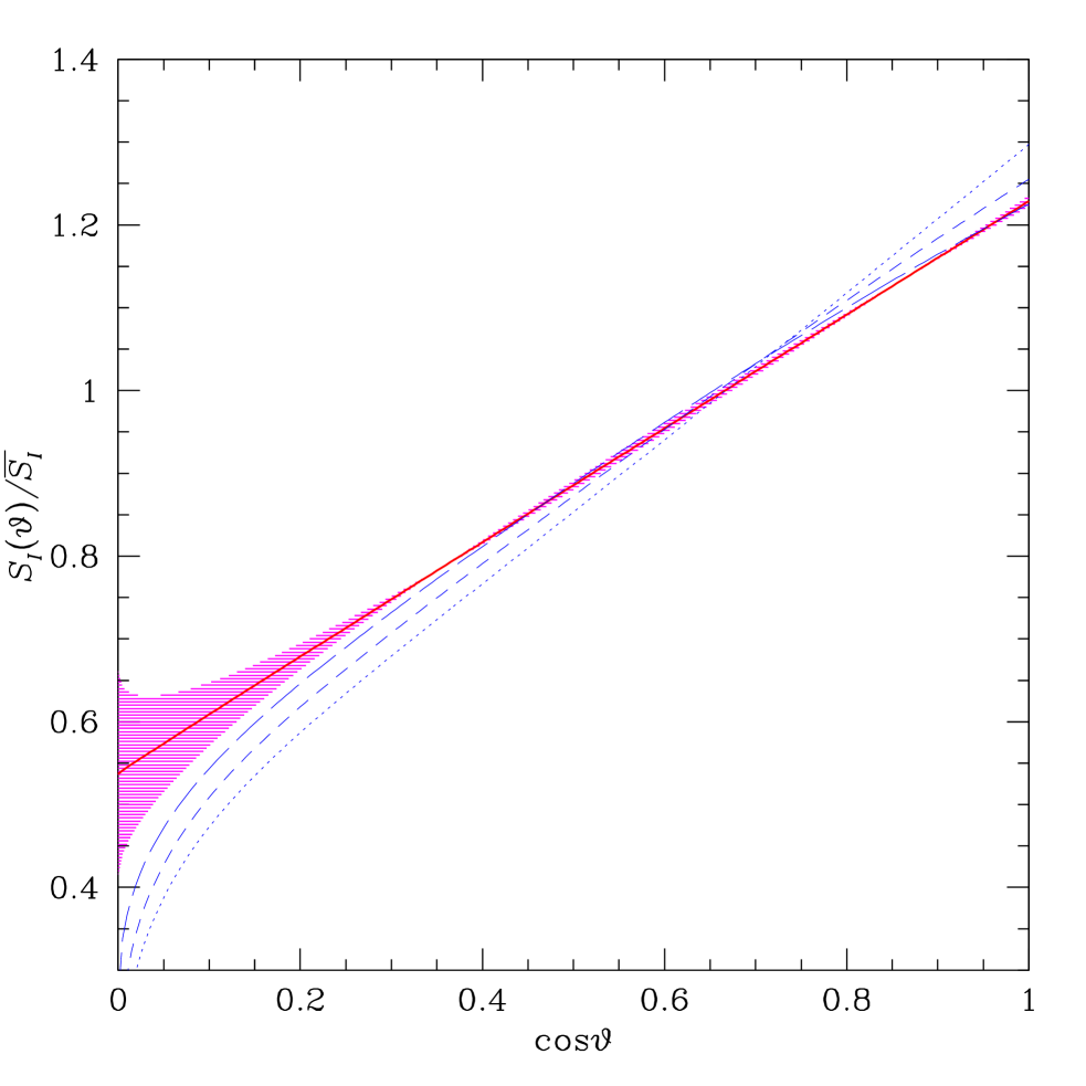
Figure 5: Surface brightness profile of the source star. The thick solid curve is the prediction indicated by the best fit model (see Table 4). In addition, the variation of profiles with the parameters allowed to deviate by 2-$\sigma$ along the direction of the principal conjugate is indicated by a shaded region. For comparison, also shown are theoretical profiles taken from Claret (2000). The stellar atmospheric model parameters for them are $\log g=1.0$, [Fe/H]$=-0.3$, and $T_{\rm eff}=3500\ \mbox{K}$ (dotted curve), $4000\ \mbox{K}$ (short dashed curve), $4500\ \mbox{K}$ (long dashed curve). Note that the effective temperature of the source is reported to be $4500\pm 250\ \mbox{K}$ by Albrow et al. (2001b) and $3800\pm 200\ \mbox{K}$ by Minniti et al. (2002).

Table 3 gives the parameters describing the best-fit microlens model (see Appendix C for details of modeling and Appendix D for the discussion on the error determination) for the PLANET $I$-band observations of EROS BLG-2000-5. We also transform the fit parameters to the set of parameters introduced in § 3.1. In Table 4, we provide the result of limb-darkening coefficient measurements. The measurements of two coefficients, $\Gamma_{I}$ and $\Lambda_{I}$ are highly anti-correlated so that the uncertainty along the major axis of error ellipse is more than 50 times larger than that along its minor axis. While this implies that the constraint on the surface brightness profile derived by the caustic crossing light curve is essentially one dimensional, its natural basis is neither the linear nor the square-root parameterized form. We plot, in Figure 5, the surface brightness profile indicated by the fit and compare these with theoretical calculations taken from Claret (2000). The figure shows that allowing the profile parameters to vary by 2-$\sigma$ does not have much effect on the central slope, but cause a large change in the behavior near the limb. We speculate that this may be related to the specific form of the time sampling over the stellar disk, but more detailed analysis regarding limb darkening is beyond the scope of the present paper and will be discussed elsewhere.

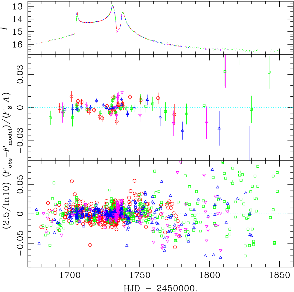
Figure 6: “Magnitude” residuals from PLANET model of EROS BLG-2000-5. Symbols are the same as in Fig. 1 The top panel shows the light curve corresponding to the time of observations, the middle panel shows the averaged residuals from 15-sequential observations, and the bottom panel shows the scatters of individual residual points.

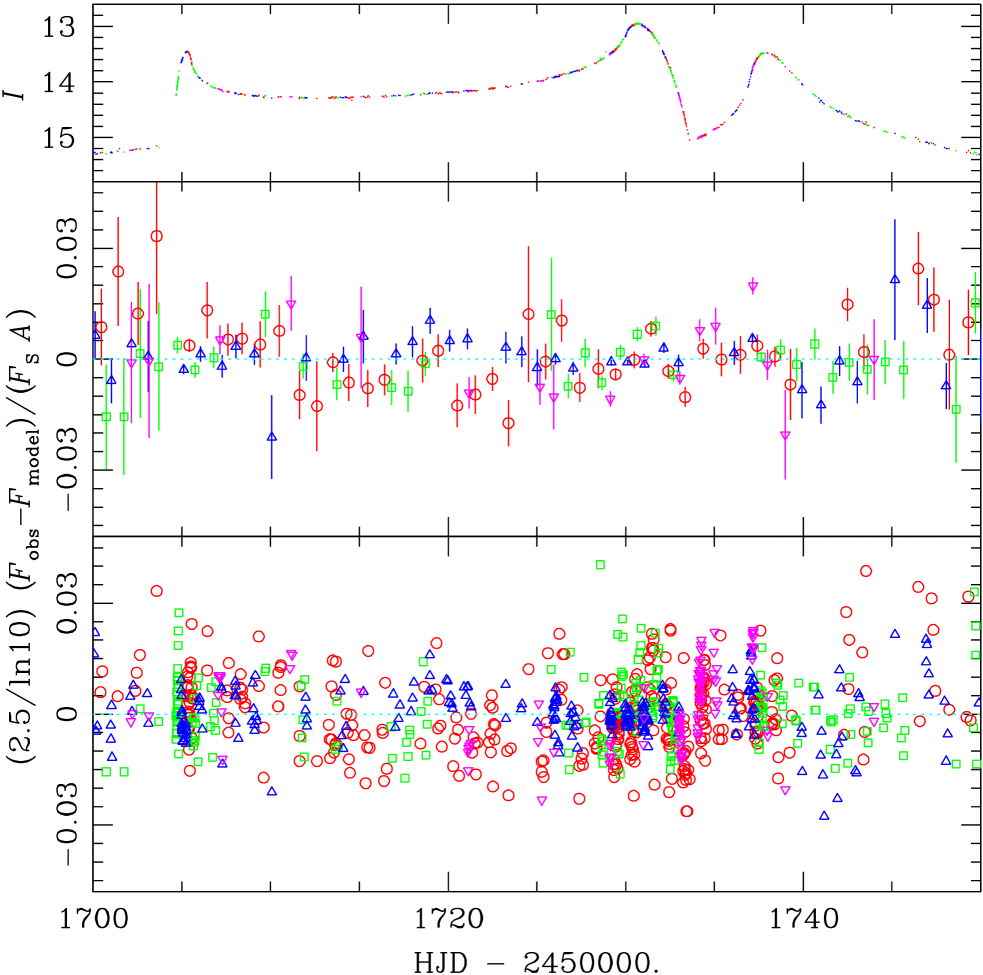
Figure 7: Same as Fig. 6 but focuses mainly on the “anomalous” part of the light curve. The middle panel now shows the daily averages of residuals.

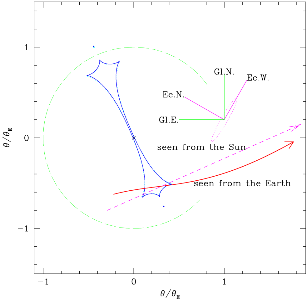
Figure 8: Geometry of the event projected on the sky. Left is Galactic east, up is Galactic north. The origin is the center of mass of the binary lens. The trajectory of the source relative to the lens is shown as a thick solid curve while the short-dashed line shows the relative proper motion of the source seen from the Sun. The lengths of these trajectories correspond to the movement over six months between HJD $=2451670$ and HJD $=2451850$. The circle drawn with long dashes indicates the Einstein ring, and the curves within the circle are the caustics at two different times. The solid curve is at $t=t_{\rm c}$ while the dotted curve is at the time of the first crossing. The corresponding locations of the two lens components are indicated by filled ($t=t_{\rm c}$) and open (the first crossing) dots. The lower dots represent the more massive component of the binary. The ecliptic coordinate basis is also overlayed with the elliptical trajectory of $\pi_{\rm E}\mbox{\boldmath$\varsigma$}$ over the year.

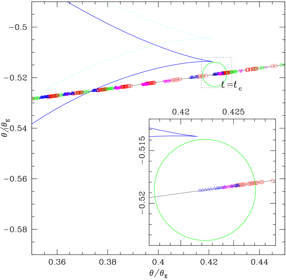
Figure 9: Close-up of Fig. 8 around the cusp approach. The source at the closest approach ($t=t_{\rm c}$) is shown as a circle. The solid curve is the caustic at $t=t_{\rm c}$ while the dotted curve is the caustic at the time of the first crossing. The positions of the source center at the time of each of the observations are also shown by symbols (same as in Figs. 1, 6, 7) that indicate the observatory. For the close-up panel, only those points that were excluded from the fit because of numerical problems in the magnification calculation (see §§ 2 and 4) are shown. Note that the residuals for all points (included these excluded ones) are shown in Figs. 6 and 7.

Figures 6 and 7 show “magnitude residuals”, $(2.5/\ln 10)[\Delta F/(AF_{\rm S})]$, from our best model. Note in particular that the residuals for the points near the cusp approach (HJD $=2451736.944$) that were excluded from the fit do not differ qualitatively from other residuals. It is true that the mean residual for Perth on this night (beginning $4.0\ \mbox{hrs}$ after $t_{\rm c}$ and lasting $2.3\ \mbox{hrs}$) was about 2% high. However, the Canopus data, which span the whole cusp approach from $1.2\ \mbox{hrs}$ before until $7.7\ \mbox{hrs}$ after $t_{\rm c}$, agree with the model to within 0.5%. Moreover, the neighboring SAAO and YALO points also show excellent agreement. See also Fig. 8 and especially Fig. 9.

From the measured microlens parallax ($\pi_{\rm E}=0.277\pm 0.008$), the projected Einstein radius is (eq. [3]);

$$\tilde{r}_{\rm E}=\frac{1\ \mbox{AU}}{\pi_{\rm E}}=3.61\pm 0.11\ \mbox{AU}\ .$$ (12)

We also derive $t_{\rm E}$, the heliocentric Einstein timescale;

$$\mbox{\boldmath$\mu$}_{\rm E}=\dot{\mbox{\boldmath$u$}}_{t_{\rm c}}+\pi_{\rm E}\dot{\mbox{\boldmath$\varsigma$}}_{t_{\rm c}}\,,$$ (13a)

$$t_{\rm E}\equiv|\mbox{\boldmath$\mu$}_{\rm E}|^{-1}=76.8\pm 2.1\ \mbox{days}\,,$$ (13b)

and the direction of $\mbox{\boldmath$\mu$}_{\rm E}$ is $36\fdg 3$ from ecliptic west to south. Since, toward the direction of the event, the Galactic disk runs along 60$\fdg$2 from ecliptic west to south, $\mbox{\boldmath$\mu$}_{\rm E}$ points to $23\fdg 9$ north of the Galactic plane. The overall geometry of the model is shown in Figure 8, and Figure 9 shows a close-up of the geometry in the vicinity of the cusp approach ($t\sim t_{\rm c}$). Next, the projected velocity $\tilde{\mbox{\boldmath$v$}}$ on the observer plane is

$$\tilde{\mbox{\boldmath$v$}}=\tilde{r}_{\rm E}\mbox{\boldmath$\mu$}_{\rm E}=\left(-74.5\pm 3.1,33.0\pm 11.0\right)\ \mbox{km s${}^{-1}$}\ .$$ (14)

Here the vector is expressed in Galactic coordinates. We note that the positive $x$-direction is the direction of the Galactic rotation – i.e. the apparent motion of the Galactic center seen from the Local Standard of Rest (LSR) is in the negative $x$ direction – while the positive $y$-direction is toward the north Galactic pole so that the coordinate basis is left-handed.

5 Measurement of the Angular Einstein Radius

The angular radius of the source, $\theta_{\ast}$, is determined by placing the source on an instrumental CMD and finding its offset relative to the center of the red giant clump, whose de-reddened and calibrated position toward the Galactic bulge are known from the literature. For this purpose, we use the data obtained from YALO. We find the instrumental $I$ magnitude of the (de-blended) source $I_{\rm s}$ from the fit to the light curve. To determine the color, we first note that, except when the source is near (and so partially resolved by) a caustic, microlensing is achromatic. That is, the source is equally magnified in $V$ and $I$: $F_{V}=F_{V,{\rm b}}+AF_{V,{\rm s}}$ and $F_{I}=F_{I,{\rm b}}+AF_{I,{\rm s}}$. Hence, we assemble pairs of $V$ and $I$ points observed within 30 minutes (and excluding all caustic-crossing and cusp-approach data) and fit these to the form $F_{V}=a_{1}+a_{2}F_{I}$. We then find $(V-I)_{\rm s,inst}=-2.5\log a_{2}$. We also find the magnitude of the blend $I_{\rm b}$ from the overall fit, and solve for the color of the blend $(V-I)_{\rm b,inst}=-2.5\log[a_{2}+(a_{1}/F_{I,{\rm b}})]$.

We then locate the source on the instrumental CMD and measure its offset from the center of the red giant clump; $\Delta(V-I)=0.276\pm 0.010$ and $\Delta I=0.33\pm 0.02$. Here, the quoted uncertainty includes terms for both the clump center and the source position. Finally, using the calibrated and de-reddened position of the red clump, $[(V-I)_{0},I_{0}]=[1.114\pm 0.003,14.37\pm 0.02]$ (Paczyński et al., 1999), the source is at $(V-I)_{0}=1.390\pm 0.010$, $I_{0}=14.70\pm 0.03$. The procedure does not assume any specific reddening law for determining the de-reddened source color and magnitude, but may be subject to a systematic error due to differential reddening across the field.

We also perform a photometric calibration for observations made at SAAO. The calibration was derived from images obtained on three different nights by observing Landolt (1992) standards in the 2000 season, and the resulting transformation equation were confirmed with a further night’s observations in 2001. Applying the photometric transformation on the fit result for the source flux, we obtain the – unmagnified – source magnitude of $I=16.602$ in the standard (Johnson/Cousins) system, while the standard source color is measured to be $V-I=2.69$. By adopting the photometric offset between SAAO and YALO instrumental system determined by the fit, we are able to derive a “calibrated” YALO CMD for the field around EROS BLG-2000-5 (Fig. 10). The positions of the source (S), blend (B), and clump center (C) are also overlaid on the CMD. The CMD also implies that the reddening toward the field is $A_{I}=1.90$ and $E(V-I)=1.30$, which yields a reddening law, $R_{VI}=A_{V}/E(V-I)=2.46$, nominally consistent with the generally accepted $R_{VI}=2.49\pm 0.02$ (Stanek, 1996). If we adopt a power-law extinction model $A_{\lambda}\propto\lambda^{-p}$, then $R_{VI}=2.46$ corresponds to $p=1.37$. For this index, $E(\bv)/E(V-I)=0.838$, which predicts a lower extinction than the spectroscopically determined reddening of $E(\bv)=1.30\pm 0.05$ by Albrow et al. (2001b).

Both the source and the blend lie redward of the main population of stars in the CMD. One possible explanation is that the line of sight to the source is more heavily reddened than average due to differential reddening across the field. Inspection of the images does indicate significant differential reddening, although from the CMD itself it is clear that only a small minority of stars in the field could suffer the additional $\Delta A_{V}\sim 0.7$ that would be necessary to bring the source to the center of the clump. There is yet another indication that the source has average extinction for the field – i.e. the same or similar extinction as the clump center. The de-reddened (intrinsic) color derived on this assumption, $(V-I)_{0}=1.39$ is typical of a K3III star (Bessell & Brett, 1988), which is in good agreement with the spectral type determined by Albrow et al. (2001b). On the other hand, if the source were a reddened clump giant with $(V-I)_{0}\sim 1.11$, then it should be a K1 or K2 star.

We then apply the procedure of Albrow et al. (2000a) to derive the angular source radius $\theta_{\ast}$ from its de-reddened color and magnitude: first we use the color-color relations of Bessell & Brett (1988) to convert from $(V-I)_{0}$ to $(V-K)_{0}$, and then we use the empirical relation between color and surface brightness to obtain $\theta_{\ast}$ (van Belle, 1999). From this, we find that

$$\theta_{\ast} = 6.62\pm 0.58\ \mbox{$\mu$as}$$ (15)

$$= 1.42\pm 0.12\ \mbox{R${}_{\sun}$ kpc${}^{-1}$}\,,$$

where the error is dominated by the 8.7% intrinsic scatter in the relation of van Belle (1999). Alternatively, we use the different calibration derived for K giants by Beuermann, Baraffe, & Hauschildt (1999) and obtain $\theta_{\ast}=6.47\ \mbox{$\mu$as}$, which is consistent with equation (15). Finally, we note that if the source were actually a clump giant that suffered $\Delta A_{V}=0.7$ extra extinction, its angular size would be $7.08\ \mbox{$\mu$as}$. Since we consider this scenario unlikely, and since in any event the shift is smaller than the statistical error, we ignore this possibility.

From this determination of $\theta_{\ast}$ and the value, $\rho_{\ast}=(4.80\pm 0.04)\times 10^{-3}$, determined from the fit to the light curve, we finally obtain,

$$\theta_{\rm E}=\frac{\theta_{\ast}}{\rho_{\ast}}=1.38\pm 0.12\ \mbox{mas}\,,$$ (16)

where the error is again dominated by the intrinsic scatter in the relation of van Belle (1999).

6 The Lens Mass and the Lens-Source Relative Proper Motion

By combining the results obtained in §§ 4 and 5, one can derive several key physical parameters, including the lens mass and the lens-source relative parallax and proper motion;

$$M=\frac{c^{2}}{4G}\tilde{r}_{\rm E}\theta_{\rm E}=0.612\pm 0.057\ \mbox{M}_{\sun}\,,$$ (17)

$$D_{\rm rel}=\frac{\tilde{r}_{\rm E}}{\theta_{\rm E}}=2.62\pm 0.24\ \mbox{kpc}\,;$$ (18a)

$$\pi_{\rm L}-\pi_{\rm S}=\frac{\mbox{1 AU}}{D_{\rm rel}}=0.382\pm 0.035\ \mbox{mas}\ .$$ (18b)

$$|\mbox{\boldmath$\mu$}_{\rm S}-\mbox{\boldmath$\mu$}_{\rm L}|=\theta_{\rm E}|\mbox{\boldmath$\mu$}_{\rm E}| = 18.0\pm 1.7\ \mbox{$\mu$as day${}^{-1}$}$$ (19)

$$= 31.1\pm 2.9\ \mbox{km s${}^{-1}$ kpc${}^{-1}$}\ .$$

For the binary mass ratio of the best-fit model, $q=0.749$, the masses of the individual components are $0.350\ \mbox{M${}_{\sun}$}$ and $0.262\ \mbox{M${}_{\sun}$}$, both of which are consistent with the mass of typical mid-M dwarfs in the Galactic disk. Using the mass-luminosity relation of Henry & McCarthy (1993), and adopting $M_{V}=2.89+3.37(V-I)$, the binary then has a combined color and magnitude $M_{I}=8.2\pm 0.2$ and $(V-I)=2.54\pm 0.08$. Since $D_{\rm rel}^{-1}=D_{\rm L}^{-1}-D_{\rm S}^{-1}$, $D_{\rm rel}$ is an upper limit for $D_{\rm L}$, i.e. the lens is located in the Galactic disk within $2.6\ \mbox{kpc}$ of the Sun. Furthermore, an argument based on the kinematics (see § 7) suggests that $D_{\rm S}\gtrsim 8\ \mbox{kpc}$ so that it is reasonable to conclude that $D_{\rm L}\sim 2\ \mbox{kpc}$ ($m-M\simeq 11.5$). Hence, even if the binary lens lay in front of all the extinction along the line of sight, it would be $\sim 2\ \mbox{mag}$ fainter than the blend (B), and so cannot contribute significantly to the blended light. However, the proximity of the lens to the observer is responsible for the event’s long time scale and quite large parallax effect.

7 The Kinematic Constraints on the Source Distance

The projected velocity $\tilde{\mbox{\boldmath$v$}}$ (eq. [14]) is related to the kinematic parameters of the event by

$$\tilde{\mbox{\boldmath$v$}} = D_{\rm rel}\left(\mbox{\boldmath$\mu$}_{\rm S}-\mbox{\boldmath$\mu$}_{\rm L}\right)$$ (20a)

$$= \left(D_{\rm rel}\frac{\mbox{\boldmath$v$}_{\rm S}}{D_{\rm S}}-D_{\rm rel}\frac{\mbox{\boldmath$v$}_{\rm L}}{D_{\rm L}}+\mbox{\boldmath$v$}_{\sun}\right)_{\perp}\,,$$

where the final subscript, $$\perp \mbox{\boldmath$v$}_{\sun}=\mbox{\boldmath$v$}_{\rm rot}+\mbox{\boldmath$v$}_{\sun,{\rm p}} \mbox{\boldmath$v$}_{\rm L}=\mbox{\boldmath$v$}_{\rm rot}+\mbox{\boldmath$v$}_{\rm L,p} D_{\rm L} D_{\rm rel} D_{\rm S}$$, serves to remind us that all velocities are projected onto the plane of the sky. Writing and as the sum of the Galactic rotation and the peculiar velocities and eliminating in favor of and , equation (20a) can be expressed as

$$\tilde{\mbox{\boldmath$v$}}=\left[\frac{D_{\rm rel}}{D_{\rm S}}(\mbox{\boldmath$v$}_{\rm S}-\mbox{\boldmath$v$}_{\rm rot})-\left(1+\frac{D_{\rm rel}}{D_{\rm S}}\right)\mbox{\boldmath$v$}_{\rm L,p}+\mbox{\boldmath$v$}_{\sun,{\rm p}}\right]_{\perp}\ .$$ (20b)

For a fixed $D_{\rm S}$ and with a known Galactic kinematic model, the distribution function of the expected value for $\tilde{\mbox{\boldmath$v$}}$ can be derived from equation (20b). The measured value of $\tilde{\mbox{\boldmath$v$}}$ can therefore be translated into the relative likelihood, ${\mathcal{L}}$ for a given $D_{\rm S}$ and the assumed kinematic model,

$$-2\ln{\mathcal{L}}=(\tilde{\mbox{\boldmath$v$}}-\langle\tilde{\mbox{\boldmath$v$}}\rangle)\cdot\mathbf{C}^{-1}\cdot(\tilde{\mbox{\boldmath$v$}}-\langle\tilde{\mbox{\boldmath$v$}}\rangle)+\ln|\mathbf{C}|+{\rm constant}\,,$$ (21a)

$$\langle\tilde{\mbox{\boldmath$v$}}\rangle=x_{\rm S}(\langle\mbox{\boldmath$v$}_{{\rm S},\perp}\rangle-\mbox{\boldmath$v$}_{\rm rot})-(1+x_{\rm S})\langle\mbox{\boldmath$v$}_{{\rm L,p},\perp}\rangle+\mbox{\boldmath$v$}_{\sun,{\rm p},\perp}\,,$$ (21b)

$$\mathbf{C}=x_{\rm S}^{2}\mathbf{C}[\mbox{\boldmath$v$}_{{\rm S},\perp}]+(1+x_{\rm S})^{2}\mathbf{C}[\mbox{\boldmath$v$}_{{\rm L},\perp}]+\mathbf{C}[\tilde{\mbox{\boldmath$v$}}]\,,$$ (21c)

where $\mathbf{C}[\mbox{\boldmath$v$}_{{\rm S},\perp}]$ and $\mathbf{C}[\mbox{\boldmath$v$}_{{\rm L},\perp}]$ are the dispersion tensors for the source and the lens transverse velocity, $\mathbf{C}[\tilde{\mbox{\boldmath$v$}}]$ is the covariance tensor for the measurement of $\tilde{\mbox{\boldmath$v$}}$, and $x_{\rm S}=D_{\rm rel}/D_{\rm S}$.

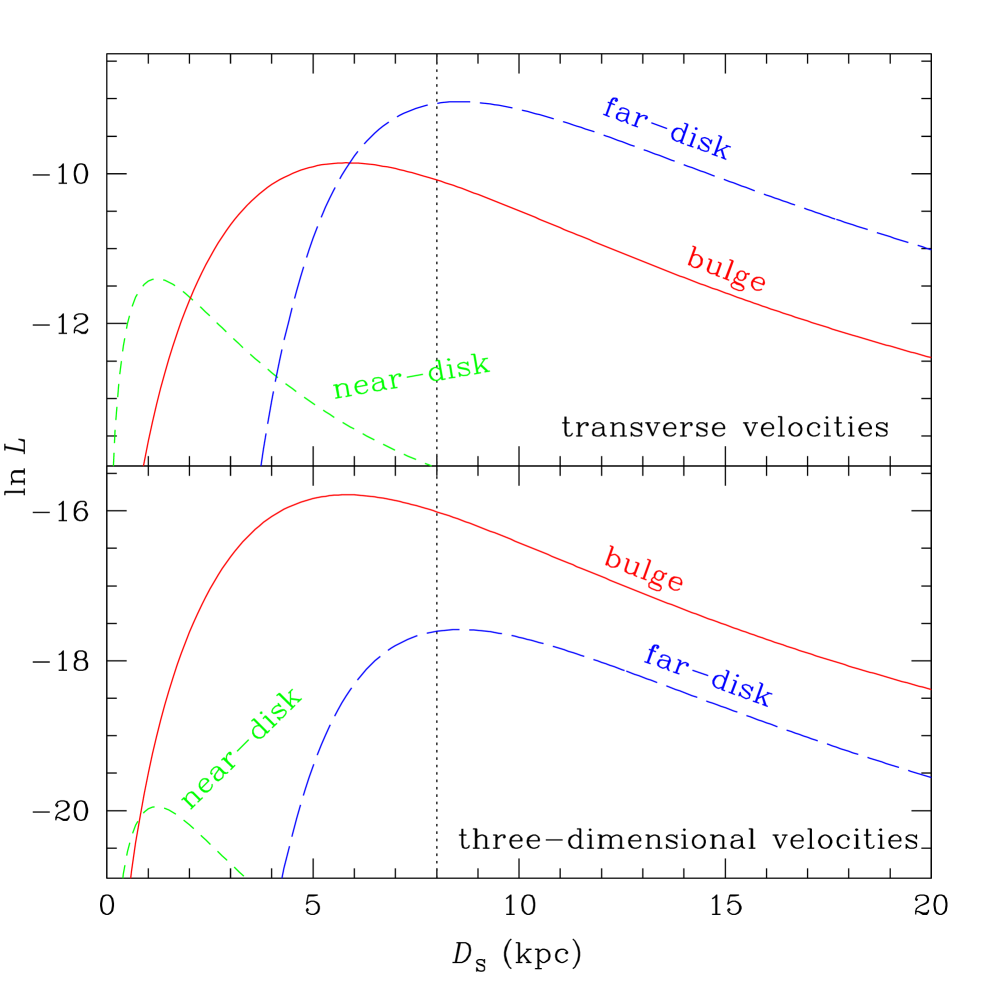
Figure 11: Kinematic likelihood for $\tilde{\mbox{\boldmath$v$}}$ as a function of $D_{\rm S}$. The three curves are for different distributions of the source velocity: near-disk-like; $\mbox{\boldmath$v$}_{\rm S}=\mbox{\boldmath$v$}_{\rm rot}+\mbox{\boldmath$v$}_{\rm S,p}$ (short-dashed line), bulge-like; $\mbox{\boldmath$v$}_{\rm S}=\mbox{\boldmath$v$}_{\rm S,p}$ (solid line), and far-disk-like; $\mbox{\boldmath$v$}_{\rm S}=-\mbox{\boldmath$v$}_{\rm rot}-\mbox{\boldmath$v$}_{\rm S,p}$ (long-dashed line). The top panel shows the likelihood derived using only the two-dimensional projected velocity information while in the bottom panel, the likelihood also includes the radial velocity information derived from the high resolution spectra of Castro et al. (2001).

We evaluate ${\mathcal{L}}$ as a function of $D_{\rm S}$ assuming three different distributions for $\mbox{\boldmath$v$}_{{\rm S},\perp}$ which respectively correspond to source being in the near disk ($\langle\mbox{\boldmath$v$}_{{\rm S},\perp}\rangle=\mbox{\boldmath$v$}_{\rm rot}+\langle\mbox{\boldmath$v$}_{{\rm S,p},\perp}\rangle$), bulge ($\langle\mbox{\boldmath$v$}_{{\rm S},\perp}\rangle=\langle\mbox{\boldmath$v$}_{{\rm S,p},\perp}\rangle$), and the far disk ($\langle\mbox{\boldmath$v$}_{{\rm S},\perp}\rangle=-\mbox{\boldmath$v$}_{\rm rot}-\langle\mbox{\boldmath$v$}_{{\rm S,p},\perp}\rangle$). Adopting the Galactic rotational velocity, $\mbox{\boldmath$v$}_{\rm rot}=(220,0)\ \mbox{km s${}^{-1}$}$, the solar motion, $\mbox{\boldmath$v$}_{\sun,{\rm p},\perp}=(5.2,7.2)\ \mbox{km s${}^{-1}$}$ (Binney & Merrifield, 1998), and the kinematic characteristics of the lens and the source given in Table 5, we derive the relative likelihood as a function of source position (Fig. 11), and find that the measured value of $\tilde{\mbox{\boldmath$v$}}$ (eq. [14]) mildly favors the far disk over the bulge as the location of the source by a factor of $\sim 2.3$. The near disk location is quite strongly disfavored (by a factor of $\sim 10.6$ compared to the far disk, and by a factor of $\sim 4.7$ compared to the bulge).

The complete representation of the likelihood for the source location requires one to consider all the available constraints relevant to the source distance. In particular, these include the radial (line-of-sight) velocity measurement and the number density of stars constrained by the measured color and brightness (or luminosity) along the line of sight. Although one may naively expect that a bulge location is favored by the high density of stars in the bulge, which follows from the fact that the line of sight passes within 400 pc of the Galactic center, it is not immediately obvious how the disk contribution compares to the bulge stars for the specific location of the source on the CMD (Fig. 10). Even with no significant differential reddening over the field, the particular source position, which is both fainter and redder than the center of the clump, can be occupied by relatively metal-rich (compared to the bulge average) first ascent giants in either the bulge or the far disk. Because first ascent giants become redder with increasing luminosity, the source must have higher metallicity if it lies in the bulge than in the more distant disk. There exist two estimate of the source metal abundance: [Fe/H]$=-0.3\pm 0.1$ by Albrow et al. (2001b) based on VLT FORS1 spectra and [Fe/H]$=-0.3\pm 0.3$ by Minniti et al. (2002) based on VLT UVES spectra. However, to incorporate these measurement into a likelihood estimate would require a more through understanding of all the sources of error as well as a detailed model of the metallicity distribution of the bulge and the disk. For this reason, we defer the proper calculation of the likelihood in the absence of any definitive way to incorporate the specific density function, and restrict ourselves to the kinematic likelihood.

We determine the radial velocity of the source from Keck HIRES spectra of Castro et al. (2001), kindly provided to us by R. M. Rich. We find the line-of-sight velocity to be $\sim-100\ \mbox{km s${}^{-1}$}$ (blueshift; heliocentric), which translates to $\sim-90\ \mbox{km s${}^{-1}$}$ Galactocentric radial velocity accounting for the solar motion of $10\ \mbox{km s${}^{-1}$}$. The derived radial velocity strongly favors bulge membership of the source since it is three times larger than the line-of-sight velocity dispersion for disk K3 giants, but is consistent with the motions of typical bulge stars (c.f. Table 5). Because the correlation between the radial and the transverse velocity for K3 giants either in the disk or in the bulge is very small, the likelihood for the radial velocity can be estimated independently from the likelihood for the transverse velocity, and the final kinematic likelihood is a simple product of two components. We find that the final kinematic likelihood including the radial velocity information indicates that the source star belongs to the bulge (Fig. 11): the likelihood for the bulge membership is about six times larger than that for the far disk membership.

Finally, we note that, if the source lay in the far disk, it should have an additional retrograde proper motion of $\sim 4\ \mbox{mas yr${}^{-1}$}\times(10\ \mbox{kpc}/D_{\rm S})$ with respect to the bulge stars, which should be measurable using adaptive optics or the Hubble Space Telescope.

8 Consistency between the Lens Mass and the Binary Orbital Motion

For the derived parameters, we find a projected binary lens separation $r_{\perp}=d\,D_{\rm L}\theta_{\rm E}=5.52\ \mbox{AU}$ $(5.25\ \mbox{AU})$ and transverse orbital speed $v_{\perp}=[\dot{d}^{2}+(\omega d)^{2}]^{1/2}D_{\rm L}\theta_{\rm E}=2.76\ \mbox{km s${}^{-1}$}$ $(2.62\ \mbox{km s${}^{-1}$})$ for $D_{\rm S}=10\ \mbox{kpc}$ $(8\ \mbox{kpc})$. We can now define the transverse kinetic and potential energies $K_{\perp}=[q/(1+q)^{2}]Mv_{\perp}^{2}/2$ and $T_{\perp}=-[q/(1+q)^{2}]GM^{2}/r_{\perp}$, and evaluate their ratio,

$$\varrho=\left|\frac{T_{\perp}}{K_{\perp}}\right|=\frac{2GM}{r_{\perp}v_{\perp}^{2}}=\frac{c^{2}}{2}\frac{\tilde{r}_{\rm E}\theta_{\rm E}[\tilde{r}_{\rm E}^{-1}+(D_{\rm S}\theta_{\rm E})^{-1}]^{3}}{d[{\dot{d}}^{2}+(\omega d)^{2}]}=25.9\pm 5.1\ \ (D_{\rm S}=10\ \mbox{kpc})\ .$$ (22)

Here, the error is dominated by the uncertainty in the measurement of $\omega$. Since $r_{\perp}\leq r$ and $v_{\perp}\leq v$, it follows that $|T_{\perp}|\geq|T|$ and $K_{\perp}\leq K$, and hence $|T_{\perp}/K_{\perp}|\geq|T/K|$, where $|T/K|$ is the ratio of the true three-dimensional potential and kinetic energies. The latter must be greater than unity for a gravitationally bound binary. This constraint is certainly satisfied by EROS BLG-2000-5. Indeed, perhaps it is satisfied too well. That is, what is the probability of detecting such a large ratio of projected energies? To address this question, we numerically integrate over binary orbital parameters (viewing angles, the orbital orientation and phase, and the semi-major axis) subject to the constraint that $r_{\perp}=5.5\ \mbox{AU}$ ($D_{\rm S}=10\ \mbox{kpc}$), and at several fixed values of the eccentricity, $e$. We assume a random ensemble of viewing angles and orbital phases. The results shown in Figure 12 assume a Duquennoy & Mayor (1991) period distribution, but are almost exactly the same if we adopt a flat period distribution. All of the eccentricities shown in Figure 12 are reasonably consistent with the observed ratio, although higher eccentricities are favored.

One can also show that high eccentricities are favored using another line of argument. First, note that $|\mbox{\boldmath$r$}_{\perp}\times\mbox{\boldmath$v$}_{\perp}|=\omega r_{\perp}^{2}$ is the same as the projection of the specific angular momentum of the binary to the line of sight, $|(\mbox{\boldmath$r$}\times\mbox{\boldmath$v$})\cdot\hat{\mbox{\boldmath$n$}}|=2\pi a^{2}(1-e^{2})|\cos i|/P$. Here $a$ and $P$ are the semi-major axis and the orbital period of the binary, $\hat{\mbox{\boldmath$n$}}$ is the line-of-sight unit vector, and $i$ is the inclination angle of the binary. Combining this result with Kepler’s Third Law, $4\pi^{2}a^{3}=GMP^{2}$, one obtains (here and throughout this section, we assume that $D_{\rm S}=10\ \mbox{kpc}$);

$$a(1-e^{2})^{2}\cos^{2}i=\frac{(\omega r_{\perp}^{2})^{2}}{GM}=\frac{4}{c^{2}}\frac{\omega^{2}d^{4}}{\tilde{r}_{\rm E}\theta_{\rm E}[\tilde{r}_{\rm E}^{-1}+(D_{\rm S}\theta_{\rm E})^{-1}]^{4}}=0.0013\pm 0.0341\ \mbox{AU}\ .$$ (23)

From the energy conservation, $(v^{2}/2)-(GM/r)=-GM/(2a)$, one may derive a lower limit for $a$;

$$a=\frac{r}{2}\left(1-\frac{rv^{2}}{2GM}\right)^{-1}\geq\frac{r_{\perp}}{2(1-\varrho^{-1})}=2.87\pm 0.09\ \mbox{AU}\ .$$ (24)

The corresponding lower limit for the binary period is $P\geq 6.22\ \mbox{yr}$ for $D_{\rm S}=10\ \mbox{kpc}$. Now, we can derive a constraint on the allowed eccentricity and inclination by dividing equation (23) by equation (24);

$$(1-e^{2})|\cos i|\leq 0.021\pm 0.281\ .$$ (25)

The constraint here essentially arises from the fact that the fit barely detects projected angular motion $\omega$, while the formal precision of its measurement corresponds to $\sim 80\ \mbox{yr}$ orbital period in 1-$\sigma$ level. For the observed projected separation and the derived binary mass, this apparent lack of the binary angular motion therefore naturally leads us to conclude that the binary orbit is either very close to edge-on or highly eccentric (or both).

9 Another Look at MACHO 97-BLG-41

We have found that both parallax and binary orbital motion are required to explain the deviations from rectilinear motion exhibited by the light curve of EROS BLG-2000-5. In a previous paper about another event, MACHO 97-BLG-41 (Albrow et al., 2000a), we had ascribed all deviations from rectilinear motion to a single cause: projected binary orbital motion. Could both effects have also been significant in that event as well? Only detailed modeling can give a full answer to this question. However, we can give a rough estimate of the size of the projected Einstein ring $\tilde{r}_{\rm E}$ that would be required to explain the departures from linear motion seen in that event.

Basically what we found in the case of MACHO 97-BLG-41 was that the light curve in the neighborhood of the central caustic (near HJD $\sim 2450654$) fixed the lens geometry at that time, and so predicted both the position of the outlying caustics and the instantaneous velocity of the source relative to the Einstein ring. If this instantaneous relative velocity were maintained, then the source would have missed this outlying caustic by about $\Delta u_{\rm obs}\sim 0.4$ (Albrow et al., 2000a, fig. 3). On the other hand, the predicted displacement of a caustic due to parallax is

$$\Delta\mbox{\boldmath$u$}_{\rm pred}=-\pi_{\rm E}\mbox{\boldmath$\mathcal{D}$}_{\rm P}\,;$$ (26a)

$$\mbox{\boldmath$\mathcal{D}$}_{\rm P}=\mbox{\boldmath$\varsigma$}_{t_{{\rm cc},1}}-\mbox{\boldmath$\varsigma$}_{t_{{\rm cc},2}}-(t_{{\rm cc},1}-t_{{\rm cc},2})\dot{\mbox{\boldmath$\varsigma$}}_{t_{{\rm cc},2}}\ .$$ (26b)

We find $|\mbox{\boldmath$\mathcal{D}$}_{\rm P}|=0.072$, and hence,

$$\pi_{\rm E}=5.6\ \frac{\Delta u_{\rm pred}}{\Delta u_{\rm obs}}\ .$$ (27)

That is, to explain by parallax the order of the effect seen requires $\tilde{r}_{\rm E}\sim 0.18\ \mbox{AU}$, which (using the measured $\theta_{\rm E}=0.7\ \mbox{mas}$) would in turn imply a lens mass $M\sim 0.015\ \mbox{M${}_{\sun}$}$, a lens distance of $D_{\rm L}\lesssim 250\ \mbox{pc}$, and the projected lens-source relative transverse velocity on the observer plane (at time $t_{\rm cc,2}$) of only $13\ \mbox{km s${}^{-1}$}$. While these values cannot be strictly ruled out, they are a priori extremely unlikely because the optical depth to such nearby, low-mass, and slow lenses is extremely small. On the other hand, if the lens lies at a distance typical of bulge lenses $D_{\rm L}\sim 6\ \mbox{kpc}$ and the source is a bulge star, then $\tilde{r}_{\rm E}=D_{\rm rel}\theta_{\rm E}\sim 17\ \mbox{AU}$, which would imply $\Delta u_{\rm pred}/\Delta u_{\rm obs}\sim 1\%$. That is, parallax would contribute negligibly to the observed effect. We therefore conclude that most likely parallax does not play a major role in the interpretation of MACHO 97-BLG-41, but that detailed modeling will be required to determine to what extent such a role is possible.

What is the physical reason that parallax must be so much stronger (i.e., $\pi_{\rm E}$ must be so much bigger) to have a significant effect in the case of MACHO 97-BLG-41 than for EROS BLG-2000-5? Fundamentally, the former is a close binary, and there is consequently a huge “lever arm” between the radial position of the outlying caustic, $u_{\rm c}\sim 1.7$ and the binary separation, $d\sim 0.5$. That is $u_{\rm c}/d\sim 3.2$. This is almost an order of magnitude larger than for EROS BLG-2000-5, for which $u_{\rm c}\sim 0.8$ (Fig. 8), $d\sim 1.9$, and $u_{\rm c}/d\sim 0.4$. Consequently, parallax has to be an order of magnitude larger to reproduce the effects of the same amount of the projected binary orbital motion.

10 Summary

We have presented here results from two seasons of photometric $I$-band monitoring of the microlensing event EROS BLG-2000-5, made by the PLANET collaboration. The light curve exhibits two peaks which are well explained by a finite source crossing over a fold-type – inverse-square-root singularity – caustic, followed by a third peak which is due to the source’s passage close to a cusp. We find no geometry involving a rectilinear source-lens relative trajectory and a static lens that is consistent with the photometry. However, by incorporating both parallax and binary orbital motion, we are able to model the observed light curve. In particular, the detection of the parallax effect is important because it enables us to derive the microlens mass, $M=0.612\pm 0.057\ \mbox{M}_{\sun}$, unambiguously by the combination of the projected Einstein radius – measured from the parallax effect – and the angular Einstein radius – inferred from the source angular size and the finite source effect on the light curve. The source size is measurable from the magnitude and the color of the source. The kinematic properties of the lens/source system derived from our model together with the lens-source relative parallax measurement as well as an additional radial velocity measurement indicate that the event is most likely caused by a (K3) giant star in the bulge being lensed by a disk binary (M dwarf) system about $2\ \mbox{kpc}$ from the Sun. Additional information on the specific density function along the line of sights, differential reddening across the field, and a metallicity measurement of the source could further constrain the source location.

Appendix A Determination of $\varsigma$

If $s$ is the Sun’s position vector with respect to the Earth normalized by $1\ \mbox{AU}$, then the projection of $s$ onto the plane of the sky, $\varsigma$, is

$$\mbox{\boldmath$\varsigma$}=\mbox{\boldmath$s$}-(\mbox{\boldmath$s$}\cdot\hat{\mbox{\boldmath$n$}})\hat{\mbox{\boldmath$n$}}\,,$$ (A1)

where $\hat{\mbox{\boldmath$n$}}$ is the line-of-sight unit vector toward the position of the event on the sky, while the projection of $\hat{\mbox{\boldmath$p$}}$, the unit vector toward the north ecliptic pole (NEP), is given by $\tilde{\mbox{\boldmath$p$}}=\hat{\mbox{\boldmath$p$}}-(\hat{\mbox{\boldmath$p$}}\cdot\hat{\mbox{\boldmath$n$}})\hat{\mbox{\boldmath$n$}}$. Then, ($\varsigma_{w},\varsigma_{n}$), the ecliptic coordinate components of $\varsigma$, are

$$\varsigma_{w}=\frac{(\tilde{\mbox{\boldmath$p$}}\times\mbox{\boldmath$\varsigma$})\cdot\hat{\mbox{\boldmath$n$}}}{|\tilde{\mbox{\boldmath$p$}}|}=\frac{(\hat{\mbox{\boldmath$p$}}\times\mbox{\boldmath$s$})\cdot\hat{\mbox{\boldmath$n$}}}{\sqrt{1-(\hat{\mbox{\boldmath$p$}}\cdot\hat{\mbox{\boldmath$n$}})^{2}}}\,,$$ (A2a)

$$\varsigma_{n}=\frac{\tilde{\mbox{\boldmath$p$}}\cdot\mbox{\boldmath$\varsigma$}}{|\tilde{\mbox{\boldmath$p$}}|}=-\frac{(\hat{\mbox{\boldmath$p$}}\cdot\hat{\mbox{\boldmath$n$}})(\mbox{\boldmath$s$}\cdot\hat{\mbox{\boldmath$n$}})}{\sqrt{1-(\hat{\mbox{\boldmath$p$}}\cdot\hat{\mbox{\boldmath$n$}})^{2}}}\,,$$ (A2b)

where we make use of $\hat{\mbox{\boldmath$p$}}\cdot\mbox{\boldmath$s$}=0$. One can choose three-dimensional coordinate axes so that the $x$-axis is the direction of the vernal equinox, the $z$-axis is the direction to the NEP, and $\hat{\mbox{\boldmath$y$}}=\hat{\mbox{\boldmath$z$}}\times\hat{\mbox{\boldmath$x$}}$. Then,

$$\hat{\mbox{\boldmath$p$}}=(0,0,1)\,;$$ (A3a)

$$\mbox{\boldmath$s$}=(r_{\earth}\cos\lambda_{\sun},r_{\earth}\sin\lambda_{\sun},0)\,;$$ (A3b)

$$\hat{\mbox{\boldmath$n$}}=(\cos\lambda_{0}\cos\beta_{0},\sin\lambda_{0}\cos\beta_{0},\sin\beta_{0})\,,$$ (A3c)

where $r_{\earth}$ is the distance to the Sun from the Earth in units of AU, $\lambda_{\sun}$ is the Sun’s ecliptic longitude, and ($\lambda_{0},\beta_{0}$) are the ecliptic coordinates of the event. By substituting equations (A3) into equations (A2), one finds that

$$\varsigma_{w}=-r_{\earth}\sin(\lambda_{\sun}-\lambda_{0})\,,$$ (A4a)

$$\varsigma_{n}=-r_{\earth}\cos(\lambda_{\sun}-\lambda_{0})\sin\beta_{0}\ .$$ (A4b)

In general, one must consider the Earth’s orbital eccentricity ($\epsilon=1.67\times 10^{-2}$) to calculate $\varsigma$ for any given time. Then,

$$r_{\earth}=1-\epsilon\cos\psi\,;\ \ \ \lambda_{\sun}=\xi-\phi_{\Upsilon}\,,$$ (A5a)

$$\psi-\epsilon\sin\psi=\Omega t\,,$$ (A5b)

$$\sin\xi=\frac{(1-\epsilon^{2})^{1/2}\sin\psi}{1-\epsilon\cos\psi}\,;\ \ \ \cos\xi=\frac{\cos\psi-\epsilon}{1-\epsilon\cos\psi}\,,$$ (A5c)

where $\psi$ and $\xi$ are the eccentric and true anomalies of the Earth, $\phi_{\Upsilon}=77\fdg 86$ is the true anomaly at the vernal equinox (March 20, 07^h35^m UT for 2000; Larsen & Holdaway, 1999), $t$ is the time elapsed since perihelion, and $\Omega=2\pi\ \mbox{yr${}^{-1}$}$. Note that the Earth was at perihelion at January 3, 05^h UT for 2000 (Larsen & Holdaway, 1999). Although equations (A5) cannot be solved for $r_{\earth}$ and $\lambda_{\sun}$ in closed form as functions of $t$, one can expand in series with respect to $\epsilon$ and approximate up to the first order (epicycle approximation) so that

$$r_{\earth}=1-\epsilon\cos(\Omega t)\,;\ \ \ \lambda_{\sun}=\Omega t-\phi_{\Upsilon}+2\epsilon\sin(\Omega t)\ .$$ (A6)

Appendix B Microlens Diurnal Parallax

The angular position of a celestial object observed from an observatory on the surface of the Earth is related to its geocentric angular position, $\mbox{\boldmath$\varphi$}_{\rm X}$ by

$$\mbox{\boldmath$\varphi$}^{\prime}_{\rm X}=\mbox{\boldmath$\varphi$}_{\rm X}-\frac{\mbox{\boldmath$\gamma$}\mbox{R}_{\earth}}{D_{\rm X}}\,,$$ (B1)

where

$$\mbox{\boldmath$\gamma$}=\mbox{\boldmath$r$}-(\mbox{\boldmath$r$}\cdot\hat{\mbox{\boldmath$n$}})\hat{\mbox{\boldmath$n$}}$$ (B2)

is the projection of the position vector, $r$, of the observatory with respect to the center of the Earth, onto the plane of the sky and normalized by the mean radius of the Earth, R_⊕; and $D_{\rm X}$ and $\hat{\mbox{\boldmath$n$}}$ are the distance and the line-of-sight vector to the object of interest. If one observe a microlensing event, the actual dimensionless lens-source separation vector therefore differs from $u$ (eq. [6]) by

$$\mbox{\boldmath$u$}^{\prime} = \frac{\mbox{\boldmath$\varphi$}^{\prime}_{\rm S}-\mbox{\boldmath$\varphi$}^{\prime}_{\rm L}}{\theta_{\rm E}}=\mbox{\boldmath$u$}+\frac{\mbox{R}_{\earth}}{\tilde{r}_{\rm E}}\mbox{\boldmath$\gamma$}$$ (B3)

$$= \mbox{\boldmath$\upsilon$}+(t-t_{\rm c})\mbox{\boldmath$\mu$}_{\rm E}-\pi_{\rm E}(\mbox{\boldmath$\varsigma$}-\frac{\mbox{R}_{\earth}}{1\ \mbox{AU}}\mbox{\boldmath$\gamma$})\ .$$

To find the algebraic expression for ecliptic coordinate components of $\gamma$, we choose the same coordinate axes as for equations (A3). Then, the position vector, $r$ is expressed as

$$\mbox{\boldmath$r$}=(\cos\delta_{\rm g}\cos\tau_{\Upsilon},\cos\delta_{\rm g}\sin\tau_{\Upsilon}\cos\varepsilon+\sin\delta_{\rm g}\sin\varepsilon,\sin\delta_{\rm g}\cos\varepsilon-\cos\delta_{\rm g}\sin\tau_{\Upsilon}\sin\varepsilon)\,,$$ (B4)

where $\delta_{\rm g}$ is the geographic latitude of the observatory, $\tau_{\Upsilon}$ is the hour angle of the vernal equinox (i.e. the angle of the local sidereal time) at the observation, and $\varepsilon=23\fdg 44$ is the angle between the direction toward the north celestial pole and the NEP (here we also assume that the Earth is a perfect sphere). Then, following a similar procedure as in Appendix A,

$$\gamma_{w}=\frac{(\tilde{\mbox{\boldmath$p$}}\times\mbox{\boldmath$\gamma$})\cdot\hat{\mbox{\boldmath$n$}}}{|\tilde{\mbox{\boldmath$p$}}|}=\frac{(\hat{\mbox{\boldmath$p$}}\times\mbox{\boldmath$r$})\cdot\hat{\mbox{\boldmath$n$}}}{\sqrt{1-(\hat{\mbox{\boldmath$p$}}\cdot\hat{\mbox{\boldmath$n$}})^{2}}}\,;$$ (B5a)

$$\gamma_{n}=\frac{\tilde{\mbox{\boldmath$p$}}\cdot\mbox{\boldmath$\gamma$}}{|\tilde{\mbox{\boldmath$p$}}|}=\frac{\hat{\mbox{\boldmath$p$}}\cdot\mbox{\boldmath$r$}-(\hat{\mbox{\boldmath$p$}}\cdot\hat{\mbox{\boldmath$n$}})(\mbox{\boldmath$r$}\cdot\hat{\mbox{\boldmath$n$}})}{\sqrt{1-(\hat{\mbox{\boldmath$p$}}\cdot\hat{\mbox{\boldmath$n$}})^{2}}}\,,$$ (B5b)

one obtains the ecliptic coordinate components of $$\gamma$$,

$$\gamma_{w}=-\sin\delta_{\rm g}\sin\varepsilon\cos\lambda_{0}+\cos\delta_{\rm g}(\cos\tau_{\Upsilon}\sin\lambda_{0}-\sin\tau_{\Upsilon}\cos\varepsilon\cos\lambda_{0})\,;$$ (B6a)

$$\gamma_{n}=\sin\delta_{\rm g}(\cos\varepsilon\cos\beta_{0}-\sin\varepsilon\sin\lambda_{0}\sin\beta_{0})-\cos\delta_{\rm g}[\cos\tau_{\Upsilon}\cos\lambda_{0}\sin\beta_{0}+\sin\tau_{\Upsilon}(\sin\varepsilon\cos\beta_{0}+\cos\varepsilon\sin\lambda_{0}\sin\beta_{0})]\ .$$ (B6b)

Appendix C The Choice of Fit Parameters

Judged by the number of fitting parameters alone, EROS BLG-2000-5 is by far the most complex event ever analyzed: compared to the runner-up, MACHO 97-BLG-41 (Bennett et al., 1999; Albrow et al., 2000a), it has two more geometric parameters and one more limb-darkening parameter. As a direct result, the path toward choosing a modeling procedure was substantially more tortuous than usual. We therefore believe that it is important to document this path, at least in outline, in order to aid in the modeling of future events.

As stated in § 3, the seven standard parameters for binary events are ($d,q,\alpha,u_{0},t_{\rm E},t_{0},\rho_{\ast}$). Immediately following the first caustic crossing, we fit this crossing to five empirical parameters, including $t_{\rm cc,1}$ and $\Delta t_{1}$, the time and half-duration of the first crossing. We then changed our choice of parameters $(t_{0},\rho_{\ast})\rightarrow(t_{\rm cc,1},\Delta t_{1})$ according to the prescription of Albrow et al. (1999b), effectively cutting the search space down from seven to five dimensions, and speeding up the search accordingly. This permitted us to accurately predict in real time not only the time, but also the (4-day) duration of the second crossing which in turn allowed two groups to obtain large-telescope spectra of the crossing (Albrow et al., 2001b; Castro et al., 2001). This was the first prediction of the duration of a caustic crossing.

Why is the substitution $(t_{0},\rho_{\ast})\rightarrow(t_{\rm cc,1},\Delta t_{1})$ critical? Both $t_{\rm cc,1}$ and $\Delta t_{1}$ are determined from the data with a precision $\sim 10^{-3}\ \mbox{day}\sim 10^{-5}\ t_{\rm E}$. Hence, if any of the parameters, $\alpha$, $u_{0}$, $t_{0}$, $\rho_{\ast}$, are changed individually by $10^{-4}$ (subsequent changes of $t_{\rm cc,1}$ and $\Delta t_{1}$ by $10^{-4}\ t_{\rm E}$), this will lead to an increase $\Delta\chi^{2}\sim 100$. As a result, even very modest movements in parameter space must be carefully choreographed to find a downhill direction on the $\chi^{2}$ hypersurface. By making ($t_{\rm cc,1},\Delta t_{1}$) two of the parameters and constraining them to very small steps consistent with their statistical errors, one in effect automatically enforces this choreography.

In all the work reported here, we searched for $\chi^{2}$ minima at fixed ($d,q$), and repeated this procedure over a ($d,q$) grid. We found for this event (as we have found for others) that regardless of what minimization technique we apply, if we search ($d,q$) space simultaneously with the other parameters, then either we do not find the true $\chi^{2}$ minimum or the search requires prohibitive amounts of time.

Following the second crossing, we added a linear limb-darkening (LD) parameter, but otherwise continued with the same parameterization. We found that the fitting process was then enormously slowed down because small changes $\alpha$, $u_{0}$, or $t_{\rm E}$ led to large changes in $t_{\rm cc,2}$ and $\Delta t_{2}$ (the second crossing time and half-duration), whereas these quantities were directly fixed by the data. We therefore changed parameters $(\alpha,u_{0},t_{\rm E})\rightarrow(t_{\rm cc,2},\Delta t_{2},t_{\rm axis})$, where $t_{\rm axis}$ is the time the source crossed the cusp axis. Hence, all five of the non-($d,q$) parameters were fixed more-or-less directly by the data, which greatly improved the speed of our parameter search. We thus quickly found the $\chi^{2}$ minimum for this (7+1)-parameter – seven geometry plus one limb-darkening – space. (Note that the LD parameter, like the source flux, the background flux, and the seeing correlation, is determined by linear fitting after each set of other parameters is chosen. Hence, it exacts essentially zero computational cost. We therefore track it separately.)

Since the light curve showed systematic residuals of several percent (compared to daily-averaged photometry errors $\ll 1\%$), we were compelled to introduce more parameters. We first added two parallax parameters; the magnitude $\pi_{\rm E}$ and its relative orientation with respect to the binary, yielding a (9+1)-parameter fit. Since five of the nine geometrical parameters remained empirical, this procedure also converged quickly. However, while $\chi^{2}$ had fallen by several hundred (indicating a very significant detection of parallax), the problem of systematic residuals was not qualitatively ameliorated. This created something of a crisis. We realized that further improvements would be possible if we allowed for binary orbital motion. Lacking apparent alternatives, we went ahead and introduced projected binary orbital motion. This led to radical changes in our now (11+1)-parameterization. Allowing two dimensions of binary motion meant that both the orientation and the size of the binary separation could change. The latter induced changes in both the size and shape of the caustic, and so made it essentially impossible to define the time parameters $\Delta t_{\rm cc}$ in such a way that was at the same time mathematically consistent and calculable in a reasonable amount of time. We therefore went back to something very like the original geometric parameterization but with four additional parameters ($d_{t_{0}},q,\alpha,u_{0},t_{\rm E},t_{0},\rho_{\ast},\mbox{\boldmath$\pi$}_{\rm E},\dot{d},\omega$). Here the direction of $\mbox{\boldmath$\pi$}_{\rm E}$ contains the information on the direction of the binary axis relative to the line of ecliptic latitude at time $t_{0}$, when the source is closest to the binary center of mass in the Sun’s frame of the reference. The binary orbital motion is incorporated via $\dot{d}$ and $\omega$. The quantities, $\alpha$, $u_{0}$, and $t_{\rm E}$ are all given in the frame of the reference of the Sun as well.

However, while this parameterization has the advantage of mathematical simplicity, it would have introduced severe instabilities into the fitting procedure. At bottom, the problem is the same as the one that led to the substitution $(t_{0},\rho_{\ast})\rightarrow(t_{\rm cc,1},\Delta t_{1})$ described above, but substantially more damaging. This is because the microlens parallax is a relatively poorly constrained quantity. Yet, within the framework of this parameterization, a change of the trial value of $\mbox{\boldmath$\pi$}_{\rm E}$ of only 1% (by itself) would shift $t_{\rm cc,1}$ by $\sim 0.3\ \mbox{day}$, and so induce $\Delta\chi^{2}\sim 1000$. Thus, to avoid such huge $\chi^{2}$ jumps, even more careful choreography would have been required.

Instead, we made the following changes to the parameter scheme. First, we made the reference time, $t_{\rm c}$, be the time of the closest approach of the source to the cusp, rather than the closest approach to the center of mass. Second, we adopted, for the frame of reference, the frame of the Earth at $t_{\rm c}$ rather than the frame of the Sun. Our final choice of parameters is ($d_{t_{\rm c}},q,\alpha^{\prime},u_{\rm c},t_{\rm E}^{\prime},t_{\rm c},\rho_{\ast},\mbox{\boldmath$\pi$}_{\rm E},\dot{d},\omega$), where $u_{\rm c}$ is the impact parameter relative to the cusp and $\alpha^{\prime}$ and $t_{\rm E}^{\prime}$ are evaluated at $t_{\rm c}$ and in the frame of reference of the Earth at the time. The change of reference frame is responsible for the form of the parallax deviation given in equation (8), but from a practical point of view it is very helpful so that the non-parallax parameters do not change very much when the parallax is changed: in particular they are similar to the solution without parallax (i.e. $\mbox{\boldmath$\pi$}_{\rm E}\equiv 0$). The particular choice of the reference time $t_{\rm c}$ is useful because most of the “action” of the event happens close to this time, either during the cusp approach itself, or during the second caustic crossing a week previously. Hence, both $t_{\rm c}$ and $u_{\rm c}$ are relatively well fixed by the data, while the angle $\alpha$ is also relatively well fixed since it is strongly constrained by the cusp approach and second crossing. As a consequence, we are able to find relatively robust minima for each ($d,q$) grid point in about a single day of computer time, which is quite adequate to reach a global minimum.

Unfortunately, the (11+1)-parameterization failed to qualitatively lessen the problem of systematic residuals. We then recognized that more LD freedom was required, and so added a square-root LD parameter in addition to the linear one. This reduced the systematic residuals to $<1\%$. As a result, we fit limb darkening with a two-parameter form so that the final fit we adopted is an (11+2)-parameterization fit.

Appendix D Hybrid Statistical Errors

As we described in Appendix C, our $\chi^{2}$ minimization procedure is effective at fixed ($d,q$) (with the nine other geometrical parameters allowed to vary), but does not work when all 11 geometrical parameters are allowed to vary simultaneously. We therefore find the global minimum by evaluating $\chi^{2}$ over a ($d,q$) grid. How can the errors, and more generally the covariances, be determined under these circumstances?

In what follows, the parameters will be collectively represented by a vector $a_{i}$ and the indices $i,j$ will be allowed to vary over all $p=11$ parameters. We assign $a_{1}=d$ and $a_{2}=q$, and designate that the indices $m,n$ will be restricted to these two parameters. What we seek to evaluate is $c_{ij}={\rm cov}(a_{i},a_{j})\equiv\langle a_{i}a_{j}\rangle-\langle a_{i}\rangle\langle a_{j}\rangle$.

First we note that it is straightforward to determine $c_{mn}$: simply evaluate $\chi^{2}$ at a series of points on the ($a_{1},a_{2}$) grid, and fit these to $\chi^{2}=\chi^{2}_{\min}+\sum^{2}_{m,n=1}\hat{b}_{mn}(a_{m}-a^{\min}_{m})(a_{n}-a^{\min}_{n})$. Then $(\hat{c}_{mn})=(\hat{b}_{mn})^{-1}$ is the covariance matrix restricted to the first two parameters, i.e., $\hat{c}_{mn}=c_{mn}$.

Next, at fixed $(a_{1},a_{2})=(a^{\dagger}_{1},a^{\dagger}_{2})$, we evaluate the restricted covariance matrix of the remaining $p-2=9$ parameters by varying 0, 1, or 2 parameters at a time and fitting the resulting $\chi^{2}$ hypersurface to $\chi^{2}=\chi^{2}_{\rm min}+\sum^{11}_{i,j=3}\tilde{b}_{ij}(a_{i}-a^{\min}_{i})(a_{j}-a^{\min}_{j})$. Then, using the result derived in the appendix of Gould & An (2002), one can show that $(\tilde{c}_{ij})=(\tilde{b}_{ij})^{-1}$ is related to the full covariance matrix by

$$\tilde{c}_{ij}=c_{ij}-\sum_{m,n}\hat{b}_{mn}c_{mi}c_{nj}\ \ \ (i,j\neq 1,2)\,,$$ (D1)

and the parameters, $\tilde{a}_{i}$, at the constrained minimum are

$$\tilde{a}_{i}=a^{\min}_{i}-\sum_{m,n}(a^{\min}_{m}-a^{\dagger}_{m})\hat{b}_{mn}c_{ni}\ \ \ (i\neq 1,2)\ .$$ (D2)

Differentiating equation (D2) with respect to $a^{\dagger}_{m}$ yields

$$\frac{\partial\tilde{a}_{i}}{\partial a^{\dagger}_{m}}=\sum_{n}\hat{b}_{mn}c_{ni}\,,$$ (D3)

$$c_{mi}=\sum_{n}\hat{c}_{mn}\frac{\partial\tilde{a}_{i}}{\partial a^{\dagger}_{n}}\ .$$ (D4)

The partial derivatives can be determined simply by finding the change in $a_{i}$ as one steps along one axis of the ($d,q$) grid. Since $\hat{c}_{mn}$ is already known from the first step, above, the $c_{mi}$ are also known. Finally, the remaining covariances can be found by substituting equation (D4) into equation (D1),

$$c_{ij}=\tilde{c}_{ij}+\sum_{m,n}\hat{c}_{mn}{\partial\tilde{a}_{i}\over\partial a^{\dagger}_{m}}{\partial\tilde{a}_{j}\over\partial a^{\dagger}_{n}}\ .$$ (D5)

Table 1: PLANET $I$-band Photometry of EROS BLG-2000-5 

Telescope	Error Cut	Seeing Cut	Number of Points	Error Scaling	Median Seeing
	(mag)	(arcsec)			(arcsec)
SAAO	$\leq$ 0.03	$\leq$ 2.1	428	1.99	1.41
YALO	$\leq$ 0.03	$\leq$ 2.3	424	1.61	1.58
Canopus	$\cdots$	$\cdots$	333	2.96	2.82
Perth	$\cdots$	$\leq$ 3.1	161	3.63	2.44

Table 2: Relations between Parameterizations

Physical Parameters	Fit Parameters
$t_{\rm c}$	$t_{\rm c}$
$q$	$q$
$\rho_{\ast}$	$\rho_{\ast}$
$\pi_{\rm E}$	$(\pi^{2}_{{\rm E},\parallel}+\pi^{2}_{{\rm E},\perp})^{1/2}$
$\mbox{\boldmath$d$}_{t_{\rm c}}$	$d_{t_{\rm c}}\pi_{\rm E}^{-1}(\pi_{{\rm E},\parallel}\hat{\mbox{\boldmath$e$}}_{w}-\pi_{{\rm E},\perp}\hat{\mbox{\boldmath$e$}}_{n})$
$\dot{\mbox{\boldmath$d$}}_{t_{\rm c}}$	$\pi_{\rm E}^{-1}[(\dot{d}\pi_{{\rm E},\parallel}+\omega d_{t_{\rm c}}\pi_{{\rm E},\perp})\hat{\mbox{\boldmath$e$}}_{w}+(-\dot{d}\pi_{{\rm E},\perp}+\omega d_{t_{\rm c}}\pi_{{\rm E},\perp})\hat{\mbox{\boldmath$e$}}_{n}]$
$\mbox{\boldmath$u$}_{t_{\rm c}}$	$\mbox{\boldmath$u$}_{\rm cusp}+u_{\rm c}\pi_{\rm E}^{-1}[(\pi_{{\rm E},\perp}\cos\alpha^{\prime}-\pi_{{\rm E},\parallel}\sin\alpha^{\prime})\hat{\mbox{\boldmath$e$}}_{w}+(\pi_{{\rm E},\parallel}\cos\alpha^{\prime}+\pi_{{\rm E},\perp}\sin\alpha^{\prime})\hat{\mbox{\boldmath$e$}}_{n}]$
$\dot{\mbox{\boldmath$u$}}_{t_{\rm c}}$	$t_{\rm E}^{\prime-1}\pi_{\rm E}^{-1}[(\pi_{{\rm E},\parallel}\cos\alpha^{\prime}+\pi_{{\rm E},\perp}\sin\alpha^{\prime})\hat{\mbox{\boldmath$e$}}_{w}-(\pi_{{\rm E},\perp}\cos\alpha^{\prime}-\pi_{{\rm E},\parallel}\sin\alpha^{\prime})\hat{\mbox{\boldmath$e$}}_{n}]$

Note. — For simplicity, the reference times, $t_{\rm c}$, for both systems are chosen to be the same: the time of the closest approach to the cusp, i.e. $(\mbox{\boldmath$u$}_{t_{\rm c}}-\mbox{\boldmath$u$}_{\rm cusp})\cdot\dot{\mbox{\boldmath$u$}}_{t_{\rm c}}=0$. The additional transformation of the reference time requires the use of equations (6) and (8). Figure 2 illustrates the geometry used for the derivation of the transformation. The unit vector $\hat{\mbox{\boldmath$e$}}_{n}$ points toward the NEP while $\hat{\mbox{\boldmath$e$}}_{w}$ is perpendicular to it and points to the west (the direction of decreasing ecliptic longitude).

Table 3: PLANET Model Parameters for EROS BLG-2000-5 

parameters		uncertainty
$d_{t_{\rm c}}$	$1.928$	$0.004$
$q$	$0.7485$	$0.0066$
$\alpha^{\prime}$	$74\fdg 18$	$0\fdg 41$
$u_{\rm c}$	$-5.12\times 10^{-3}$	$3.\times 10^{-5}$
$t_{\rm E}^{\prime}$	$99.8$ days	$1.5$ day
$t_{\rm c}$	$1736.944$	$0.005$ day
$\rho_{\ast}$	$4.80\times 10^{-3}$	$4.\times 10^{-5}$
$\pi_{{\rm E},\parallel}$	$-0.165$	$0.042$
$\pi_{{\rm E},\perp}$	$0.222$	$0.031$
$\dot{d}$	$0.203$ yr-1	$0.016$ yr-1
$\omega$	$0.006$ rad yr-1	$0.076$ rad yr-1
$\mu_{{\rm E},w}$	$3.83$ yr-1	$0.49$ yr-1
$\mu_{{\rm E},n}$	$-2.82$ yr-1	$0.44$ yr-1
$\mu_{\rm E}$	$4.76$ yr-1	$0.13$ yr-1
$\alpha_{ec}$	$-36\fdg 3$	7$\fdg$8
$\pi_{\rm E}$	$0.277$	$0.008$
$\phi$	$-126\fdg 5$	$3\fdg 6$

Table 4: Limb-Darkening Coefficients for EROS BLG-2000-5 

$\Gamma_{I}$	$0.452\pm 0.075$
$\Lambda_{I}$	$0.011\pm 0.137$
$\Gamma_{I}\cos\Phi+\Lambda_{I}\sin\Phi$	$0.207\pm 0.156$
$\Lambda_{I}\cos\Phi-\Gamma_{I}\sin\Phi$	$0.402\pm 0.003$
$c_{I}$	$0.552\pm 0.090$
$d_{I}$	$0.011\pm 0.139$
$c_{I}\cos\Psi+d_{I}\sin\Psi$	$0.290\pm 0.166$
$d_{I}\cos\Psi-c_{I}\sin\Psi$	$0.470\pm 0.003$

Note. — The error bars account only for the uncertainty in the photometric parameters restricted to a fixed lens model, determined by the linear flux fit.

Table 5: Kinematic Characteristics of the Lens and the Source

	location	$\langle v_{y}\rangle$	$\sigma_{x}$	$\sigma_{y}$	$\sigma_{z}$
		(km s-1)	(km s-1)	(km s-1)	(km s-1)
$\mbox{\boldmath$v$}_{\rm L,p}$	disk	$-18$	$38$	$25$	$20$
$\mbox{\boldmath$v$}_{\rm S,p}$	disk	$-11.5$	$31$	$21$	$17$
	bulge	$\cdots$	$100$	$100$	$100$

Note. — The $x$-direction is toward the Galactic center from the LSR, the $y$-direction is the direction of the Galactic rotation, and the $z$-direction is toward the north Galactic pole. The lens is assumed to be an M dwarf while the source is a K3 giant. The quoted values for the disk components are derived from Binney & Merrifield (1998).

Figure 2: Geometry used for deriving the transformation shown in Table 2. The direction of $\mbox{\boldmath$d$}_{t_{\rm c}}$ is chosen to be the $x$-axis while $\mbox{\boldmath$\pi$}_{\rm E}$ lies parallel to the direction of decreasing ecliptic longitude; $\hat{\mbox{\boldmath$e$}}_{w}$. The reference time, $t_{\rm c}$ is the time of the closet approach to the cusp, $\mbox{\boldmath$u$}_{\rm cusp}$.

Figure 3: Prediction of deviations of light curves for SAAO and YALO from the geocentric light curve for a chosen model. The solid curve is the magnitude difference between the SAAO light curve and the geocentric one, and the dotted curve is the same for YALO. Nominal night portions (between 6 pm and 6 am local time) of the light curve are highlighted by overlaid dots.

Figure 4: Close-up of model light curves for the end of the second caustic crossing. The solid curve is modeled for SAAO observations, the dotted curve is for YALO, and the dashed curve is the geocentric light curve. The timing of the end of the second crossing for SAAO is earlier than for YALO by 11 minutes. For comparison purposes, all the light curve are calculated assuming no blend.

Figure 10: Calibrated CMD for the field around EROS BLG-2000-5, observed from YALO. The arrow shows the reddening vector. The positions of the source (S), blend (B), and the center of the red giant clump (C) are denoted by capital letters.

Figure 12: Distributions of the ratio of transverse potential energy, $|T_{\perp}|=[q/(1+q)^{2}]GM^{2}/r_{\perp}$ to transverse kinetic energy, $K_{\perp}=[q/(1+q)^{2}]Mv_{\perp}^{2}/2$, for binaries seen at random times and random orientations, for three different eccentricities, $e=0,0.5,0.9$. Also shown is the 1 $\sigma$ allowed range for EROS BLG-2000-5. Non-circular orbits are favored.

References

- Afonso et al. (2000) Afonso, C., et al. 2000, ApJ, 532, 340
- Afonso et al. (2001) Afonso, C., et al. 2001, A&A, 378, 1014
- Alard (2000) Alard, C. 2000, A&AS, 144, 363
- Albrow et al. (1999a) Albrow, M. D., et al. 1999a, ApJ, 512, 672
- Albrow et al. (1999b) Albrow, M. D., et al. 1999b, ApJ, 522, 1022
- Albrow et al. (2000a) Albrow, M. D., et al. 2000a, ApJ, 534, 894
- Albrow et al. (2000b) Albrow, M. D., et al. 2000b, ApJ, 535, 176
- Albrow et al. (2001a) Albrow, M. D., et al. 2001a, ApJ, 549, 759
- Albrow et al. (2001b) Albrow, M. D., et al. 2001b, ApJ, 550, L173
- Alcock et al. (1995) Alcock, C., et al. 1995, ApJ, 454, L125
- Alcock et al. (1997) Alcock, C., et al. 1997, ApJ, 491, 436
- Alcock et al. (2000) Alcock, C., et al. 2000, ApJ, 541, 270
- An & Gould (2001) An, J. H., & Gould, A. 2001, ApJ, 563, L111
- Bennett et al. (1999) Bennett, D. P., et al. 1999, Nature, 402, 57
- Bennett et al. (2001) Bennett, D. P., et al. 2001, ApJ, submitted (astro-ph/0109467)
- Bessell & Brett (1988) Bessell, M. S., & Brett, J. M. 1988, PASP, 100, 1134
- Beuermann et al. (1999) Beuermann, K., Baraffe, I., & Hauschildt, P. 1999, A&A, 348, 528
- Binney & Merrifield (1998) Binney, J., & Merrifield, M. 1998, Galactic Astronomy (Princeton, NJ: Princeton University Press)
- Bond et al. (2001) Bond, I. A., et al. 2001, MNRAS, 327, 868
- Castro et al. (2001) Castro, S. M., Pogge, R. W., Rich, R. M., DePoy, D. L., & Gould, A. 2001, ApJ, 548, L197
- Claret (2000) Claret, A. 2000, A&A, 363, 1081
- Duquennoy & Mayor (1991) Duquennoy, A., & Mayor, M. 1991, A&A, 248, 485
- Gaudi et al. (2002) Gaudi, B. S., et al. 2002, ApJ, 566, 463
- Gould (1992) Gould, A. 1992, ApJ, 392, 442
- Gould (1994) Gould, A. 1994, ApJ, 421, L71
- Gould (1995) Gould, A. 1995, ApJ, 441, L21
- Gould & Andronov (1999) Gould, A., & Andronov, N. 1999, ApJ, 516, 236
- Gould & An (2002) Gould, A., & An, J. H. 2002, ApJ, 565, 1381
- Gould et al. (1994) Gould, A., Miralda-Escudé, J., & Bahcall, J. N. 1994, ApJ, 423, L105
- Grieger et al. (1986) Grieger, B., Kayser, R., & Refsdal, S. 1986, Nature, 324, 126
- Hardy & Walker (1995) Hardy, S. J., & Walker, M. A. 1995, MNRAS, 276, L79
- Henry & McCarthy (1993) Henry, T. J., & McCarthy, D. W. 1993, AJ, 106, 773
- Holz & Wald (1996) Holz, D. E., & Wald, R. M. 1996, ApJ, 471, 64
- Honma (1999) Honma, M. 1999, ApJ, 517, L35
- Landolt (1992) Landolt, A. U. 1992, AJ, 104, 340
- Larsen & Holdaway (1999) Larsen, D. G., & Holdaway, R. 1999, The Astronomical Almanac for the Year 2000 (Washington, DC: US Government Printing Office)
- Mao (1999) Mao, S. 1999, A&A, 350, L19
- Mao et al. (2002) Mao, S., et al. 2002, MNRAS, 329, 349
- Minniti et al. (2002) Minniti, D., et al. 2002, A&A, in press
- Nemiroff & Wickramasinghe (1994) Nemiroff, R. J., & Wickramasinghe, W. A. D. T. 1994, ApJ, 424, L21
- Paczyński (1986) Paczyński, B. 1986, ApJ, 304, 1
- Paczyński et al. (1999) Paczyński, B., Udalski, A., Szymański, M., Kubiak, M., Pietrzyński, I., Woźniak, P., & Żebruń, K. 1999, Acta Astron., 49, 319
- Refsdal (1966) Refsdal, S. 1966, MNRAS, 134, 315
- Schechter et al. (1993) Schechter, P. L., Mateo, M., & Saha, A. 1993, PASP, 105, 1342
- Schneider et al. (1992) Schneider, P., Ehlers, J., & Falco, E. E. 1992, Gravitational Lenses (Berlin: Springer-Verlag)
- Smith et al. (2001) Smith, M. C., Mao, S., & Woźniak 2001, MNRAS, submitted (astro-ph/0108214)
- Soszyński et al. (2001) Soszyński, I., et al. 2001, ApJ, 552, 731
- Stanek (1996) Stanek, K. Z. 1996, ApJ, 460, L37
- van Belle (1999) Van Belle, G. T. 1999, PASP, 111, 1515
- Witt & Mao (1994) Witt, H. J., & Mao, S. 1994, ApJ, 430, 505