HST/NICMOS Imaging Survey of the Ophiuchus (Lynds 1688) Cluster

Abstract

We present a catalogue of near-infrared photometry of young stars associated with the Ophiuchus molecular cloud, based on observations made with the Hubble Space Telescope NICMOS-3 camera at 1.1 $\mu$m and 1.6 $\mu$m. Our survey covers 0.02 square degrees centered on the dense molecular cores in Lynds 1688. We detect 165 sources at 1.6 $\mu$m and 65 sources at 1.1 $\mu$m, within our estimated completeness limits of 21.0 mag and 21.5 mag, respectively. An analysis of the cloud extinction, based on existing molecular line maps, suggests that most of the sources lying within the 40 $\rm{A_{V}}$ extinction contour of the cloud are probable cloud members. Approximately half (58/108) of these sources are previously unpublished.

The faint embedded sources revealed by these observations are spatially concentrated in three regions of high stellar space density (N$>10^{4}$ stars pc^-3). While the spatial distribution of these sources reflects that of the brighter, well–known population of young stars in Ophiuchus, it is distinctly different from the distribution of cool concentrations seen in the submillimeter. Seven new brown dwarf candidates are identified, based on their infrared colors and their projected locations on high column-density regions of the molecular cloud. Eight new candidate binary and five new candidate triple systems, having separations between 0$\farcs$2 to 10″  (29 to 1450 AU) are reported. The spatial resolution and sensitivity of these observations reveal five apparent disk/envelope systems seen via scattered light, and four nebulous objects with complex morphologies.

1 Introduction

Among molecular clouds within 200 pc of the Sun, the Ophiuchus cloud offers the best opportunity to study the formation of a stellar cluster at close range. At a distance of 145 pc (de Zeeuw et al., 1999), it contains a high density of low-mass young stellar objects (YSOs) deeply embedded in the cloud material, as evidenced by the extremely high gas and dust column densities measured there (Loren, Wootten & Wilking, 1990; Loren & Wootten, 1986; Wilking & Lada, 1983).

Most of the stellar content of the Ophiuchus cloud is obscured at visible wavelengths. However, early infrared observations revealed a rich embedded stellar population (Grasdalen, Strom, & Strom, 1973; Vrba et al., 1973; Fazio et al., 1976; Elias, 1978; Wilking & Lada, 1983). More recent observations using infrared arrays combined with molecular line maps have shown that these stars are concentrated in three dense molecular cores within the cloud (Greene & Young, 1992; Comeron et al., 1993; Strom, Kepner & Strom, 1995; Barsony et al., 1997). Age estimates based on infrared spectroscopic studies indicate that the stars are very young, with ages less than 10⁶ yr (Greene & Meyer, 1995; Wilking, Greene, & Meyer, 1999; Luhman & Rieke, 1999).

Recent evidence suggests that most stars form in clusters (Carpenter, 2000), but there is relatively little theoretical guidance available to indicate how clusters develop (Myers, 2000; Adams & Myers, 2001; Meyer et al., 2000). The hierarchical structure of some groups has been said to arise from the hierarchical nature of condensations formed by turbulent processes (e.g. Klessen et al. 2000), but tests of cluster formation models require better knowledge of cluster spatial structure, and its temporal development. The youngest clusters are the best regions to study for this purpose because their stars have had relatively little time to move from their formation sites, and the spatial structure of the youngest members is essentially their spatial structure at birth.

In this contribution, we present the results of an infrared imaging survey using NICMOS on the Hubble Space Telescope (HST). The superior sensitivity and spatial resolution provided by HST were used to i) obtain a more complete census of the young stellar population in the dense star-forming regions of the cloud, ii) determine the degree of clustering and the binary and multiple star frequency, iii) identify candidate brown dwarfs, and iv) resolve the morphologies of deeply embedded extended sources.

Details of the observations and data analysis are described in § 2. Positions and photometry of all detected sources are presented in Table 2, along with cross-correlations with other designations from the literature. In § 3, we present results on the clustering and multiplicity of our sample, and a search for new brown dwarf candidates. A detailed description of extended sources is provided in § 4. A list of binary and multiple systems is presented in Table 3, and new candidate brown dwarfs are noted in Table 2. These results are summarized in § 5.

2 Observations and Data Analysis

2.1 Observations

Observations were obtained with HST/NICMOS Camera 3 during the June 1998 campaign. Camera 3 has a pixel scale of 0$\farcs$20 pixel^-1 and a field–of–view of $51\arcsec\times 51\arcsec$.  Images were made through the F110W and F160W filters, with integration times of 39.95 seconds and 31.96 seconds, respectively. Thirteen target positions were chosen to correspond with both high surface density of previously known YSOs and high gas column density, and are listed in Table 1 (see also Figure 1). Each was observed in a $3\times 3$ spiral pattern with a 48″  dither, resulting in 13 $2\farcm 45\times 2\farcm 45$ mosaics. Each field was imaged twice in each filter, with a 3″  offset between image pairs to aid in identification and removal of bad pixels and cosmic rays.

2.2 Image Processing and Calibration

Uncalibrated images were processed using the IRAF/STSDAS package CALNICA, and the latest reference files provided by the Space Telescope Science Institute (STScI). Because Camera 3 suffers from a DC offset or bias problem (a.k.a. the “pedestal effect”), corrections were made using a program in IDL (PEDTHERM) provided by L. Bergeron of STScI. In regions dominated by bright extended emission, no pedestal corrections were made. For each mosaic, a sky frame was constructed of median filtered images, using only those fields which did not contain bright extended emission. Masks were constructed to prevent stars from contributing to both the pedestal and sky determinations. Sky-subtracted image pairs were cross-correlated to determine spatial shifts, and combined using the IRAF/STSDAS package DRIZZLE (Fruchter & Hook, 1997), which re-samples the image pairs onto a common pixel grid. Images containing no apparent sources were combined with DRIZZLE using the prescribed telescope dither.

Reduced images were flux calibrated using recently determined photometric scale factors, $2.873\times 10^{-6}$ Jy $\rm{(ADU/sec)^{-1}}$ at 1.1 $\mu$m and $2.776\times 10^{-6}$ Jy $\rm{(ADU/sec)^{-1}}$ at 1.6 $\mu$m (Rieke, 1999). Corresponding zero points were calculated on the Vega system, assuming zero magnitude flux densities at 1775 and 1083 Jy and effective wavelengths of 1.104 $\mu$m and 1.593 $\mu$m for F110W and F160W respectively (Rieke, 1999).

2.3 Photometry and Astrometry

Magnitudes were measured using aperture photometry routines in IRAF/DIGIPHOT, and are reported in Table 2. For point sources we used an aperture of radius 0$\farcs$5  (5 pixels in our drizzled images). A larger aperture radius of 3″  was used to measure the flux from extended sources, as noted in Table 2. By adding artificial stars to our data, we estimate that our photometry is 90% complete to 21.0 mag at F160W and 21.5 mag at F110W. Within those limits, we detect 165 sources at F160W and 65 sources at F110W. A census of near-infrared surveys in the literature (Luhman & Rieke, 1999; Barsony et al., 1997; Strom, Kepner & Strom, 1995; Comeron et al., 1993; Greene & Young, 1992) indicates that approximately two thirds of the sources listed in Table 2 are previously unreported.

Enough overlap exists between our survey and previous studies that we can derive transformations between the F110W and F160W magnitudes and a standard ground-based system. Comparing our photometry with that of Barsony et al. (1997) for 21 sources, we find the following linear relations: ${\rm m(F110W)=(1.07\pm 0.001)\times J-(0.44\pm 0.012)}$, and ${\rm m(F160W)=(1.02\pm 0.001)\times H+(0.03\pm 0.007)}$, where J and H are on the CIT system. These relations were used to convert our F110W and F160W magnitudes to J and H magnitudes, allowing their placement in a color-magnitude diagram ( see Figure 7, discussed in § 3.4).

Because no guide stars were visible in the highly extincted target fields, observations were unguided, leading to some drift in the field centers (of order a few to 20″  throughout a 3x3 map). This drift, coupled with the fact that many frames have no or very few sources, complicated the determination of accurate astrometric solutions with these data. Instead, the coordinate system of Barsony et al. (1997) was adopted, since that survey covers a large fraction of the cloud and has been extensively cross-correlated with previous studies. Barsony et al. estimated 1$\sigma$ uncertainties of 1$\farcs$2  in their absolute positions.

3 Results

3.1 Cloud membership and background stars

Given the sensitivity of our survey, we can expect to detect some background stars through the molecular cloud, so some means of distinguishing cloud members from background sources would be helpful. Unfortunately, with photometry in only 2 bands we cannot use colors to distinguish reddened background field stars from non–nebulous pre–main sequence stars embedded within the cloud. However, we can estimate the background by considering the observed distribution of objects with respect to the column density of molecular gas, and the expected source counts in this part of the sky from a model of the Galaxy.

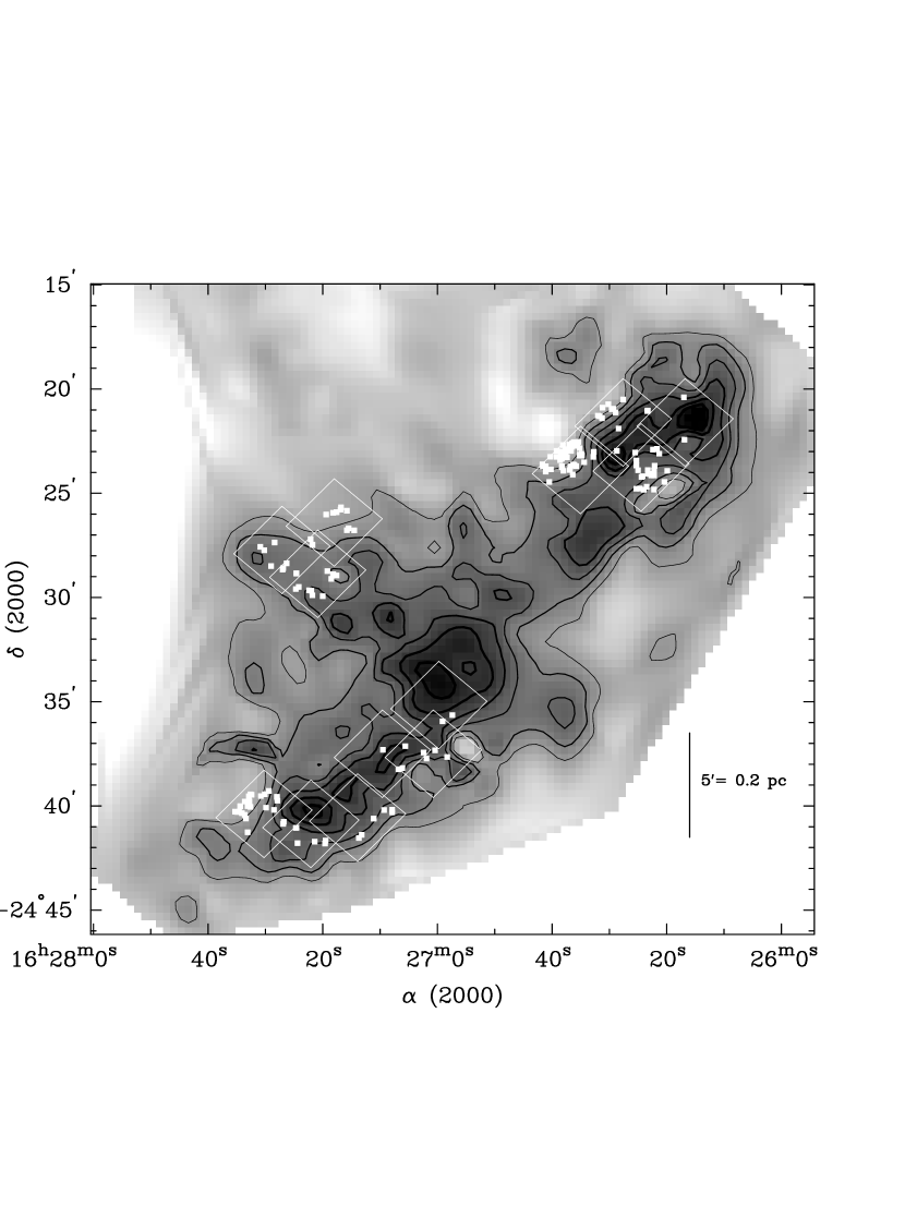
Figure 2: Extinction map, reproduced from Wilking & Lada (1983). Contours are plotted for $\rm{A_{V}}=$40-90 mag, at 10 mag intervals. Solid squares show the positions of the 165 sources detected at F160W. The regions covered by the HST survey are outlined, each box representing a $3\times 3$ mosaic.

In Figure 2, we reproduce the extinction map made by Wilking & Lada (1983), based on observations of C¹⁸O (J=1–0) and ¹²CO (J=1–0). On it we plot the locations of all 165 sources detected at F160W. Our HST mosaics are coincident with high $\rm{A_{V}}$ regions, with the exception of some fields on the eastern sides of cores A, B, and F. These fields coincide with a steep gradient in the cloud column density, and in them large numbers of stars are seen. As the extinction increases toward the center of the cloud, the number of stars decreases. Clearly, a significant fraction of detected sources on the edges of the cloud cores must be background stars.

The infrared Galactic model of Wainscoat et al. (1992) predicts the existence of approximately 140 stars arcmin^-2 brighter than our detection limit in the direction of the Ophiuchus cloud, assuming $\rm{A_{V}}=0$. However, when the model prediction is convolved with the $\rm{A_{V}}$ map, the resulting background is substantially smaller. This was done by calculating the expected background for each pixel in the $\rm{A_{V}}$ map, then summing over all pixels to obtain the total number of expected background stars as a function of H magnitude.

In Figure 3 we plot the observed H-band distribution of stars (using the conversion from magnitude at F160W to magnitude at H given in Section 2.3). The distribution predicted by Wainscoat’s model and reddened with our $\rm{A_{V}}$ map (assuming $\rm{A_{H}}$ = 0.155$\rm{A_{V}}$, Cohen et al. (1982)) is shown as a heavy dotted line. It appears that the background is small, becoming dominant only for H$>$20 mag. For comparison, we also plot the expected background as seen through a uniform extinction cloud of $\rm{A_{V}}=$ 35, 40, and 45 mag. The background modelled with our extinction map agrees closely with that for a uniform extinction of 40 mag. For this reason, we shall assume that all stars lying outside the $\rm{A_{V}}=$40 mag. contour in Figure 2 are background. Within the 40 mag. contour, the probable number of background stars given by the Wainscoat model ranges from approximately 0.50 stars arcmin^-2 (for $\rm{A_{V}}$=40 mag) to 0.02 stars arcmin^-2 (for $\rm{A_{V}}$=80 mag). Of the 165 sources detected in our survey, 108 sources lie within the 40 mag contour, and 58 of these are new detections, too faint to have been detected in previous surveys. In the discussions of clustering, multiplicity, and brown dwarfs which follow, only these 108 sources will be considered.

3.2 The spatial distribution of young stars in the Ophiuchus cloud

Ground–based imaging surveys at 2 $\mu$m revealed that the young stars in the Ophiuchus cloud are clustered in 3–4 main groups associated with dense cores of molecular gas (Luhman & Rieke, 1999; Barsony et al., 1997; Strom, Kepner & Strom, 1995; Comeron et al., 1993; Greene & Young, 1992; Barsony et al., 1989; Rieke, Ashok, & Boyle, 1989). Our HST survey targeted these peaks in the YSO surface density distribution, allowing us to examine structure within these stellar concentrations to a greater depth and with higher resolution than before.

The highest concentration of sources is in core A, where 23 stars are detected at F160W within an area $0.08\times 0.05$ pc in size (1$\farcm$9 x 1$\farcm$2 , centered on HST position 2 in Table 1). The extinction in this area is $\rm{A_{V}}=45-80$ mag, and averages 60 mag, leading to an estimated background contribution of 0.3$\pm$2 stars. The YSO surface density in the area, excluding background objects, is then $\sim 5\times 10^{3}$ stars pc^-2. Assuming a range of depths from half to twice the area width, we estimate stellar volume densities of $\sim 4-10\times 10^{4}$ stars pc^-3, comparable to the density of $2\times 10^{4}$ stars pc^-3 determined for the core of the Orion nebula cluster (Hillenbrand & Hartmann 1998). Other peaks in the stellar density are found in core B (HST positions 9 and 10) and core E (HST positions 12 and 13). Volume densities there are slightly less, ranging from $0.6-5\times 10^{4}$ stars pc^-3.

Inverting the volume density yields a mean spacing between stars in the core A peak of $0.02-0.03$ pc, or $\sim 4000-5000$ AU, and $\sim 5600-11000$ AU in the B and E cores. This is similar to the 6000 AU “fragmentation” scale identified by Motte et al. (1998) in their analysis of 1.3 mm continuum dust clumps, which are concentrated in the same three regions as the infrared sources reported here.

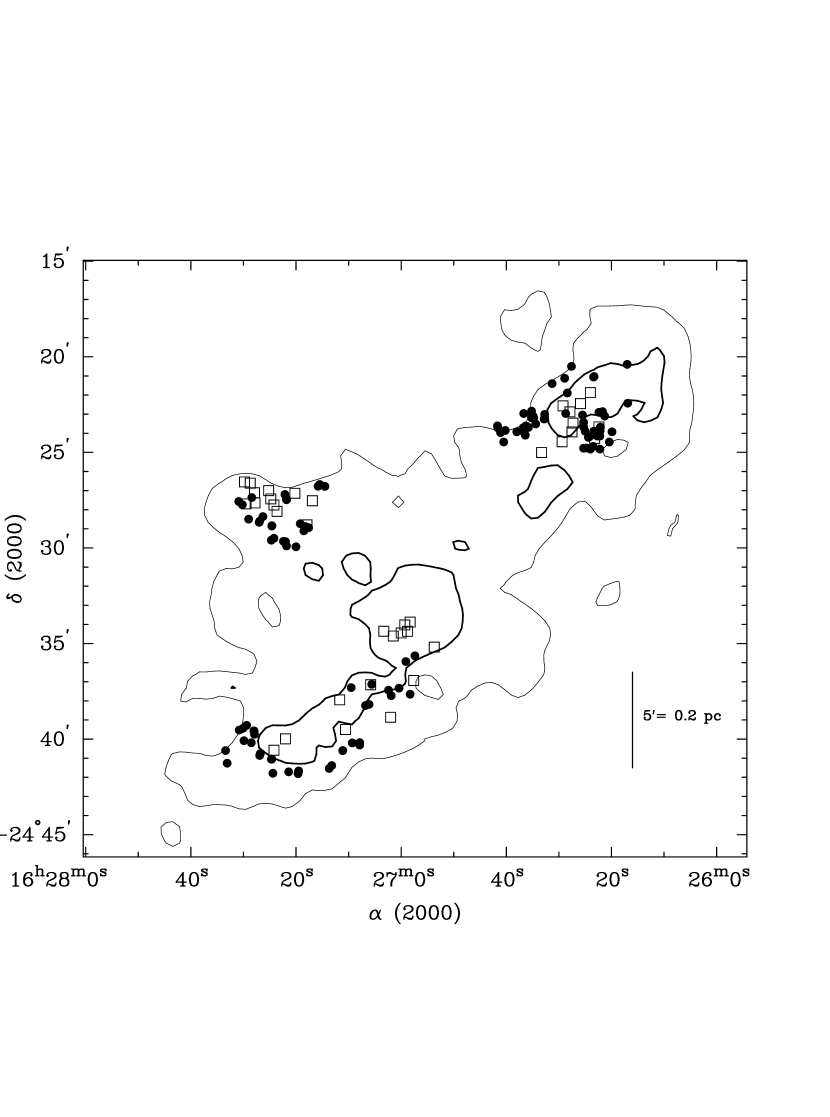
Figure 4: Spatial distribution of the HST sample (filled circles) and starless dust clumps from Motte et al. (1998) (open squares). Contours show $\rm{A_{V}}=$40 and 70 mag. Note how the starless clumps appear to be preferentially located in regions of higher extinction.

In fact, the embedded stars in Ophiuchus and the dust clumps detected at 1.3 mm have similar, but not identical, spatial distributions. The clumps show the same sub-clustering shown by the stars, as seen in Figure 4, where the positions of the starless clumps from Motte et al. (1998; open squares) have been plotted along with the positions of the stars (filled circles). Interestingly, the clumps are more strongly associated with the highest extinction regions of the cloud, whereas the stars appear to cluster around the edges of these regions.

This similar spatial relation of the stars and the millimeter continuum clumps in each of the three subgroups of the Ophiuchus core suggests that we are observing a real effect with the same explanation (origin?) in each subgroup. Some of the millimeter continuum clumps could be highly extincted YSOs, but this seems unlikely because most of the clumps are extended, some have associated compact molecular line emission, and the necessary extinction, $\rm{A_{V}}>1000$ mag, is in all other known cases accompanied by emission at far- and mid-infrared wavelengths (cf. Ladd et al. 1991). Adopting the interpretation of Motte et al. (1998) that the millimeter continuum clumps are prestellar, a more likely explanation is that in each subgroup, the region of highest extinction is a “starless core” which has not yet formed stars, but has formed numerous protostellar condensations with relative spacing (4000-5000 AU) similar to that of the surrounding young stars. In this picture, the similar spacing of prestellar and young stellar objects suggests that the young stellar objects have neither concentrated nor dispersed significantly since their formation. This evidence for spatial segregation by age may offer important clues to how stars form in clusters.

3.3 Multiplicity and clustering

To search for apparent binary pairs and higher-order multiple systems, we performed both a visual examination of all images and a nearest neighbor calculation for all detected sources. However in order to decrease the likelihood of mistaking background stars for companions, we restricted the sample to the 108 stars projected within the $\rm{A_{V}}\geq$40 mag contour of the cloud (as discussed in § 3.1).

For relatively faint stars (m(F160W)$\geq$18), our survey is sensitive to separations comparable to the resolution of the array (0$\farcs$2 pixel^-1), although due to the complex NICMOS PSF, our detection of faint companions within $\theta<0.5$″  of bright stars may be incomplete. To guard against bias, we took our estimated limiting magnitude for faint companions (m(F160W)$\geq$18) and imposed this limit on the sample, further restricting our sample to 62 stars. The maximum separation considered in our search was 10″(1450 AU), chosen to coincide with previous searches for pre-main sequence binaries. Within the separation range of 0$\farcs$2 to 10″, we detected seven apparent binary pairs and six apparent triple systems. They are listed in Table 3, and shown in Figure 5. The triple systems pictured in panels i, j, and k in Figure 5, are unusual in that they appear to be non-hierarchical. The other triple systems reported here (panels l and m) are organized in the usual way, having a close pair with a widely separated third member.

The multiplicity fraction, defined as the ratio of the number of binary and multiple systems detected, to the number of single, binary and multiple systems observed, or mf=B+M/(S+B+M), is then 0.30$\pm$0.08. Several previous multiplicity studies have included targets in Lynds 1688, each one sensitive to a specific range of companion separations and limiting magnitudes. In the lunar occultation experiment of Simon et al. (1995), observations were sensitive to stars brighter than K$\sim$11 and binary separations of 0$\farcs$005  to 10″.  Observing 35 systems, they detected 10 binaries, two triples, and one quadruple, for a multiplicity fraction of 0.37$\pm$0.10.

There are important differences between Simon et al. (1995; hereafter S95) and this study which should be considered when comparing their results. First, the minimum separation detectable by S95 was 0$\farcs$005, whereas ours is $\sim$0$\farcs$2. The limiting magnitude of the samples also differ: $\rm{K_{lim}}\sim 12$ and $\rm{H_{lim}}=18$ in S95 and this study, respectively. For projected separations between 0$\farcs$2  and 10″  only, S95 obtain mf$\sim 0.26\pm 0.08$. When we compare this with our mf of $0.30\pm 0.08$ for a deeper limiting magnitude, we conclude that the two results do not differ significantly. Within the uncertainties, the multiplicity fractions of S95 and this work are in agreement.

The relationship between the separation of binary pairs and clustering on a larger scale has been explored in a number of nearby star forming regions, including Ophiuchus (Ghez, Neugebauer, & Matthews, 1993; Reipurth & Zinnecker, 1993; Strom, Kepner & Strom, 1995; Nakajima et al., 1998). Of particular interest is the mean surface density of companions (MSDC), which Larson (1995) applied to young stars in the Taurus-Auriga star-forming region, finding clustering on two distinct scales. For large-scale clustering the MSDC was found to have a power-law slope of $\approx$ $-0.6$, and for small separations a slope of $\approx$ $-2$ was found. The “break point” between large and small scale slopes was determined to be $\approx$ $0.04$ pc. Simon (1997; hereafter S97) computed the MSDC for Ophiuchus, Taurus, and the Trapezium, finding similar power laws for each.

We computed the MSDC for the 108 stars projected within the $\rm{A_{V}}\geq$40 mag contour of Figure 2. The result is shown in Figure 6 for two samples of different depths: a shallow magnitude cutoff (H$\leq$14) and a deep limiting magnitude (H$\leq$21). As seen in Figure 6, the two samples have different break points. The shallow magnitude limit was selected to approximately match that of S97 (K$\leq$12), and not surprisingly, the two MSDCs have the same slopes and break points. The deeper sample shows a break point on a smaller spatial scale (by an order of magnitude). Thus, in a given star forming region, the properties of the MSDC can vary according to the depth of the sample. Bate et al. (1998) cautioned against overinterpreting the MSDC, in part for this reason. We offer this comparison as further caution.

3.4 New candidate brown dwarfs

With completeness limits of 21.5 and 21.0 magnitudes at F110W and F160W respectively, our survey is sensitive to very low-mass objects. For example, we should have detected stars of spectral type L4 V, through as much as 17 $\rm{A_{V}}$, assuming $\rm{M_{J}}=13.2$ and $\rm{M_{H}}=12.3$ (Kirkpatrick et al., 1999). Such very low-mass objects are relatively “blue” in intrinsic color, typically having $\rm{(J-H)<2}$ (Kirkpatrick et al. 1999), and so might be distinguishable from heavily reddened background stars in an infrared color-magnitude diagram.

Using the transformations from F110W and F160W to J and H listed in § 2.3 and the fluxes in Table 2, we converted our measured magnitudes to J and H magnitudes and plotted them in the color-magnitude diagram shown in Figure 7. Also plotted are the $3\times 10^{5}$ yr isochrone and the ZAMS from the pre-main sequence stellar evolution models of D’Antona & Mazzitelli (1997). Only the 65 sources detected in both the F110W and F160W bands are shown.

Brown dwarfs cannot be positively identified using near-IR photometry alone. However, those sources which are faint and relatively blue are more likely to be low-mass objects in the cloud than background stars seen through the cloud, especially if they are coincident with high extinction regions. We identified ten candidate brown dwarfs in our sample, using the following criteria: i) (J-H)$<$ 3.0, ii) J$>$15, and iii) position coincident with cloud extinction values of $\rm{A_{V}}>50$ mag. Spectral types have been published for three of these objects. One object, 162622$-$242409 is almost certainly sub-stellar, having been assigned a spectral type of M6.5 by both Wilking, Greene, & Meyer (1999; hereafter WGM) and Luhman & Rieke (1999; hereafter LR), and having a luminosity of 0.002-0.003 $\rm L_{\odot}$. The mass of object 162622$-$242354 is less certain. WGM classify it as M8.5 with $\rm L_{bol}\sim 0.004L_{\odot}$, whereas LR adopt a spectral type of M6.5 and a luminosity of 0.067 $\rm L_{\odot}$. The third classified object, 162659$-$243556, is a star of type M4 (LR), too hot to be a brown dwarf. The remaining seven (new) brown dwarf candidates are noted in Table 2. They are located in core A, which contains the highest density of stars in the survey (§ 3.1). Two of the candidates, 162622$-$242409 and 162622$-$242408, are members of triple systems (§ 3.3 and Table 3). One of the candidates, 16265$-$242303, is just on the red edge of our color criterion, but qualifies for selection when photometric uncertainties are taken into account.

There are a total of ten known brown dwarfs in the Ophiuchus cluster (LR, WGM) and another five sources known to occupy the transition region in the HR diagram between the stellar and substellar regimes (WGM). If all of the seven new candidates identified here are indeed substellar, the number of brown dwarfs known in the Ophiuchus cluster will have increased by 50%-70%. We can assess the implications for the stellar initial mass function (IMF) in the cluster. However, because fainter, lower-mass objects cannot be seen as deeply into the cloud as higher-mass stars, we restrict our analysis to an extinction-limited sample. In Figure 7, there are 30 sources within an extinction-limited region delimited by the $3\times 10^{5}$ yr isochrone and the $\rm{A_{V}}<20$ mag limit. These include our seven new candidate brown dwarfs, and the two confirmed brown dwarfs. If all seven of the new candidates are brown dwarfs, the total fraction of substellar objects in the extinction-limited sample is 9/30 = 30%. This is consistent with the results of LR, who argued that the IMF includes a large fraction of sub-stellar mass objects.

4 Morphologies of extended sources

Several interesting extended objects were covered by our survey, including the well-known infrared sources GSS 30, YLW 15A and YLW 16A, as well as some catalogued objects whose morphologies were previously unresolved. These sources are shown in Figure 8 and described in detail below.

GSS 30 (162621$-$242306): This multiple source is perhaps the most studied object in Ophiuchus. The illuminating star GSS 30–IRS 1 (162621$-$242306) is a class I source of unknown spectral type. A K-band spectrum obtained by LR showed the source to be heavily veiled (r$>$2) with no photospheric absorption features, and with Br$\gamma$ in emission. Two other infrared sources, GSS 30–IRS 2 and GSS 30–IRS 3, are located within the projected bounds of the nebula.

The nebula illuminated by IRS 1 has itself been the subject of many investigations. Near-infrared polarimetry images (Chrysostomou et al., 1997, 1996; Weintraub et al., 1993; Tamura et al., 1991; Castelaz et al., 1985) delineate a bipolar morphology coincident with the near-IR emission on the northeast side, and extending to the southwest side, where there is less infrared emission. The polarization pattern is approximately centrosymmetric around the illuminating source, and shows a “polarization disk” orthogonal to the long axis of the nebula. Zhang et al. (1997) detected a somewhat flattened molecular core in C¹⁸O and ¹³CO (J=1–0), in roughly the same orientation as the polarization disk. In the high resolution image presented in Figure 8 one sees the characteristic hourglass morphology of a bipolar nebula. The emission is dominated by the northeast lobe, a fact which has led previous investigators to propose that the fainter southwest lobe is obscured by a tilted circumstellar disk or toroid (Castelaz et al., 1985; Tamura et al., 1991; Weintraub et al., 1993; Chrysostomou et al., 1997).

GSS 30–IRS 2 (162622$-$242254) is a class III source of late K/early M spectral type (Luhman & Rieke, 1999; Greene & Meyer, 1995), located 20″  to the northeast of GSS 30–IRS 1. Its relatively advanced evolutionary class indicates it is probably unrelated and slightly foreground to the nebula.

GSS 30–IRS 3 (162621$-$242251) is a class I source of unknown spectral type, 15″  to the northeast of GSS 30–IRS 1, and 11″  southwest of GSS 30–IRS 2. This source has an extended point spread function and a crescent-shaped morphology. In addition, the F160W image shows a patch of obscuration (about an arcsecond in size) adjacent to the emission peak. Thus it is likely that the emission we see is scattered light from an embedded source. GSS 30–IRS 3 is also a strong radio source (LFAM 1), with emission at 6 cm (Leous et al., 1991).

GY 30 (162625$-$242303): Fan-shaped nebulosity extends to the east of this apparently low-mass object.

(162704$-$243707): Detected only at F160W, this source has a bipolar morphology strongly suggestive of a YSO outflow cavity, similar to that seen in GY 244, but fainter. This source was reported in Brandner et al. (2000), who imaged it at 2.2 $\mu$m.

WL 15 (162709$-$243718): WL 15 (Elias 29) is a class I source (Wilking, Lada, & Young, 1989) with a molecular outflow (Bontemps, et al., 1996; Sekimoto et al., 1997). The near-IR spectrum of El 29 resembles that of GSS 30–IRS1; a heavily veiled, featureless spectrum with the Br $\gamma$ line in emission (Luhman & Rieke, 1999).

Simon et al. (1987) found that the best fit to their lunar occultation observations was a two-component model having a central 7 mas component producing most of the emission at 2.2 $\mu$m and a larger component 0$\farcs$4  in extent, roughly centered on the smaller one. Our F160W image is consistent with this. The source is slightly elongated and has a measured FWHM of 0$\farcs$33  (3.3 pixels in our dithered image).

GY 244 (162717$-$242856): This source has a class I spectral energy distribution (Wilking, Lada, & Young, 1989), and a K-band spectral type of M4 (Luhman & Rieke, 1999). Our images show a bipolar nebula associated with this source. The morphology of the nebula is characteristic of the scattered light seen from YSO outflow cavities (Whitney & Hartmann, 1992) and suggests that the SW lobe is inclined somewhat toward us. Faint nebulosity in the F160W image indicates that the stars near GY 244 (GY 246, GY 247, and GY 249) also have some circumstellar envelope material associated with them.

(162724$-$244102): Detected only at F160W, this source has a faint bipolar morphology similar to that of (162704$-$243707). Also reported in Brandner et al. (2000).

YLW 15A (162726$-$244051): This embedded source has a heavily veiled, featureless 2 $\mu$m spectrum (Luhman & Rieke, 1999). It is included in our list of binary systems (Table 3), on the basis of a companion located $\sim$6″  to the northwest.

YLW 16A (162728$-$243934): We detect two non-point sources at the position of YLW 16A, separated by 0$\farcs$5  (position angle  270°). The flux ratio of the two peaks is 1.5 at 1.1 $\mu$m and 1.1 at 1.6 $\mu$m, with a large uncertainty due to the extended nature of the sources. As both of these sources are extended, it unclear whether they are actually two embedded stars, or a single embedded star seen in scattered light; possibly a star/disk/envelope system.

The appearance of the two peaks is more diffuse at 1.1 $\mu$m than at 1.6 $\mu$m, as would be expected if the light we detect is mainly scattered light. In addition, the flux ratio is greater at 1.1 $\mu$m than at 1.6 $\mu$m, suggesting differential reddening to the two peaks. Lunar occultation observations at 2 $\mu$m of YLW 16A (Simon et al., 1987) failed to resolve this source as a binary, instead showing it to be a single extended source of size (at K) $\sim$0$\farcs$5, which is the angular separation of the two peaks observed in our HST images. Thus it is possible that YLW 16A is a single star+disk+envelope, rather than an embedded binary system.

GY 273 (162728$-$242721): Large sigma-shaped nebula. It is unclear from our images where the illuminating source is.

5 Summary

We have presented a NICMOS 3 survey in the F110W and F160W filters of the dense star-forming cores of the Ophiuchus molecular cloud. Among our results:

1. The number of sources detected at F160W is 165, of which 65 were detected at F110W. Based on a search of the literature, we estimate that approximately two-thirds of the sources detected at F160W were previously uncatalogued. Of the 108 sources located within the $\rm{A_{V}}=$40 mag. contour of the cloud, 58 were previously uncatalogued.

2. The Ophiuchus star forming region has multiple peaks in stellar density. In core A we measure ${\rm n_{\ast}=4\times 10^{4}\,stars\,pc^{-3}}$ within a volume 0.05-0.08 pc on a side, and in cores B and E, ${\rm n_{\ast}=0.6-5\times 10^{3}\,stars\,pc^{-3}}$ within similar volumes. Such densities are similar to those seen on larger scales in rich clusters such as the Orion Nebula cluster.

3. Thirteen apparent multiple systems (eight binary pairs and five triples) with projected separations in the range 0$\farcs$2  to 10″  (29 to 1450 AU) were detected.

4. Seven new candidate brown dwarfs were identified from their positions in a color-magnitude diagram. According to our analysis of an extinction-limited sample, sub-stellar mass objects may account for as many as 30% of the sources in the core of the Ophiuchus cluster.

5. The unprecedented combination of resolution and sensitivity provided by HST has revealed new structures in the infrared sources in Ophiuchus. Bipolar structure is clearly seen in five objects.

Figure 1: Locations of observed fields shown on an optical (DSS) image of the Ophiuchus main cloud. Each of the 13 fields is $2\farcm 45\times 2\farcm 45$ in size, and is composed of a $3\times 3$ mosaic of NICMOS-3 fields. Coordinates of the 13 fields are listed in Table 1, along with core designations (A,B,E,F) after Loren et al. 1990.

Figure 3: Observed distribution of H magnitudes. The vertical dashed line shows the H-band completeness limit, and the heavy dotted line shows the predicted background, using Wainscoat’s infrared Galaxy model and the $\rm{A_{V}}$ map shown in Figure 2. Model background populations assuming uniform extinction of 35, 40, and 45 $\rm{A_{V}}$ are shown for comparison. The hatched part of the histogram represents stars whose projected locations on the cloud correspond to $\rm{A_{V}}\leq$ 40 mag.

Figure 5: F160W band images of binary (a-h) and multiple (i-m) sources, as identified in Table 3. Very faint companions are encircled. The bright primaries in panels (l) and (m) are themselves doubles (see Table 3). Each image is 12″  on a side.

Figure 6: Surface density of stars in the Ophiuchus sample, as a function of source separation. The break in slopes distinguishing the “cluster” or “field” distribution from the “binary” distribution depends on the depth of the sample. Distributions are shown for this study, H$\leq$21 (filled circles) and H$\leq$14 (open circles); and for Simon (1997). Larson’s (1995) power–law fits are plotted as a dashed line for the larger separations ($\Sigma\propto\Theta^{-0.62}$) and a solid line for separations less than 0.04 pc ($\Sigma\propto\Theta^{-2.15}$).

Figure 7: Color-magnitude diagram for the 65 sources detected within the estimated completeness limits in both the F110W and F160W bands. Magnitudes have been transformed from F110W and F160W to the J, H (CIT) system using the transformation relations in Section 2.3. Ten sources satisfying our criteria for brown dwarf candidacy are distinguished by their point types. The sources 162622$-$242409 (sub-stellar) and 162622$-$242354 (possibly sub-stellar) are plotted as open squares, and the type M4 star 162659$-$243556 as an open triangle. The seven new brown dwarf candidates from this study are represented as solid triangles. Error bars represent 1$\sigma$ internal photometry errors.

Figure 8: Extended sources described in section 4. Clockwise from top left: GSS 30; GY244$+$GY247$+$GY246; WL 15; GY30; 162724$-$244102; 162704$-$243707; YLW 16A; GY 273; YLW15A. Images in the F110W and F160W filters were combined to produce these false color images, except for 162724$-$244102 and 162704$-$243707, which were detected at F160W only.

Table 1: Fields Observed

Field	R.A.	Dec.	Core
1	16:26:16.0	-24:21:30	A
2	16:26:23.0	-24:23:40	A
3	16:26:25.0	-24:21:30	A
4	16:26:32.0	-24:23:40	A
5	16:26:59.0	-24:35:10	E
6	16:26:59.0	-24:37:30	E
7	16:27:08.0	-24:37:30	E
8	16:27:18.0	-24:26:20	B
9	16:27:21.0	-24:28:50	B
10	16:27:27.0	-24:27:40	B
11	16:27:14.0	-24:40:30	F
12	16:27:22.0	-24:40:40	F
13	16:27:30.0	-24:40:10	F

.

Table 2: Photometry

ID	R.A.	Dec.	m160	m110	cross-ref
162616$-$242225	16:26:16.9	-24:22:25	10.30 $\pm$ 0.00	11.13 $\pm$ 0.00	GSS29,SKS1-8
162617$-$242023	16:26:17.0	-24:20:23	9.17 $\pm$ 0.00	9.86 $\pm$ 0.00	DoAr24,SKS1-9
162619$-$242355	16:26:19.9	-24:23:55	18.07 $\pm$ 0.11	21.42 $\pm$ 0.47	$\cdots$
162620$-$242427	16:26:20.4	-24:24:27	17.77 $\pm$ 0.09	21.24 $\pm$ 0.40	$\cdots$
162621$-$242306	16:26:21.3	-24:23:06	10.59 $\pm$ 0.01	14.20 $\pm$ 0.03	GSS30,SKS1-12
162621$-$242251	16:26:21.7	-24:22:51	17.42 $\pm$ 0.09	$>$21.5	$\cdots$
162622$-$242340	16:26:22.1	-24:23:40	17.64 $\pm$ 0.09	$>$21.5	$\cdots$
162622$-$242354	16:26:22.2	-24:23:54	13.86 $\pm$ 0.01	16.47 $\pm$ 0.04	GY10,SKS1-14
162622$-$242449	16:26:22.2	-24:24:49	15.66 $\pm$ 0.03	19.98 $\pm$ 0.21	SKS3-12
162622$-$242409	16:26:22.2	-24:24:09	14.65 $\pm$ 0.02	16.94 $\pm$ 0.05	GY11,SKS3-13
162622$-$242254	16:26:22.4	-24:22:54	12.14 $\pm$ 0.00	15.72 $\pm$ 0.03	GY12
162622$-$242403	16:26:22.6	-24:24:03	17.66 $\pm$ 0.09	20.85 $\pm$ 0.31	$\cdots$
162622$-$242408	16:26:22.7	-24:24:08	15.79 $\pm$ 0.03	18.46 $\pm$ 0.10	$\cdots$
162623$-$242404	16:26:23.2	-24:24:04	19.70 $\pm$ 0.23	$>$21.5	$\cdots$
162623$-$242101	16:26:23.3	-24:21:01	8.76 $\pm$ 0.00	10.55 $\pm$ 0.00	DoAr24Ea
162623$-$242353	16:26:23.3	-24:23:53	17.90 $\pm$ 0.10	20.94 $\pm$ 0.34	$\cdots$
162623$-$242103	16:26:23.4	-24:21:03	10.47 $\pm$ 0.00	12.86 $\pm$ 0.00	DoAr24Eb
162623$-$242441	16:26:23.5	-24:24:41	12.23 $\pm$ 0.00	15.39 $\pm$ 0.02	LFAM3,SKS1-16
162624$-$242449	16:26:24.0	-24:24:49	8.76 $\pm$ 0.00	11.60 $\pm$ 0.00	S2,SKS1-17
162624$-$242410	16:26:24.2	-24:24:10	19.96 $\pm$ 0.28	$>$21.5	$\cdots$
162624$-$242412	16:26:24.4	-24:24:12	18.38 $\pm$ 0.13	$>$21.5	$\cdots$
162624$-$242446	16:26:24.7	-24:24:46	16.93 $\pm$ 0.07	21.06 $\pm$ 0.367	$\cdots$
162625$-$242353	16:26:25.0	-24:23:53	19.42 $\pm$ 0.21	$>$21.5	$\cdots$
162625$-$242325	16:26:25.3	-24:23:25	17.04 $\pm$ 0.07		SKS3-15
162625$-$242446	16:26:25.3	-24:24:46	13.19 $\pm$ 0.01	17.25 $\pm$ 0.06	GY29,SKS1-18
162625$-$242339	16:26:25.3	-24:23:39	20.64 $\pm$ 0.37	$>$21.5	$\cdots$
162625$-$242303	16:26:25.5	-24:23:03	14.45 $\pm$ 0.03	17.01 $\pm$ 0.15	GY30,SKS3-16
162627$-$242029	16:26:27.6	-24:20:29	19.41 $\pm$ 0.20	$>$21.5	$\cdots$
162628$-$242153	16:26:28.4	-24:21:53	15.30 $\pm$ 0.03	19.62 $\pm$ 0.45	GY38?,SKS69
162628$-$242258	16:26:28.7	-24:22:58	18.38 $\pm$ 0.12	$>$21.5	$\cdots$
162628$-$242107	16:26:28.9	-24:21:07	18.87 $\pm$ 0.16	$>$21.5	$\cdots$
162629$-$242056	16:26:29.3	-24:20:56	19.89 $\pm$ 0.26	$>$21.5	$\cdots$
162629$-$242057	16:26:29.6	-24:20:57	20.17 $\pm$ 0.30	$>$21.5	$\cdots$
162630$-$242043	16:26:30.2	-24:20:43	20.20 $\pm$ 0.30	$>$21.5	$\cdots$
162631$-$242053	16:26:31.2	-24:20:53	17.56 $\pm$ 0.08	21.05 $\pm$ 0.35	$\cdots$
162631$-$242124	16:26:31.3	-24:21:24	16.67 $\pm$ 0.05	20.05 $\pm$ 0.22	$\cdots$
162631$-$242118	16:26:31.7	-24:21:18	19.73 $\pm$ 0.25	$>$21.5	$\cdots$
162632$-$242116	16:26:32.0	-24:21:16	18.59 $\pm$ 0.14	$>$21.5	$\cdots$
162633$-$242300	16:26:33.0	-24:23:00	19.97 $\pm$ 0.27	$>$21.5	$\cdots$
162633$-$242315	16:26:33.1	-24:23:15	18.45 $\pm$ 0.13	21.74 $\pm$ 0.50	$\cdots$
162634$-$242330	16:26:34.7	-24:23:30	7.73 $\pm$ 0.00	9.46 $\pm$ 0.00	S1,SKS1-22
162635$-$242311	16:26:35.1	-24:23:11	20.62 $\pm$ 0.38	$>$21.5	$\cdots$
162635$-$242306	16:26:35.2	-24:23:06	20.31 $\pm$ 0.32	off field	$\cdots$
162635$-$242250	16:26:35.2	-24:22:50	19.47 $\pm$ 0.21	$>$21.5	$\cdots$
162635$-$242232	16:26:35.4	-24:22:32	20.19 $\pm$ 0.31	$>$21.5	$\cdots$
162635$-$242308	16:26:35.5	-24:23:08	19.88 $\pm$ 0.25	off field	$\cdots$
162635$-$242311	16:26:35.5	-24:23:11	18.48 $\pm$ 0.13	off field	$\cdots$
162635$-$242341	16:26:35.5	-24:23:41	20.19 $\pm$ 0.30	$>$21.5	$\cdots$
162635$-$242240	16:26:35.6	-24:22:40	20.85 $\pm$ 0.42	$>$21.5	$\cdots$
162635$-$242241	16:26:35.6	-24:22:41	19.94 $\pm$ 0.27	$>$21.5	$\cdots$
162635$-$242243	16:26:35.7	-24:22:43	20.94 $\pm$ 0.44	$>$21.5	$\cdots$
162635$-$242338	16:26:35.8	-24:23:38	21.20 $\pm$ 0.50	$>$21.5	$\cdots$
162636$-$242336	16:26:36.0	-24:23:36	17.46 $\pm$ 0.08	20.28 $\pm$ 0.24	$\cdots$
162636$-$242406	16:26:36.1	-24:24:06	15.95 $\pm$ 0.04	20.51 $\pm$ 0.28	GY76,SKS3-19
162636$-$242232	16:26:36.2	-24:22:32	20.95 $\pm$ 0.45	$>$21.5	$\cdots$
162636$-$242236	16:26:36.5	-24:22:36	19.64 $\pm$ 0.23	$>$21.5	$\cdots$
162636$-$242342	16:26:36.5	-24:23:42	19.41 $\pm$ 0.20	$>$21.5	$\cdots$
162636$-$242245	16:26:36.6	-24:22:45	19.98 $\pm$ 0.27	$>$21.5	$\cdots$
162636$-$242353	16:26:36.6	-24:23:53	16.19 $\pm$ 0.04	19.48 $\pm$ 0.17	SKS3-21
162636$-$242258	16:26:36.7	-24:22:58	19.89 $\pm$ 0.28	$>$21.5	$\cdots$
162637$-$242247	16:26:37.0	-24:22:47	18.03 $\pm$ 0.10	20.39 $\pm$ 0.26	$\cdots$
162637$-$242239	16:26:37.0	-24:22:39	17.59 $\pm$ 0.08	19.83 $\pm$ 0.19	$\cdots$
162637$-$242256	16:26:37.5	-24:22:56	20.51 $\pm$ 0.38	$>$21.5	$\cdots$
162637$-$242316	16:26:37.6	-24:23:16	18.24 $\pm$ 0.12	21.31 $\pm$ 0.40	$\cdots$
162637$-$242253	16:26:37.7	-24:22:53	19.37 $\pm$ 0.21	$>$21.5	$\cdots$
162637$-$242355	16:26:37.7	-24:23:55	19.88 $\pm$ 0.28	off field	$\cdots$
162637$-$242302	16:26:37.8	-24:23:02	12.68 $\pm$ 0.00	15.82 $\pm$ 0.03	GY81,SKS1-23
162638$-$242241	16:26:38.1	-24:22:41	16.59 $\pm$ 0.05	off field	$\cdots$
162638$-$242314	16:26:38.4	-24:23:14	20.44 $\pm$ 0.34	$>$21.5	$\cdots$
162638$-$242345	16:26:38.5	-24:23:45	18.55 $\pm$ 0.14	$>$21.5	$\cdots$
162638$-$242313	16:26:38.5	-24:23:13	20.67 $\pm$ 0.39	$>$21.5	$\cdots$
162638$-$242342	16:26:38.5	-24:23:42	20.25 $\pm$ 0.33	$>$21.5	$\cdots$
162638$-$242320	16:26:38.5	-24:23:20	23.81 $\pm$ 2.90	$>$21.5	$\cdots$
162638$-$242300	16:26:38.6	-24:23:00	20.73 $\pm$ 0.39	$>$21.5	$\cdots$
162638$-$242317	16:26:38.6	-24:23:17	20.58 $\pm$ 0.36	$>$21.5	$\cdots$
162638$-$242312	16:26:38.7	-24:23:12	19.15 $\pm$ 0.18	21.86 $\pm$ 0.51	$\cdots$
162638$-$242324	16:26:38.8	-24:23:24	13.15 $\pm$ 0.01	15.84 $\pm$ 0.03	GY84,SKS24
162639$-$242258	16:26:39.4	-24:22:58	25.30 $\pm$ 7.42	off field	$\cdots$
162639$-$242315	16:26:39.4	-24:23:15	19.70 $\pm$ 0.23	$>$21.5	$\cdots$
162640$-$242351	16:26:40.2	-24:23:51	19.80 $\pm$ 0.25	$>$21.5	$\cdots$
162640$-$242315	16:26:40.3	-24:23:15	16.44 $\pm$ 0.05	off field	$\cdots$
162640$-$242427	16:26:40.5	-24:24:27	18.25 $\pm$ 0.12	$>$21.5	$\cdots$
162641$-$242342	16:26:41.1	-24:23:42	19.22 $\pm$ 0.18	$>$21.5	$\cdots$
162641$-$242357	16:26:41.1	-24:23:57	20.25 $\pm$ 0.30	$>$21.5	$\cdots$
162641$-$242343	16:26:41.6	-24:23:43	19.29 $\pm$ 0.19	$>$21.5	$\cdots$
162641$-$242336	16:26:41.7	-24:23:36	18.57 $\pm$ 0.13	$>$21.5	$\cdots$
162657$-$243538	16:26:57.4	-24:35:38	15.18 $\pm$ 0.02	19.45 $\pm$ 0.166	SKS3-23
162658$-$243739	16:26:58.3	-24:37:39	18.05 $\pm$ 0.10	$>$21.5	CRBR51,SKS3-24
162659$-$243556	16:26:59.1	-24:35:56	13.91 $\pm$ 0.01	16.75 $\pm$ 0.048	SKS3-25
162700$-$243719	16:27:00.4	-24:37:19	20.89 $\pm$ 0.41	$>$21.5	$\cdots$
162701$-$243743	16:27:01.9	-24:37:43	20.04 $\pm$ 0.29	$>$21.5	$\cdots$
162702$-$243726	16:27:02.4	-24:37:26	10.93 $\pm$ 0.00	14.80 $\pm$ 0.019	WL16,SKS1-25
162704$-$243707	16:27:04.6	-24:37:07	17.59 $\pm$ 0.18	$>$21.5	$\cdots$
162706$-$243811	16:27:06.1	-24:38:11	14.90 $\pm$ 0.02	15.83 $\pm$ 0.03	GY201
162706$-$243814	16:27:06.8	-24:38:14	13.77 $\pm$ 0.01	18.64 $\pm$ 0.11	WL17,SKS3-27
162707$-$244011	16:27:07.9	-24:40:11	19.95 $\pm$ 0.27	$>$21.5	$\cdots$
162707$-$244018	16:27:07.9	-24:40:18	16.70 $\pm$ 0.05	21.28 $\pm$ 0.39	$\cdots$
162709$-$244011	16:27:09.3	-24:40:11	13.58 $\pm$ 0.01	17.58 $\pm$ 0.07	$\cdots$
162709$-$243718	16:27:09.5	-24:37:18	11.05 $\pm$ 0.00	16.51 $\pm$ 0.06	GY214,WL 15, El 29, SKS1-28
162711$-$244036	16:27:11.1	-24:40:36	13.03 $\pm$ 0.01	17.15 $\pm$ 0.05	$\cdots$
162711$-$243831	16:27:11.4	-24:38:31	15.29 $\pm$ 0.03	21.10 $\pm$ 0.04	$\cdots$
162713$-$244123	16:27:13.2	-24:41:23	12.53 $\pm$ 0.00	17.49 $\pm$ 0.06	$\cdots$
162713$-$244132	16:27:13.7	-24:41:32	19.54 $\pm$ 0.21	$>$21.5 $\pm$  $\cdots$	$\cdots$
162714$-$242646	16:27:14.5	-24:26:46	15.25 $\pm$ 0.03	20.52 $\pm$ 0.27	GY236,SKS3-34
162715$-$242640	16:27:15.5	-24:26:40	13.42 $\pm$ 0.01	18.28 $\pm$ 0.09	GY239,SKS3-36
162715$-$242646	16:27:15.8	-24:26:46	20.12 $\pm$ 0.28	$>$21.5	$\cdots$
162715$-$242550	16:27:15.8	-24:25:50	19.99 $\pm$ 0.27	$>$21.5	$\cdots$
162716$-$242540	16:27:16.8	-24:25:40	19.14 $\pm$ 0.18	$>$21.5	$\cdots$
162716$-$242546	16:27:16.9	-24:25:46	20.35 $\pm$ 0.33	$>$21.5	$\cdots$
162717$-$242856	16:27:17.6	-24:28:56	13.63 $\pm$ 0.02	18.04 $\pm$ 0.16	GY244,SKS1-32
162717$-$242554	16:27:17.6	-24:25:54	18.55 $\pm$ 0.14	$>$21.5	$\cdots$
162717$-$242554	16:27:17.6	-24:25:54	18.61 $\pm$ 0.14	$>$21.5	$\cdots$
162718$-$242853	16:27:18.2	-24:28:53	14.73 $\pm$ 0.02	20.59 $\pm$ 0.29	WL5,SKS1-33
162718$-$242555	16:27:18.2	-24:25:55	18.89 $\pm$ 0.16	$>$21.5	$\cdots$
162718$-$242906	16:27:18.5	-24:29:06	11.02 $\pm$ 0.00	14.26 $\pm$ 0.01	WL4,SKS1-34
162719$-$242844	16:27:19.2	-24:28:44	14.41 $\pm$ 0.02	19.15 $\pm$ 0.28	WL3,SKS3-38
162719$-$242601	16:27:19.4	-24:26:01	18.67 $\pm$ 0.14	$>$21.5	$\cdots$
162719$-$244139	16:27:19.5	-24:41:39	8.70 $\pm$ 0.00	9.79 $\pm$ 0.00	SR12,SKS1-35
162719$-$244148	16:27:19.6	-24:41:48	15.21 $\pm$ 0.03	16.20 $\pm$ 0.03	$\cdots$
162720$-$242956	16:27:20.0	-24:29:56	20.03 $\pm$ 0.27	$>$21.5	$\cdots$
162721$-$244142	16:27:21.4	-24:41:42	11.48 $\pm$ 0.00	15.18 $\pm$ 0.02	YLW13b,SKS1-36
162721$-$242728	16:27:21.8	-24:27:28	18.71 $\pm$ 0.14	$>$21.5	$\cdots$
162721$-$242953	16:27:21.8	-24:29:53	14.38 $\pm$ 0.02	20.09 $\pm$ 0.22	GY254,SKS3-40
162722$-$242940	16:27:22.0	-24:29:40	15.37 $\pm$ 0.03	19.94 $\pm$ 0.21	GY256,SKS3-41
162722$-$242712	16:27:22.1	-24:27:12	19.83 $\pm$ 0.25	$>$21.5	$\cdots$
162722$-$242939	16:27:22.4	-24:29:39	19.89 $\pm$ 0.26	$>$21.5	$\cdots$
162724$-$242929	16:27:24.2	-24:29:29	15.03 $\pm$ 0.02	19.84 $\pm$ 0.20	GY257,SKS3-43
162724$-$244147	16:27:24.4	-24:41:47	15.07 $\pm$ 0.02	19.00 $\pm$ 0.13	GY258,SKS3-42
162724$-$242851	16:27:24.6	-24:28:51	20.54 $\pm$ 0.36	$>$21.5	$\cdots$
162724$-$242850	16:27:24.6	-24:28:50	20.00 $\pm$ 0.27	$>$21.5	$\cdots$
162724$-$244102	16:27:24.6	-24:41:02	18.60 $\pm$ 0.14	$>$21.5	$\cdots$
162724$-$242935	16:27:24.7	-24:29:35	14.70 $\pm$ 0.02	18.93 $\pm$ 0.13	GY259,SKS3-45
162724$-$244103	16:27:24.7	-24:41:03	18.55 $\pm$ 0.14	$>$21.5	CRBR85,SKS3-44
162726$-$242821	16:27:26.3	-24:28:21	19.11 $\pm$ 0.18	$>$21.5	$\cdots$
162726$-$244045	16:27:26.8	-24:40:45	14.75 $\pm$ 0.02	18.54 $\pm$ 0.14	GY263,SKS3-48
162726$-$244051	16:27:26.9	-24:40:51	13.05 $\pm$ 0.01	18.22 $\pm$ 0.16	YLW15A,SKS3-49
162726$-$242835	16:27:26.9	-24:28:35	20.83 $\pm$ 0.40	$>$21.5	$\cdots$
162727$-$242839	16:27:27.0	-24:28:39	20.76 $\pm$ 0.39	$>$21.5	$\cdots$
162727$-$244048	16:27:27.1	-24:40:48	18.21 $\pm$ 0.12	$>$21.5	$\cdots$
162727$-$243944	16:27:27.9	-24:39:44	18.82 $\pm$ 0.15	$>$21.5	$\cdots$
162728$-$243934A:B	16:27:28.0	-24:39:34	12.62 $\pm$ 0.02	17.15 $\pm$ 0.18	YLW16A,SKS3-51
162728$-$242721	16:27:28.4	-24:27:21	12.44 $\pm$ 0.00	16.30 $\pm$ 0.03	GY 273,VSSG18,SKS1-39
162728$-$244011	16:27:28.5	-24:40:11	18.02 $\pm$ 0.10	$>$21.5	$\cdots$
162729$-$244005	16:27:29.9	-24:40:05	20.69 $\pm$ 0.37	$>$21.5	$\cdots$
162729$-$242829	16:27:29.0	-24:28:29	19.25 $\pm$ 0.19	$>$21.5	$\cdots$
162729$-$243917	16:27:29.4	-24:39:17	14.29 $\pm$ 0.02	18.28 $\pm$ 0.11	GY274,SKS3-54
162730$-$243926	16:27:30.1	-24:39:26	19.80 $\pm$ 0.25	$>$21.5	$\cdots$
162730$-$242744	16:27:30.2	-24:27:44	11.53 $\pm$ 0.00	15.53 $\pm$ 0.02	VSSG17,SKS1-40
162730$-$243931	16:27:30.8	-24:39:31	20.25 $\pm$ 0.32	$>$21.5	$\cdots$
162730$-$242734	16:27:30.9	-24:27:34	19.22 $\pm$ 0.19	$>$21.5	$\cdots$
162732$-$243928	16:27:32.4	-24:39:28	20.62 $\pm$ 0.37	$>$21.5	$\cdots$
162732$-$243926	16:27:32.6	-24:39:26	18.84 $\pm$ 0.15	$>$21.5	$\cdots$
162732$-$244002	16:27:32.6	-24:40:02	19.16 $\pm$ 0.18	$>$21.5	$\cdots$
162732$-$243947	16:27:32.8	-24:39:47	17.93 $\pm$ 0.10	$>$21.5	$\cdots$
162732$-$243932	16:27:32.9	-24:39:32	20.59 $\pm$ 0.36	$>$21.5	$\cdots$
162733$-$244115	16:27:33.1	-24:41:15	9.35 $\pm$ 0.00	11.93 $\pm$ 0.00	GY292,SKS1-43
162733$-$244000	16:27:33.1	-24:40:00	18.25 $\pm$ 0.12	$>$21.5	$\cdots$
162733$-$244036	16:27:33.4	-24:40:36	16.42 $\pm$ 0.05	$>$21.5	CRBR91
162733$-$244025	16:27:33.6	-24:40:25	20.87 $\pm$ 0.42	$>$21.5	$\cdots$
162733$-$243947	16:27:33.6	-24:39:47	20.23 $\pm$ 0.31	$>$21.5	$\cdots$
162734$-$244021	16:27:34.1	-24:40:21	20.70 $\pm$ 0.39	$>$21.5	$\cdots$
162734$-$244001	16:27:34.4	-24:40:01	19.25 $\pm$ 0.20	$>$21.5	$\cdots$
162734$-$244017	16:27:34.6	-24:40:17	20.57 $\pm$ 0.35	$>$21.5	$\cdots$
162735$-$244017	16:27:34.9	-24:40:17	18.33 $\pm$ 0.12	$>$21.5	$\cdots$
162735$-$244016	16:27:35.3	-24:40:16	20.82 $\pm$ 0.40	$>$21.5	$\cdots$

Table 3: Multiple Systems

$\rm{ID_{A}}$	$\rm{ID_{B}}$	$\rm{m160_{A}}$	$\rm{m160_{B}}$	separation(″)	P.A.(°)	$\rm{cross-ref_{A}}$	fig
			Binaries
162625$-$242446	162624$-$242446	13.2	16.9	9.0	274	GY29	(a)
162634$-$242330A	162634$-$242330B	7.7	–			S1
162636$-$242336	162636$-$242342	17.5	19.4	9.5	127		(b)
162707$-$244018	162707$-$244011	16.7	19.9	7.7	354		(c)
162717$-$242856	162718$-$242853	13.6	14.7	9.7	65	GY244	(d)
162722$-$242940	162722$-$242939	15.4	19.9	6.0	84	GY256	(e)
162724$-$242935	162724$-$242929	14.7	15.0	9.5	314	GY259	(f)
162726$-$244051	162726$-$244045	13.0	14.7	5.9	323	YLW15A	(g)
162728$-$243934A	162728$-$243934B	15.9	–	0.6	260	YLW16A	(h)
			Triples
162622$-$242409	162622$-$242408	14.6	15.8	7.5	88	GY11	(i)
	162622$-$242403		17.7	7.7	42
162622$-$242408	162622$-$242403	15.8	17.7	4.9	340		(j)
	162623$-$242404		19.7	8.6	57
162636$-$242336	162635$-$242338	17.5	20.2	3.4	228		(k)
	162635$-$242341		20.2	9.0	234
162715$-$242640A	162715$-$242640B	13.4		0.3	48	GY239	(l)
	162715$-$242646		20.1	7.3	145
162719$-$244139A	162719$-$244139B	8.7		0.3	96	SR 12	(m)
	162719$-$244148		15.2	8.8	166
	162727$-$244048		18.2	4.4	3

References

- Adams & Myers (2001) Adams, F.C. & Myers, P.C. 2001, ApJ, 553, 744
- Barsony et al. (1989) Barsony, M., Burton, M. G., Russell, A. P. G., Carlstrom, J. E., and Garden, R. 1989, ApJ, 346, L93
- Barsony et al. (1997) Barsony, M., Kenyon, S. J., Lada, E. A., and Teuben, P. J. 1997, ApJS, 112, 109
- Bontemps, et al. (1996) Bontemps, S., André, P., Terebey, S. and Cabrit, S. 1996, A&A, 311, 858
- Carpenter (2000) Carpenter, J. M. 2000, AJ, 120, 3139
- Castelaz et al. (1985) Castelaz, M. W., Hackwell, J. A., Grasdalen, G. L., Gehrz, R. D. and Gullixson, C. 1985, ApJ, 290, 261
- Chelli et al. (1988) Chelli, A., Zinnecker, H., Carrasco, L. Cruz-Gonzáles, I., and Perrier, C. 1988, A&A, 207, 46
- Chrysostomou et al. (1997) Chrysostomou, A., Ménard, F., Gledhill, T. M., Clark, S., Hough, J. H., McCall, A. and Tamura, M. 1997, MNRAS285, 750
- Chrysostomou et al. (1996) Chrysostomou, A., Clark, S. G., Hough, J. H., Gledhill, T. M.,McCall, A. and Tamura, M. 1997, MNRAS278, 449
- Cohen et al. (1982) Cohen, J.G., Elias, J.H., Frogel, J.A., and Persson, S.E. 1981, ApJ, 249, 502
- Comeron et al. (1993) Comeron, F., Rieke, G. H., Burrows, A., and Rieke, M. J. 1993, ApJ, 416, 185
- de Zeeuw et al. (1999) de Zeeuw, P. T., Hoogerwerf, R., de Bruijne, J. H. J., Brown, A. G. A., and Blaauw, A. 1999, AJ, 117, 354
- Duquennoy & Mayor (1991) Duquennoy, A. & Mayor, M. 1991, A&A, 248, 485
- Elias (1978) Elias, J. H. 1978, ApJ, 224, 453
- Fazio et al. (1976) Fazio, G. G., Wright, E. L., Zeilik, and Low, F.J. 1976, ApJ, 206, L165
- Fruchter & Hook (1997) Fruchter, A. S., and Hook, R. N. 1997, Proc. SPIE, 3164
- Ghez, Neugebauer, & Matthews (1993) Ghez, A. M., Neugebauer, G., and Matthews, K. 1993, AJ, 106, 2005
- Grasdalen, Strom, & Strom (1973) Grasdalen, G. L., Strom, K. M., and strom, S. E. 1973, ApJ, 184, L53
- Greene & Young (1992) Greene, T. P. and Young, E. T. 1992, ApJ, 395, 516
- Greene & Meyer (1995) Greene, T. P. and Meyer, M. R. 1995, ApJ, 450, 233
- Hillenbrand & Hartmann (1998) Hillenbrand, L. A. & Hartmann, L. W. 1998, ApJ, 492, 540
- Kirkpatrick et al. (1999) Kirkpatrick, J. D., Ried, I. N., Leibert, J., Cutri, R. M., Nelson, B., Beichman, C. A., Dahn, C. C., Monet, D. G., Gizis, J. E., and Skrutskie, M. F. 1999, ApJ, 519, 802
- Klessen et al (2000) Klessen, R. and so forth
- Leous et al. (1991) Leous, J. A., Feigelson, E. D., André, P., and Montmerle, T. 1991, ApJ, 379, 683
- Loren & Wootten (1986) Loren, R. B., and Wootten, A. 1986, ApJ, 306, 142
- Loren, Wootten & Wilking (1990) Loren, R. B., Wootten, A., and Wilking, B. A. 1990, ApJ, 365, 269
- Luhman & Rieke (1999) Luhman, K. L. and Rieke, G. H. 1999, ApJ, 525, 440
- Luhman (1999) Luhman, K. L. 1999, private communication
- Meyer et al. (2000) Meyer, M.R., Adams, F.C., Hillenbrand, L.A., Carpenter, J.M., and Larson, R.B. 2000, Protostars and Planets IV (University of Arizona Press, eds Mannings, V., Boss, A.P., Russell, S.S.), p. 121
- Myers (2000) Myers, P.C. 2000, ApJ, 530, L119
- Motte et al. (1998) Motte, F., André, P. and Neri, R. 1998, A&A, 336,150
- Nakajima et al. (1998) Nakajima, Y., Tachihara, K., Hanawa, T., and Nakano, M. 1998, ApJ, 497, 721
- Reipurth & Zinnecker (1993) Reipurth, B. & Zinnecker, H. 1993, å, 278, 81
- Rieke, Ashok, & Boyle (1989) Rieke, G. H., Ashok, N. M., and Boyle, R. P. 1989, ApJ, 339, L71
- Rieke (1999) Rieke, M. 1999, private communication
- Sekimoto et al. (1997) Sekimoto, Y., Tatematsu, K., Umemoto, T., Koyama, K., Tsuboi, Y., Hirano, N., and Yamamoto, S. 1997, ApJ, 489, L63
- Simon et al. (1987) Simon, M., Howell, R. R., Longmore, A. J., Wilking, B. A., Peterson, D. M., and Chen, W.-P. 1987, ApJ, 320, 344
- Simon et al. (1995) Simon, M., Ghez, A. M., Leinert, Ch., Cassar, L., Chen, W. P., Howell, R. R., Jameson, R. F., Matthews, K., Neugebauer, G., and Richichi, A. 1995, ApJ, 443, 625
- Simon (1997) Simon, M. 1997, ApJ, 482, L81
- Strom, Kepner & Strom (1995) Strom, K. M., Kepner, J., and Strom, S. E. 1995, ApJ, 438, 813
- Tamura et al. (1991) Tamura, M., Gatley, I., Joyce, R. R., Ueno, M., Suto, H., and Sekiguchi, M. 1991, ApJ, 378, 611
- Vrba et al. (1973) Vrba, F. J., Strom, K. M., Strom, S. E., and Grasdalen, G. L. 1975, ApJ, 197, 77
- Wainscoat et al. (1992) Wainscoat, R. J., Cohen, M., Volk, K.,Walker, H. J., and Schwartz, D. E. 1992, ApJS, 83, 111
- Weintraub et al. (1993) Weintraub, D. A., Kastner, J. H., Griffith, L. L., and Campins, H. 1993, AJ, 105, 271
- Whitney & Hartmann (1992) Whitney, B. A. & Hartmann, L. 1992, ApJ, 395, 529
- Wilking & Lada (1983) Wilking, B. A. and Lada, C. J. 1983, ApJ, 274, 698
- Wilking, Lada, & Young (1989) Wilking, B. A., Lada, C. J. and Young, E. T. 1989, ApJ, 340, 823
- Wilking, Greene, & Meyer (1999) Wilking, B. A., Greene, T. P., and Meyer, M. R. 1999, AJ, 117, 469
- Wilking (1999) Wilking, B. A. 1999, private communication
- Zhang et al. (1997) Zhang, Q., Wootten, A. and Ho, P. T. P. 1997, ApJ, 475, 713