KMT-2016-BLG-1107: A New Hollywood-Planet Close/Wide Degeneracy

Abstract

We show that microlensing event KMT-2016-BLG-1107 displays a new type of degeneracy between wide-binary and close-binary Hollywood events in which a giant-star source envelops the planetary caustic. The planetary anomaly takes the form of a smooth, two-day “bump” far out on the falling wing of the light curve, which can be interpreted either as the source completely enveloping a minor-image caustic due to a close companion with mass ratio $q=0.036$, or partially enveloping a major-image caustic due to a wide companion with $q=0.004$. The best estimates of the companion masses are both in the planetary regime ($3.3^{+3.5}_{-1.8}\,M_{\rm jup}$ and $0.090^{+0.096}_{-0.037}\,M_{\rm jup}$) but differ by an even larger factor than the mass ratios due to different inferred host masses. We show that the two solutions can be distinguished by high-resolution imaging at first light on next-generation (“30m”) telescopes. We provide analytic guidance to understand the conditions under which this new type of degeneracy can appear.

1 Introduction

Gould (1997) proposed a “Hollywood” strategy of searching for microlensing planets by “following the big stars”, which made use of the fact that planets normally betray their presence in microlensing events when the source star passes over, or very close to, a caustic generated by the planet. For low-mass planets (hence, small caustics), the probability for the source to pass over the caustic is therefore proportional to the size of the source, rather than of the much smaller caustic. Gould & Gaucherel (1997) showed that for “wide” ($s>1$) topologies, the excess magnification $\Delta A$ (relative to the case of a point lens without planetary companions) when the source fully envelops the caustic is

$$\Delta A\rightarrow{2q\over\rho^{2}}={2m_{p}\theta_{\rm E}^{2}\over M\theta_{*}^{2}},$$ (1)

i.e., exactly the same value as would be the case if the planet were isolated. Here, $q=m_{p}/M$ is the planet-host mass ratio, $s$ is the planet-host separation normalized to the Einstein radius $\theta_{\rm E}$, $\rho=\theta_{*}/\theta_{\rm E}$, $\theta_{*}$ is the angular source radius,

$$\theta_{\rm E}=\sqrt{\kappa M\pi_{\rm rel}};\qquad\kappa\equiv{4G\over c^{2}{\rm AU}}\simeq 8.14\,{{\rm mas}\over M_{\odot}},$$ (2)

and $\pi_{\rm rel}={\rm AU}(D_{L}^{-1}-D_{S}^{-1})$ is the lens-source relative parallax. If we adopt a threshold of detectability of, e.g., $\Delta A\gtrsim 0.1$, then we can rewrite Equation (1) as

$$m_{p}={\theta_{*}^{2}\Delta A\over 2\,\kappa\pi_{\rm rel}}\gtrsim 0.75M_{\oplus}\biggl{(}{\theta_{*}\over 6\,\mu{\rm as}}\biggr{)}^{2}\biggl{(}{\pi_{\rm rel}\over 0.1\,{\rm mas}}\biggr{)}^{-1},$$ (3)

where we have normalized to the angular source size of a typical clump giant and to the relative parallax of a typical disk lens. Hence, this approach is potentially sensitive to very low-mass planets, particularly because large stars are also bright (unless they are heavily extincted), meaning that the photometric precision is generally good.

The virtue of this approach was first illustrated by OGLE-2005-BLG-390, which was intensively monitored by the PLANET collaboration, leading to the detection of a $q\sim 8\times 10^{-5}$ planet, with estimated mass $m_{p}\sim 5\,M_{\oplus}$ (Beaulieu et al., 2006). This was only the third published planet, and still to this date, one of only seven microlensing planets with well-measured mass ratios in the range $q<10^{-4}$ (Udalski et al., 2018).

Nevertheless, this channel has been the subject of remarkably little systematic study. The first fundamentally new development was the discovery of a potential degeneracy between “Cannae” and “von Schlieffen” Hollywood events, in which the source, respectively, fully and partially envelops the caustic (Hwang et al., 2018).

Here we analyze the Hollywood microlensing event KMT-2016-BLG-1107 and report the discovery a second potential (“close/wide”) degeneracy. Although this degeneracy has a similar $s\leftrightarrow s^{-1}$ symmetry to the well-established “close/wide” degeneracy that affects central caustics (Griest & Safizadeh, 1998; Dominik, 1999), the two degeneracies are not fundamentally related. We study the general conditions under which this close/wide planetary-caustic degeneracy can arise and show that (in strong contrast to the close/wide central-caustic degeneracy), the mass ratios $q$ of the two degenerate solutions generically differ by a relatively large factor, with the $s<1$ solution having a more massive planet. In the present case, $q=4.0\times 10^{-3}$ and $q=3.6\times 10^{-2}$ for the $s>1$ and $s<1$ solutions, respectively. Finally, we show that imaging with adaptive optics (AO) cameras will be able to resolve the degeneracy at first light on next-generation (“30m”) telescopes.

2 Observations

KMT-2016-BLG-1107 is at (RA,Dec) = (17:45:40.26,$-26$:01:54.48) corresponding to $(l,b)=(2.5,1.5)$. It was discovered by applying the Korea Microlensing Telescope Network (KMTNet, Kim et al. 2016) post-season event finder (Kim et al., 2018a) to 2016 KMTNet data (Kim et al., 2018c). These data were taken on KMTNet’s three identical 1.6m telescopes at CTIO (Chile, KMTC), SAAO (South Africa, KMTS) and SSO (Australia, KMTA), each equipped with identical $4\,{\rm deg}^{2}$ cameras. The event lies in KMTNet field BLG18 with a nominal cadence of $\Gamma=1\,{\rm hr^{-1}}$. In fact, the cadence was altered from April 23 to June 16 ($7501<{\rm HJD}^{\prime}\equiv{\rm HJD}-2450000<7555$) to support the Kepler K2 C9 microlensing campaign (Gould & Horne, 2013; Henderson et al., 2016; Kim et al., 2018b). During this period, the cadence was reduced to $\Gamma=0.75\,{\rm hr^{-1}}$ for KMTS and KMTA, but remained at $\Gamma=1\,{\rm hr^{-1}}$ for KMTC. We note that KMTC data are affected by a bad column on the CCD and so often have significantly larger error bars than KMTS and KMTA data.

The great majority of observations were carried out in the $I$ band with occasional $V$-band observations made solely to determine source colors. All reductions for the light curve analysis were conducted using the pySIS implementation (Albrow et al., 2009) of difference image analysis (DIA, Alard & Lupton 1998). While the $V$-band data are sufficient to measure the color (Section 4), because the source is very red and there are many fewer $V$-band points than $I$-band, the $V$-band data do not place significant constraints on the modeling. Thus, we do not use them in the modeling.

2.1 Removal of Long-Term Trend

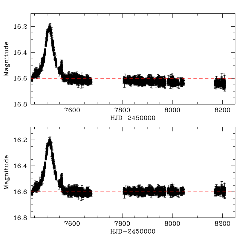
Figure 1: KMTC light curve of KMT-2016-BLG-1107 before (upper panel) and after (lower panel) removal of a linear trend in the baseline flux, which corresponds to $dI_{\rm base}/dt=+0.018\,{\rm mag\,yr^{-1}}$. The fit was done to 2017 data, while the extension to 2018 serves as a check. The slopes found for KMTA and KMTS are nearly identical.

The raw light curve shows a long-term trend in the combined 2016-2018 data. See Figure 1. The origin of this trend is unknown. It could, for example, be due to blended light from a relatively high-proper-motion nearby star. Whatever the cause, it is almost certainly unrelated to the primary microlensing event or the additional “bump” in the lightcurve. We therefore fit the baseline of the light curve to a constant plus a slope and remove the slope (see Figure 1) before undertaking the microlensing analysis.

3 Light Curve Analysis

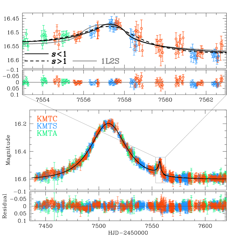
Figure 2: KMT-2016-BLG-1107 light curve, together with three models: “close binary lens” ($s<1$, solid black line), “wide binary lens” ($s>1$, dashed line) and “binary source” (1L2S, solid gray line). The upper panels show a zoom around the anomaly, while the lower panels show the full event. The residuals are calculated relative to the $s<1$ model. The 1L2S model is excluded by its failure to match the data on the rising wing of the anomaly at HJD${}^{\prime}=7556.xx$ as well as its overall high $\chi^{2}$. The close $(s<1)$ model is preferred by $\chi^{2}$ but this is an artifact of low-level variability, which depresses the data below either the $s<1$ or $s>1$ models by several sigma during the interval $7565<{\rm HJD}^{\prime}<7586$ during which the former model predicts very slightly lower magnification.

The resulting light curve of KMT-2016-BLG-1107 in the neighborhood of the event is shown in Figure 2. It primarily takes the form of a standard Paczyński (1986) single-lens/single-source (1L1S) curve, which is characterized by three geometric parameters $(t_{0},u_{0},t_{\rm E})$. These are, respectively, the time of maximum, the impact parameter (normalized to $\theta_{\rm E}$), and the Einstein timescale,

$$t_{\rm E}\equiv{\theta_{\rm E}\over\mu_{\rm rel}},$$ (4)

where ${\mbox{\boldmath$\mu$}}_{\rm rel}$ is the lens-source relative proper motion.

However, in addition there is a small, short-lived “bump” on the falling wing of the light curve at ${\rm HJD}^{\prime}\simeq 7557$. This appearance is qualitatively similar to the classic Hollywood event, OGLE-2005-BLG-390 (Beaulieu et al., 2006), and so plausibly could be generated by a similar major-image ($s>1$) caustic that is fully enveloped by the source. To test this conjecture, we conduct a systematic grid search over the seven standard parameters of binary-lens/single-source (2L1S) events. There are the three Paczyński (1986) parameters just mentioned $(t_{0},u_{0},t_{\rm E})$, the three parameters mentioned in Section 1, $(s,q,\rho)$, and the angle $\alpha$ between the binary axis and the direction of lens-source relative motion ${\mbox{\boldmath$\mu$}}_{\rm rel}$. In addition to these geometric parameters, there are two flux parameters $(f_{s},f_{b})$ for each observatory, $i$, so that the observed fluxes $F_{i}(t)$ are modeled by

$$F_{i}(t)=f_{s,i}A(t;t_{0},u_{0},t_{\rm E},\rho,s,q,\alpha)+f_{b,i}.$$ (5)

3.1 Two Solutions: Wide and Close Planetary Companions

We employ Monte Carlo Markov Chain (MCMC) $\chi^{2}$ minimization to carry out a grid search, in which $(t_{0},u_{0},t_{\rm E},\rho,\alpha)$ are allowed to vary, while $(s,q)$ are held fixed. The chains are seeded with $(t_{0},u_{0},t_{\rm E})$ derived from an initial Paczyński (1986) fit and $\rho=0.04$ based on the relative duration of the two bumps. For each $(s,q)$, $\alpha$ is seeded at six values that are spaced uniformly around the unit circle.

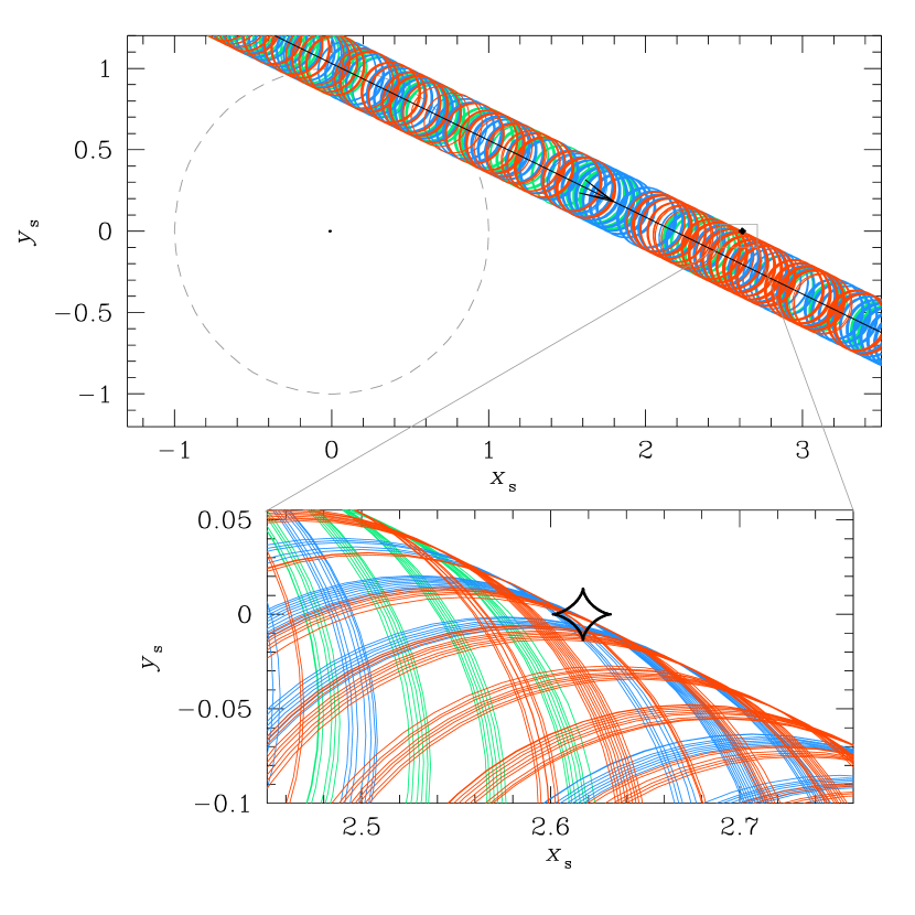
Figure 4: Caustic geometry of KMT-2016-BLG-1107, wide $(s>1)$ solution. The upper panel shows the source trajectory, which grazes the Einstein ring (dashed line) and then partially envelops the small quadrilateral planetary caustic, roughly 2.5 Einstein timescales $t_{\rm E}$ later. This von Schlieffen-type Hollywood envelopment is shown in greater detail in the lower-panel zoom, where the source position is shown by circles at the epochs of observations from the three color-coded observatories. This grazing geometry implies that the normalized source size $\rho$ must be substantially larger than for the close geometry (compare to Figure 3) in order to generate a “bump” of similar duration. This implies a substantially lower proper motion $\mu_{\rm rel}$, which will eventually permit future adaptive optics (AO) observations to distinguish between the two solutions. See Section 4 and, in particular, Equations (13) and (14).

The grid search yields only two minima whose geometries are shown in Figures 3 and 4. In both cases, the source passes over a small planetary caustic that lies far from the lens. For the solution with $s<1$, there are two such caustics, so we also check for a solution that crosses over the caustic at $(x_{\rm s},y_{\rm s})\sim(-2.4,1.0)$. This solution is disfavored by $\Delta\chi^{2}\sim 140$ of which $\Delta\chi^{2}\sim 50$ comes from the rising side of the light curve, when the source is forced to cross the ”de-magnified zone” even though no such demagnification is seen in the light curve. Furthermore, this solution has severe negative blending that makes it unphysical.

We further refine the two good solutions with additional MCMC runs, in which all seven parameters are allowed to vary. These two solutions are shown in Table 1. The flux values are quoted for the KMTC dataset. We note first that the Paczyński (1986) parameters $(t_{0},u_{0},t_{\rm E})$ are essentially identical between the two solutions. This is consistent with the fact that the light curve morphology is dominated by a broad bump that is generated by the host. Similarly, the flux parameters $(f_{s},f_{b})$ are also essentially identical.

Next we note that the two values of $s$, (0.345 and 2.96), almost perfectly obey $s\leftrightarrow s^{-1}$. The Paczyński (1986) curve is generated by two images, which lie at $u_{\pm}=(u\pm\sqrt{u^{2}+4})/2$, where $u$ is the projected lens-source separation normalized to $\theta_{\rm E}$. If the planet lies near either image, $s\sim|u_{\pm}|$, then it will perturb the image, giving rise to a short-lived deviation. Because $u_{-}=-u_{+}^{-1}$, it follows immediately that planetary deviations for close and wide solutions should be related by $s\leftrightarrow s^{-1}$.

The values of $\alpha$ differ substantially, but this mainly reflects that the major and minor images (and so any planet perturbing these images) lie on opposite sides of the host lens. In the limit $q\ll 1$, one expects $\alpha\leftrightarrow\pi-\alpha$ from this effect alone. However, this symmetry is broken at finite $q$ because the major-image caustic always lies directly on the binary axis whereas the two minor-image caustics are displaced from the axis by an angle that increases with $q$ (Han, 2006). These effects are apparent from examination of the caustic geometries, Figures 3 and 4.

The two really important differences between these solutions are in $q$ and $\rho$. The mass ratio $q$ is almost 10 times larger in the close solution while the normalized source size is more than three times smaller. Some insight into these differences is provided by Figures 3 and 4, which show the geometries of the two solutions.

In the close solution, the short-lived bump is caused by the complete (“Cannae”) envelopment of one of the two triangular caustics associated with minor-image perturbations, while in the wide solution it is caused by the partial (“von Schlieffen”) envelopment of the quadrilateral planetary caustic associated with major-image perturbations. In the latter geometry, the duration of the bump (which is an observed feature of the light curve) is substantially shorter than the diameter crossing time of the source, which immediately implies that the normalized source size must be substantially bigger than for the $s<1$ von Schlieffen solution.

3.2 Apparent Preference for Close Solution Is Not Real

We note that the close solution is nominally preferred by $\Delta\chi^{2}\simeq 40$. Under most circumstances, we would regard this as strong evidence in its favor. However, one can see from Figure 2 that the two models hardly differ, particularly compared to the error bars, which are relatively large ($\sim 0.006\,$mag for KMTS). We have investigated the origin of this apparently strong $\chi^{2}$ difference by constructing the cumulative distribution function of $\Delta\chi^{2}=\chi^{2}_{\rm wide}-\chi^{2}_{\rm close}$ as a function of time, and we find that most of the “signal” comes from $7565\lesssim{\rm HJD}^{\prime}\lesssim 7585$, i.e., when $\tau\equiv(t-t_{0})/t_{\rm E}$ is 3–4 Einstein timescales past peak. During this interval, the lightcurve is, on average, several $\sigma$ below either model. Under such conditions, $\Delta\chi^{2}\simeq 2\,(\delta/\sigma)((\Delta/\sigma)$ where $\delta$ is the difference between the models, $\Delta$ is the difference between the data and the mean of the two models, and $\sigma$ is the error bar. That is, for $\Delta/\sigma\sim 2.5$, we have $\Delta\chi^{2}=5(\delta/\sigma)$. In this way, many tens of points each contribute $\Delta\chi^{2}\sim 0.5$ even though the precision of the data does not permit them to distinguish between models. Inspecting the residuals in Figure 2, we see that they show irregular variability with an amplitude $\sim 0.02\,$ mag and a timescale of $\sim 20\,$days. Hence, we conclude that the apparent preference of the data for the close solution is an artifact of this low-level variability, i.e., that a degeneracy persists between the close and wide solutions (both are acceptable solutions) despite a difference in chi2.

3.3 Binary-Source Solution Excluded

Short-lived smooth bumps can be generated by single-lens/binary-source (1L2S) events (Gaudi, 1998). In particular, if the secondary source is substantially fainter than the primary and passes much closer to the lens, the resulting light curve can mimic a 2L1S planetary event quite well. We search for binary source solutions, but find that they are disfavored by $\Delta\chi^{2}>100$. See Table 1 in which $q_{F},I$ indicates the flux ratio of the two sources. While some of this signal may come from long-term variability (see Section 3.2), the 1L2S model clearly fails to match the data (particular KMTS) on the rising side of the bump. See Figure 2. This short-term failure cannot be explained by long-term variability. Hence, we consider that the 1L2S model is excluded.

4 Angular Source Radius: $\theta_{*}$

The evaluation of the angular source radius $\theta_{*}$ is generally important in microlensing events because it leads to the measurement of the angular Einstein radius and the lens-source relative proper motion

$$\theta_{\rm E}={\theta_{*}\over\rho};\qquad\mu_{\rm rel}={\theta_{\rm E}\over t_{\rm E}},$$ (6)

which can help physically characterize the lens, usually by evaluating the prior probabilities of these values within the context of a Galactic model (e.g., Han & Gould 1995).

However, in the present case, the evaluation of $\theta_{*}$ is of even more fundamental importance. This is because the two degenerate solutions identified in Section 3.1, which have radically different mass ratios $q$, also predict radically different proper motions $\mu_{\rm rel}$. This means that by evaluating $\theta_{*}$ (and so, via Equation (6), $\mu_{\rm rel}$), we can lay the basis for distinguishing between the two solutions by future high-resolution imaging. In particular, we note from Table 1 that the two solutions have similar source fluxes $f_{s}$ and similar Einstein timescales $t_{\rm E}$. As we will see below, similar source fluxes imply similar $\theta_{*}$. Then, from Equation (6), the two solutions will be in the relations

$${\mu_{{\rm rel},s<1}\over\mu_{{\rm rel},s>1}}\simeq{\theta_{{\rm E},s<1}\over\theta_{{\rm E},s>1}}\simeq{\rho_{s>1}\over\rho_{s<1}}\simeq 3.09\pm 0.54.$$ (7)

Hence, the two solutions are very well separated in their relative predictions for the proper motion. The question then is how well the absolute proper motion can be predicted. This in turn basically depends on how well $\theta_{*}$ can be measured.

We follow the usual approach of measuring the offset of the source color and magnitude from those of the clump centroid (Yoo et al., 2004). The main additional subtlety is that, as discussed in Section 2.1, the light curve shows a long-term trend in the baseline magnitude $dI/dt\sim 0.018\pm 0.003\,{\rm mag\,yr^{-1}}$.

In order to measure the offset of the source from the clump, we must carry out the lightcurve photometry in a common system with the field stars. For this purpose we use pyDIA, i.e., a different package from pySIS, which is used for the main light-curve analysis. In our initial treatment we apply the slope-removal correction derived from the pySIS analysis to both the $I$-band and $V$-band photometry files derived from pyDIA.

In 2016, KMTNet took $V$-band data from both KMTC and KMTS, with relative $V/I$ cadences of 1/10 and 1/20, respectively. In addition, as mentioned in Section 2, the KMTS overall cadence was reduced by 25% during most of the event. Therefore, there are roughly 2.5 times more $V$-band images from KMTC compared to KMTS over the relevant portions of the light curve. However, as also mentioned in Section 2, the KMTC data were adversely affected by a bad column, leading to the loss of many points and the degradation of some of those remaining. Hence, we can expect that both data sets will contribute roughly equally to the measurement of $\theta_{*}$ and so analyze both.

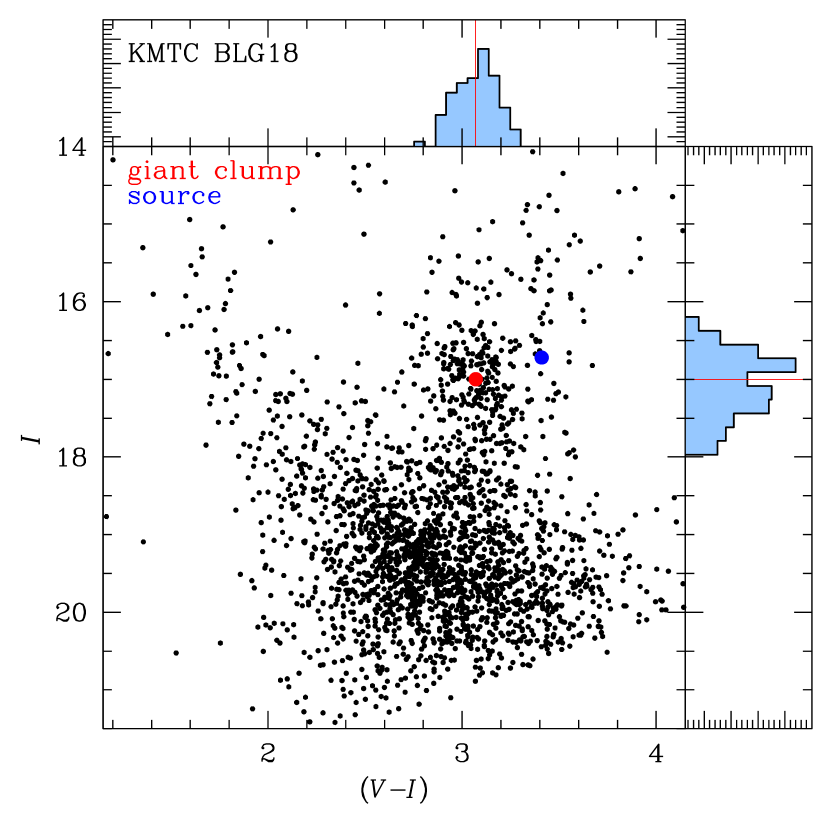
Figure 5: Color-magnitude diagram (CMD) based on KMTC data from a $100^{\prime\prime}$ square centered on KMT-2016-BLG-1107. The source (blue) is more than 0.3 mag redder than the centroid of the red clump (red), and is also more than 0.2 mag brighter. This offset (confirmed also by KMTS data – not shown), leads to a source-radius estimate $\theta_{*}=8.8\pm 0.7\,{\rm mas}$.

We report first the details of the KMTC measurements and then summarize those from KMTS. We find the instrumental $[(V-I),I]$ pyDIA positions of the red clump (see Figure 5),

$$[(V-I),I]_{\rm cl,\rm pyDIA,KMTC}=(2.42,13.97)\pm(0.02,0.04),$$ (8)

and of the source star (by aligning the pyDIA light curves to the best-fitting model,

$$[(V-I),I]_{s,\rm pyDIA,KMTC}=(2.76,13.72)\pm(0.05,0.01).$$ (9)

The offset is therefore $\Delta[(V-I),I]_{\rm KMTC}=(0.34,-0.25)\pm(0.06,0.04)$. Following the same procedure for KMTS, we obtain $[(V-I),I]_{\rm cl,\rm pyDIA,KMTS}=(1.60,14.84)\pm(0.02,0.04)$, $[(V-I),I]_{s,\rm pyDIA,KMTS}=(1.89,14.66)\pm(0.07,0.01)$, and $\Delta[(V-I),I]_{\rm KMTS}=(0.29,-0.18)\pm(0.07,0.04)$. The difference between these two determination has $\chi^{2}=1.8$ for 2 dof, i.e., perfectly consistent. We therefore combine the two measurements to obtain,

$$\Delta[(V-I),I]=(0.32,-0.22)\pm(0.05,0.03).$$ (10)

We adopt $[(V-I),I]_{0,\rm cl}=(1.06,14.36)$ from Bensby et al. (2013) and Nataf et al. (2013) (for $l=2.5$), and so

$$[(V-I),I]_{0,s}=(1.38,14.14)\pm(0.07,0.15).$$ (11)

We note that both of the error bars in Equation (11) are larger than those in Equation (10). For the color, we have added in quadrature 0.05 mag as an estimate of the error in the method, which we derive from the scatter in the difference between spectroscopic and photometric color estimates in Bensby et al. (2013). For the magnitude, we add in quadrature a 0.14 error due to the fractional uncertainty in $f_{s}$ in Table 1.

Using the $VIK$ relation of Bessell & Brett (1988) to convert from $V/I$ to $V/K$ and the color/surface-brightness relation of Kervella et al. (2004), we finally derive,

$$\theta_{*}=8.83\pm 0.73\,\mu{\rm as}.$$ (12)

The main concern regarding systematic errors in this evaluation is that the $V$-band data are too noisy to allow us to independently measure their baseline slope. More precisely, we find that the slope is consistent with the $I$-band slope, but with an error that is twice as large as the value of the $I$-band slope. Because we do not know the origin of this slope, it could in principle be substantially different in the two bands. As a relatively conservative estimate of the impact of this systematic error, we consider two fairly extreme cases: first that the $V$-band baseline is flat, i.e., $dV/dt=0$ and second that it is twice the $I$-band slope, i.e., $dV/dt=0.036\,{\rm mag\,yr^{-1}}$. However, we find that even these changes in assumed slope result in a change in source color of only 0.01 mag, which would result in a change of $\theta_{*}$ that is more than an order of magnitude smaller than the error bar in Equation (12). Hence, this potential source of systematic error has no practical impact. The underlying reason for this is that we evaluate the source flux only using data from a symmetric interval around the peak during which the source is significantly magnified. Because the lightcurve is basically symmetric, while the slope function is anti-symmetric, we expect very little effect. Indeed, it is only because the data sampling is higher on the falling wing of the light curve (because of longer visibility during each night) that there is any effect at all.

Finally, we estimate $\theta_{\rm E}$ and $\mu_{\rm rel}$ for the two solutions.

$$\theta_{\rm E}=0.148\pm 0.021\,{\rm mas};\qquad\mu_{\rm rel}=2.65\pm 0.38\,{\rm mas}\,{\rm yr}^{-1};\qquad(s<1),$$ (13)

$$\theta_{\rm E}=0.048\pm 0.007\,{\rm mas};\qquad\mu_{\rm rel}=0.85\pm 0.13\,{\rm mas}\,{\rm yr}^{-1};\qquad(s>1).$$ (14)

Because of the low values of $\mu_{\rm rel}$ for both solutions, resolution of this degeneracy will require the advent of adaptive optics on next generation (“30m”) telescopes. To evaluate these prospects, we begin by recalling the experience of Batista et al. (2015), who separately resolved the roughly equally-bright source and lens for OGLE-2005-BLG-169 in $H$-band ($1.65\,\mu$m) using the 10m Keck telescope, at a time when these were separated by $60\,{\rm mas}$, i.e., about 1.5 FWHM. Considering that the source is a red giant in the present case, and therefore likely to be 100-1000 times brighter than the lens, we expect that the minimum separation is likely 1/3 larger, i.e., 2.0 FWHM. For the European Extremely Large Telescope 39m telescope in $J$ band (the most optimistic case), this would imply a minimum separation of 14 mas. For an estimated E-ELT AO first light of 2028, this requirement would be satisfied by more than a factor 2 for the $(s<1)$ solution, although it would be only marginally satisfied for the $(s>1)$ solution. Therefore, there are reasonable prospects for resolving this degeneracy at AO first light.

5 Bayesian Analysis

Because the planet-host mass ratio $q$ differs by almost a decade between two solutions that are not distinguishable based on current data, we cannot give even a relatively precise estimate of the planet mass based on a Bayesian analysis. Moreover, if future AO observations (Section 4) do distinguish between the two solutions, there would be no need for a Bayesian analysis because the host mass and distance will be much better constrained by the measurements of $\theta_{\rm E}$ and of the host flux that derive from those observations. Nevertheless, for completeness we carry out a Bayesian analysis to estimate the host mass and distance for each of the two degenerate solutions. We employ the same procedures and Galactic model as did Jung et al. (2018).

The results are illustrated in Figure 6 and summarized in Table 2. For both solutions, the small values of the Einstein radius (Equations (13) and (14)) strongly favor low-mass lenses, while the low proper motions favor Galactic-bulge lenses. In both cases, the effect is substantially stronger for the $s>1$ solution. Also note that even for the close solution, the planet’s projected separation from its host is relatively large for its mass, $a_{\perp}/M\sim 3.9\,{\rm AU}/M_{\odot}$. This would be outside the snowline for a conventional scaling, $a_{\rm snow}=2.7\,(M/M_{\odot})\,{\rm AU}$.

According to Figure 6, there is a roughly 40% probability that the lens will be below the hydrogen burning limit (and hence, likely invisible) even if the $s<1$ solution is correct. This means that if future AO observations fail to detect the host, then we will not be able to determine whether the close or wide solution is correct: all we will know is that the host is a brown dwarf.

6 Discussion: Major/Minor Image Hollywood Degeneracy

6.1 Allowed Range of $s$ for Minor-Image Hollywood Events

When Gould & Gaucherel (1997) derived Equation (1) for the excess magnification $\Delta A\rightarrow 2q/\rho^{2}$ generated by a completely enveloped major-image planetary caustic, they also derived $\Delta A\rightarrow 0$ for a completely enveloped minor-image planetary caustic. Clearly, this formula fails in the present case, for which the $s<1$ solution has a “bump” that looks qualitatively similar to classical major-image Hollywood Cannae “bumps”. This is because the Gould & Gaucherel (1997) analytic result implicitly assumed that the source envelops the entire minor-image caustic structure, including both triangular caustics and the trough that lies between them. In the present case, by contrast, the bump is generated by passing over one of the two triangular caustics, with the source well separated from the other triangular caustic and also from the trough that lies between them.

Hence, the first question to address is: under what conditions can the source completely envelop one triangular caustic and still be well separated from the trough. To address this question, we make use of the analytic results from Han (2006), which are derived in the limit $q\ll 1$. Han (2006) finds that the length of the planetary caustic (along the direction of the binary axis) is

$${\Delta\xi_{c}\over 2}\rightarrow\biggl{(}{27\over 16}\biggr{)}^{1/2}\sqrt{q}s^{3},$$ (15)

while the separation of the center of the caustic from the binary axis is

$$\eta_{c,0}\simeq{\sqrt{q}\over s}[(1+s^{2})^{-1/2}+(1-s^{2})^{1/2}]\rightarrow{\sqrt{q}\over s}(2-s^{2})$$ (16)

Hence, the ratio of the distance of the caustic from the binary axis to its “size” is independent of $q$,

$$R\equiv{\eta_{c,0}\over\Delta\xi_{c}/2}=\biggl{(}{16\over 27}\biggr{)}^{1/2}{2-s^{2}\over s^{4}}$$ (17)

Thus, for $s=(0.4,0.5,0.6,0.7,0.8)$, we have $R=(55,22,10,4.8,2.6)$. Based on this analysis, we conclude that there can be minor-image “Hollywood” type bumps without obvious deviations due to the trough only if $s\lesssim 0.7$.

Another way of stating this result is that a symmetric bump at normalized Einstein-radius position $u_{\rm perturb}\gtrsim 0.7$ can potentially be explained by either a major-image $(s>1)$ or minor-image $(s<1)$ Hollywood solution. On the other hand, for $u_{\rm perturb}\lesssim 0.7$, only major-image Hollywood solutions are viable.

In the present case, $s=0.345$ or $s=2.96$, i.e., $u_{\rm perturb}\simeq 2.6$, we are well into the regime of possible degeneracy between major-image and minor-image Hollywood events.

We note, however, that while $u_{\rm perturb}\gtrsim 0.7$ is a necessary condition, it is not sufficient. It is also necessary that the perturbation occur on the wing (rising or falling) of the light curve rather than near the peak. That is, if the source crosses one triangular caustic near peak, then it will also come close to the other one and will cross the pronounced “dip” in between. These features will be easily recognized in the light curve. In the present case, the anomaly is far into the wing of the light curve and (in the $s<1$ model) the source trajectory runs nearly parallel $(\alpha=\pi+0.11)$ to the binary axis and so essentially never transits the “dip”. See Figure 3. Given less than perfect data, such an extreme geometry is not absolutely required to avoid detection of the dip, but this consideration does generally favor larger $u_{\rm perturb}$ to enable an “effective degeneracy.”

6.2 $\Delta a$: Ratio of $q$ for Major-image to Minor-image Solutions

Gould & Gaucherel (1997) gave an analytic formula (Equation (1)) for the excess magnification $\Delta A$ of Cannae Hollywood events as a function of $q$ and $\rho$. For minor-image Hollywood events there is no such analytic formula, but we can use Equation (1) as a convenient way to normalize $\Delta A$ to make a numerical study of this effect. That is, we define $\Delta a$ as a normalized $\Delta A$,

$$\Delta a\equiv{\rho^{2}\over 2q}\Delta A.$$ (18)

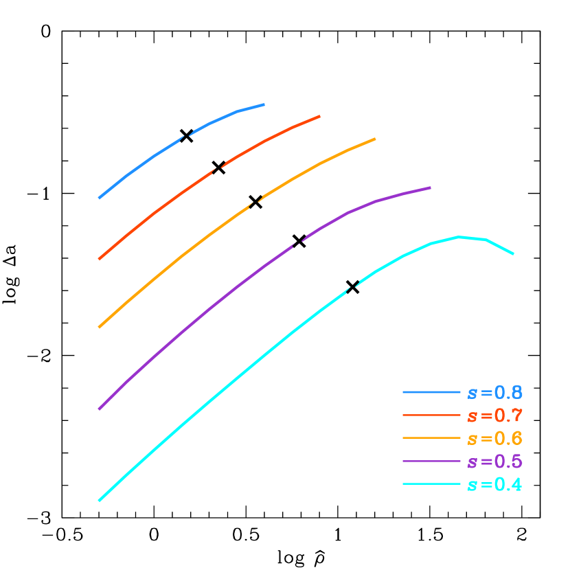
Figure 7: Normalized height of minor-image bump $\Delta a$ (scaled to the analytic result from Gould & Gaucherel 1997 for major-image caustics; see Equation (18)) versus normalized source size $\hat{\rho}$ (scaled to caustic size, see Equation (19)). This diagram is for $q=10^{-3}$, but other values of $q$ are similar. For each curve, the value of $\hat{\rho}$ for which $\rho=\sqrt{q}$ is marked because for major-image caustics, $\rho\gtrsim\sqrt{q}$ implies $\Delta a\rightarrow 1$. The low values of $\Delta a$ generally imply that envelopment of minor-image caustics require much larger $q$ to induce the same size bump compared to major-image caustics.

In Figure 7, we evaluate $\Delta a$ for source stars centered on a minor-image caustic of geometries $(s,q)$, where we fix $q=1\times 10^{-3}$ and consider values of $s=(0.4,0.5,0.6,0.7,0.8)$. In each case, we evaluate $\Delta a$ for values of $\rho$ parametrized by $\hat{\rho}$, i.e., $\rho$ normalized to the caustic size:

$$\hat{\rho}\equiv{\rho\over\Delta\xi_{c}(s,q)/2},$$ (19)

where $\Delta\xi_{c}(s,q)$ is given by Equation (15). In each case, we mark for reference the value of $\hat{\rho}$ for which $\rho=\sqrt{q}$. This value of $\rho$ is relevant for the comparison to major-image Hollywood geometries because for the major-image case, $\rho>\sqrt{q}\Longrightarrow\Delta a\rightarrow 1$.

Figure 7 shows that, particularly for $s\lesssim 0.5$ (i.e., the regime in which degeneracies are likely to be an issue according to the analysis of Section 6.1), $\Delta a$ never rises much above 0.1, i.e., at least an order of magnitude smaller than for the generic major-image case. Hence, according to Equation (18), and assuming similar values of $\rho$, much larger values of $q$ are required to generate a given amplitude of “bump” for minor-image Cannae envelopment compared to major-image Cannae envelopment.

As we have seen for the case of KMT-2016-BLG-1107, the inferred values of $\rho$ are not in fact necessarily the same for the major-image and minor-image solutions. The two solutions must produce the same duration “bump”, but they might achieve this by the caustic traversing different chords through the source, or (as in the present case) by one solution being Cannae and the other von Schlieffen. Nevertheless, Figure 7 indicates an overall tendency toward higher $q$ for the close $(s<1)$ solution, a tendency that is in fact realized in the present case.

6.3 Future Prospects for the Major/Minor Image Hollywood Degeneracy

The short, smooth bump experienced by KMT-2016-BLG-1107 2.5 Einstein crossing times after peak makes it similar in some respects to OGLE-2008-BLG-092 (Poleski et al., 2014), MOA-2012-BLG-006 (Poleski et al., 2017), and MOA-2013-BLG-605 (Sumi et al., 2016). These had $u_{\rm perturb}=4.87$, $u_{\rm perturb}=4.18$, and $u_{\rm perturb}=1.91$ respectively. That is the first two were even further into the wing of the light curve than KMT-2016-BLG-1107, while the last had a comparable value. However, in contrast to KMT-2016-BLG-1107, all three of these earlier events were unambiguously interpreted as having major-image perturbations and, therefore, very wide companions. For MOA-2012-BLG-006 and MOA-2013-BLG-605, this was facilitated by the relatively small source size ($\rho/\sqrt{q}=0.09$ and 0.2, respectively), of the same order as the caustic, which induced some structure on the planetary bump. As noted by Poleski et al. (2014, 2017), events of this type provide a unique probe of very wide separation planets (“Uranus” and “Neptune” analogs), provided of course that they can be unambiguously interpreted as due to very wide (rather than very close) separation companions.

The KMTNet survey is well-suited to detect more events of this type. The radius crossing time of typical giant sources with $\theta_{*}\sim 6\,\mu{\rm as}$, is $t_{*}=13\,{\rm hr}(\mu_{\rm rel}/[4\,{\rm mas}\,{\rm yr}^{-1}])$. Thus, in the $41\,{\rm deg}^{2}$ that are observed at cadences $\Gamma\geq 1\,{\rm hr}^{-1}$ (like BLG18), Hollywood perturbations should be covered very well (weather permitting). Even the additional $44\,{\rm deg}^{2}$ that are observed at $\Gamma\geq 0.4\,{\rm hr}^{-1}$ should yield adequate coverage in many cases. However, more practical experience will be required to determine how often such detections are impacted by degeneracies, and under what conditions these can be resolved.

Table 1: Best-fit solutions

Parameters	$s<1$	$s>1$	1L2S
$\chi^{2}/\rm{dof}$	3894.913/3895	3936.813/3895	4045.87/3895
$t_{0}$ $(\rm{HJD}^{\prime})$	7508.681 $\pm$ 0.068	7509.227 $\pm$ 0.057	7509.034 $\pm$ 0.054
$u_{0}$	0.927 $\pm$ 0.061	0.932 $\pm$ 0.057	0.913 $\pm$ 0.068
$t_{\rm E}$ $(\rm{days})$	20.403 $\pm$ 0.875	20.380 $\pm$ 0.805	20.818 $\pm$ 0.974
$s$	0.345 $\pm$ 0.013	2.965 $\pm$ 0.104	…
$q$ $(10^{-2})$	3.614 $\pm$ 0.544	0.398 $\pm$ 0.059	…
$\alpha$ $(\rm{rad})$	3.132 $\pm$ 0.025	0.441 $\pm$ 0.012	…
$\rho$ $(10^{-2})$	5.955 $\pm$ 0.683	18.411 $\pm$ 2.423	…
$t_{0,2}$ $(\rm{HJD}^{\prime})$	…	…	7557.049 $\pm$ 0.064
$u_{0,2}$	…	…	0.027 $\pm$ 0.013
$\rho_{2}$ $(10^{-2})$	…	…	6.417 $\pm$ 0.877
$q_{F,I}$ $(10^{-3})$	…	…	2.760 $\pm$ 0.306
$f_{s}$	4.065 $\pm$ 0.536	4.201 $\pm$ 0.522	3.977 $\pm$ 0.622
$f_{b}$	-0.439 $\pm$ 0.536	-0.575 $\pm$ 0.522	-0.351 $\pm$ 0.622
$t_{*}$ $(\rm{days})$	1.215 $\pm$ 0.124	3.752 $\pm$ 0.394	…
$t_{\rm eff}$ $(\rm{days})$	18.919 $\pm$ 0.445	18.987 $\pm$ 0.415	…

Table 2: Physical properties

Quantity	$s<1$	$s>1$
$M_{\rm host}$ $[M_{\sun}]$	$0.087_{-0.049}^{+0.092}$	$0.022_{-0.009}^{+0.023}$
$M_{\rm planet}$ $[M_{J}]$	$3.283_{-1.835}^{+3.468}$	$0.090_{-0.037}^{+0.096}$
$D_{\rm L}$ [kpc]	$6.651_{-1.348}^{+0.948}$	$7.481_{-0.708}^{+0.748}$
$a_{\bot}$ [au]	$0.342_{-0.085}^{+0.070}$	$1.065_{-0.189}^{+0.192}$

Figure 3: Caustic geometry of KMT-2016-BLG-1107, close $(s<1)$ solution. The upper panel shows the source trajectory, which grazes the Einstein ring (dashed line) and then fully envelops the tiny triangular caustic, roughly 2.5 Einstein timescales $t_{\rm E}$ later. This Cannae-type Hollywood envelopment is shown in greater detail in the lower-panel zoom, where the source position is shown by circles at the epochs of observations from the three color-coded observatories. During the time that the caustic passes close to the limb, it spends more than half a source-diameter-crossing time inside the source. This should be compared to Figure 4.

Figure 6: Bayesian posteriors for KMT-2016-BLG-1107 for the “close” ($s<1$, left) and “wide” ($s>1$, right) solutions. For both solutions, the small Einstein radius ($\theta_{\rm E}=0.15\,{\rm mas}$ and $\theta_{\rm E}=0.05\,{\rm mas}$) favors a low-mass lens, particularly for the “wide” solution. Similarly, the low proper motion ($\mu_{\rm rel}=2.7\,{\rm mas}\,{\rm yr}^{-1}$ and $\mu_{\rm rel}=0.9\,{\rm mas}\,{\rm yr}^{-1}$) generally favors a bulge lens, and very strongly so for the “wide” solution.

References

- Alard & Lupton (1998) Alard, C. & Lupton, R.H.,1998, ApJ, 503, 325
- Albrow et al. (2009) Albrow, M. D., Horne, K., Bramich, D. M., et al. 2009, MNRAS, 397, 2099
- Batista et al. (2015) Batista, V., Beaulieu, J.-P., Bennett, D.P., et al. 2015, ApJ, 808, 170
- Beaulieu et al. (2006) Beaulieu, J.-P. Bennett, D.P., Fouqué, P. et al. 2006, Nature, 439, 437
- Bensby et al. (2013) Bensby, T. Yee, J.C., Feltzing, S. et al. 2013, A&A, 549A, 147
- Bessell & Brett (1988) Bessell, M.S., & Brett, J.M. 1988, PASP, 100, 1134
- Dominik (1999) Dominik, M. 1999, A&A, 349, 108
- Gaudi (1998) Gaudi, B.S. 1998, ApJ, 506, 533
- Gould (1997) Gould, A. 1997, The Hollywood Strategy for Microlensing Detection of Planets, in Variables Stars and the Astrophysical Returns of the Microlensing Surveys. Eds. R. Ferlet, J.-P. Maillard and B. Raban. Gif-sur-Yvette, France : Editions Frontieres, p.125
- Gould & Gaucherel (1997) Gould, A. & Gaucherel. 1997, ApJ, 477, 580
- Gould & Horne (2013) Gould, A. & Horne, K. 2013, ApJ, 779, L28
- Griest & Safizadeh (1998) Griest, K. & Safizadeh, N. 1998, ApJ, 500, 37
- Han & Gould (1995) Han, C. & Gould, A. 1995, ApJ, 447, 53
- Han (2006) Han, C. 2006, ApJ, 638, 1080
- Henderson et al. (2016) Henderson, C.B., Poleski, R., Penny, M. et al. 2016 PASP, 128, 124401
- Hwang et al. (2018) Hwang, K.-H., Udalski, A., Shvartzvald, Y. et al. 2018, AJ, 155, 20
- Jung et al. (2018) Jung, Y. K., Udalski, A., Gould, A., et al. 2018 AJ, 155, 219
- Kervella et al. (2004) Kervella, P., Thévenin, F., Di Folco, E., & Ségransan, D. 2004, A&A, 426, 297
- Kim et al. (2016) Kim, S.-L., Lee, C.-U., Park, B.-G., et al. 2016, JKAS, 49, 37
- Kim et al. (2018a) Kim, D.-J., Kim, H.-W., Hwang, K.-H., et al., 2018a, AJ, 155, 76
- Kim et al. (2018b) Kim, H.-W., Hwang, K.-H., Kim, D.-J., et al., 2018b, AJ, 155, 186
- Kim et al. (2018c) Kim, H.-W., Hwang, K.-H., Kim, D.-J., et al., 2018c, AAS submitted, arXiv:1804.03352
- Nataf et al. (2013) Nataf, D.M., Gould, A., Fouqué, P. et al. 2013, ApJ, 769, 88
- Paczyński (1986) Paczyński, B. 1986, ApJ, 304, 1
- Poleski et al. (2014) Poleski, R., Skowron, J., Udalski, A., et al. 2014, ApJ, 755, 42
- Poleski et al. (2017) Poleski, R., Udalski, A., Bond, I.A., et al. 2017, A&A, 604A, 103
- Sumi et al. (2016) Sumi, T., Udalski, A., Bennett, D.P., et al. 2016 ApJ, 825, 112
- Udalski et al. (2018) Udalski, A., Ryu, Y.-H., Sajadian, S., et al. 2018, Acta Astron., 68, 1
- Yoo et al. (2004) Yoo, J., DePoy, D.L., Gal-Yam, A. et al. 2004, ApJ, 603, 139