Repeating microlensing events in the OGLE data

Abstract

Microlensing events are usually selected among single-peaked non-repeating light curves in order to avoid confusion with variable stars. However, a microlensing event may exhibit a second microlensing brightening episode when the source or/and the lens is a binary system. A careful analysis of these repeating events provides an independent way to study the statistics of wide binary stars and to detect extrasolar planets. Previous theoretical studies predicted that 0.5 - 2 % of events should repeat due to wide binary lenses. We present a systematic search for such events in about 4000 light curves of microlensing candidates detected by the Optical Gravitational Lensing Experiment (OGLE) towards the Galactic Bulge from 1992 to 2007. The search reveals a total of 19 repeating candidates, with 6 clearly due to a wide binary lens. As a by-product we find that 64 events ($\sim 2\%$ of the total OGLE-III sample) have been miss-classified as microlensing; these miss-classified events are mostly nova or other types of eruptive stars. The number and importance of repeating events will increase considerably when the next-generation wide-field microlensing experiments become fully operational in the future.

1 Introduction

Microlensing events are usually assumed to be single-peaked and constant in the baseline before and after the event. Any additional brightening episode is usually interpreted as an indication of some type of variability other than microlensing. It is a conservative assumption adopted at the beginning of microlensing surveys in the early 1990s. Even now it is still imposed in microlensing searches in very crowded fields heavily contaminated with eruptive variable stars, e.g. towards Magellanic Clouds or M31.

However, microlensing is now well established and many events are routinely discovered in real-time. It is well-known that in principle a small fraction of microlensing events can repeat. By repetition we mean a second brightening episode well after the first one such that the star has (largely) returned to its baseline. A variety of scenarios can cause repetitions, for example, when the lensed source is a binary wide enough for the lens to magnify both components separately, one after another. The binarity of source does not have to be physical, as the lens can sequentially magnify two unrelated stars blended in one seeing disk. Another mechanism that can produce two independent peaks in the light curve is a lens consisting of two gravitationally bound components with large separation magnifying a single source. The lensing of a physical binary by another physical binary can result in diverse light curve shapes, which in some cases may mimic repeating events. This rather complicated scenario is not pursued in this analysis of limited number of candidate events. One can even imagine two independent masses acting as lenses. This is, however, expected to occur with a much smaller probability since the microlensing optical depth for a single event is already low ($\sim 10^{-6}$), and thus we do not study such a scenario in this paper.

Griest & Hu (1992) investigated the effects of the binarity of sources on the properties of light curves produced by a single lens. They concluded that, depending on the adopted population of the binary population and the lens mass function, the cases with double peaks and asymmetric light curves (easily distinguishable from single source events) comprise 1% to 3% of all events.

Di Stefano & Mao (1996) studied the possibility of repeating microlensing due to wide binary lenses and predicted that 0.5-2 per cent of observed microlensing curves should exhibit apparent repetitions. The fraction is lower than that predicted for “ordinary” binary events with smaller separations (Mao & Paczyński 1991). To date, hundreds of ordinary binary microlensing events have been discovered (Alcock et al. 2000; Collinge 2004; Jaroszyński et al. 2004, 2006; Skowron et al. 2007), but only one “repeating” binary event was found (OGLE-2003-BLG-291) and was studied in detail by Jaroszyński et al. (2005).

Thanks to microlensing surveys such as the Optical Gravitational Lensing Experiment (OGLE, Udalski 2003 and Microlensing Observations in Astrophysics (MOA, Yock 1998), several thousand microlensing events have been detected in real-time. Among these, we would expect tens of events caused by wide binaries.

Detection and studies of these events are interesting for two important reasons. First, these events provide an independent way of studying the statistical properties of the binary star population, including the distribution of mass ratios and separations. Since a large fraction of lens population is expected to be composed of low-mass ($\sim 0.3M_{\odot}$) main sequence stars, the detection of the binary companions around these faint stars would be difficult using spectroscopic methods (e.g. Fisher et al. 2005), because of their typically long periods, small accelerations and slow radial velocity variations. The novel aspect of the microlensing method is that we can infer the mass ratios in the time domain simply from the ratio of the timescales in the two brightening episodes (see §5) rather than using spectroscopy (Di Stefano & Mao, 1996). Second, repeating microlensing events can in principle be used to detect planetary companions (Di Stefano & Scalzo, 1999); this would be an extension of the methods used currently by the survey and followup teams for successful detections of extrasolar planets (e.g. Bond et al. 2004; Udalski et al. 2005; Beaulieu et al. 2006; Gould et al. 2006; Gaudi et al. 2008).

In this work we present the results of a systematic search for repeating events in the available data on all microlensing candidates detected by the OGLE team. The paper is organised as follows. Sections 2 and 3 describe observational data and our search procedure. In Section 4 we focus on different microlensing models and algorithms to fit the light curves of repeating candidates. The major results of our search are presented in Section 5, and we summarise and further discuss our results in Section 6.

2 Observational data

In this study we use data acquired by the first, second and third phases of OGLE. The readers are referred to Udalski (2003) for more technical details about these phases of the project. We gather all the microlensing events detected by the OGLE Early Warning System (EWS), by OGLE-II (1998-2000, Udalski et al. 1994) and by OGLE-III (2001-2007, Udalski 2003). We also include events found independently by Woźniak et al. (2001) in the OGLE-II 1997-1999 data and by Wyrzykowski (2005) and Wyrzykowski et al. (2006) in the OGLE-III 2001-2005 data. In total there are 4120 unique microlensing candidate events. The systematic checking of a possible later (or an overlooked earlier) episode of variability of sources belonging to EWS catalogs is not routinely done, and this task is undertaken here. Notice that events with closely separated peaks may be removed from the candidate list, and thus we focus on “repeating” events where the star has (largely) returned to its baseline between the episodes since such events will not be rejected by the EWS.

For each event, we check if any additional observational data are available in the OGLE-I (1992-1995), OGLE-II (1996-2000) and OGLE-III (2001-2007) databases. The maximum available time span is therefore 15 years. 152 microlensing events were observed continuously during all three phases of the OGLE project (15 years). About 1200 events were observed continuously for 10 years and about 2300 for 5 years.

3 Searching for repeating events

For each of the 4120 light curves, we search for the presence of two or more magnification episodes in the whole time span by visual inspection and with a semi-automated algorithm. We discuss these two approaches in turn.

3.1 Visual inspection

The main criterion used in this subjective analysis is the presence of a significant bump before or after the main brightening episode. We look for events, where the brightenings are separated by a return of the light curve to the baseline. Our systematic inspection of all the 4120 light curves has revealed 13 candidates of repeating events.

In addition, a small number of objects have been found among the microlensing candidates being other types of brightenings. They are present only in among events listed by the EWS because of the nature of the EWS detection algorithm, which detects significant and continuous brightening, but does not perform any microlensing model fitting. The main contamination is from nova-like outbursts and from other variables, mostly eruptive stars. The long time span allows a better classification of the events, e.g. by identifying later outbursts or another period in oscillations. In addition most of these stars exhibit some asymmetry in their brightening episodes.

The largest and most uniform sample is from the EWS in the OGLE-III phase (until September 2007). Out of 3159 microlensing candidates in this sample, 64 ($\sim 2\%$) turn out to be intrinsically variable stars; 24 of these show a behaviour similar to dwarf novae stars with multiple, short-time outbursts. Furthermore, 52 events ($\sim 1.6\%$) have duplicate entries since they were “discovered” twice in overlapping adjacent fields.

3.2 Semi-automated search algorithm

The main goal for developing an automated algorithm is to identify repeating events in which the second magnification episode is considerably smaller than the first one, as such configuration would be easier to miss visually. Because of the contamination by variable stars and caustic crossing events we were only able to construct a semi-automated algorithm, which still required some human supervision.

In the first step we detect the main microlensing episode and fit it with the Paczyński (1986) model. The portion of this model light curve which is above $3\sigma$ level from the baseline defines the duration of the brightening episode, and the corresponding data points are removed from the light curve. The fit of the Paczyński model does not have to be perfect, since it only serves to mark the brightening episode, and our experience shows that the same algorithm can also be successfully applied to binary lensing events.

A constant light curve model and the Paczyński model are then fit to the remaining data, yielding two $\chi^{2}$’s: $\chi^{2}_{\rm 2nd,const}$, and $\chi^{2}_{\rm 2nd,Pac}$. If a repeating event is present, $\chi^{2}_{\rm 2nd,Pac}$ is expected to be substantially smaller than $\chi^{2}_{\rm 2nd,const}$.

To ensure the second fit is reliable, we calculate the number of data points in the second magnification episode, $n_{\rm 2nd}$, and reject all events with $n_{\rm 2nd}<3$ or $n_{\rm 2nd}>N/2$, where $N$ is the total number of data points. We then construct the following statistic:

$$s=\frac{|\chi^{2}_{\rm 2nd,Pac}-\chi^{2}_{\rm 2nd,const}|}{\chi^{2}_{\rm 2nd,Pac}},$$ (1)

and choose events with $s>0.2$. This ad hoc criterion typically corresponds to a fit improvement in $\Delta\chi^{2}$ of several tens, which is high enough to avoid false identifications (cf. §5.1.2). On the other hand all 13 events found by visual inspection are recovered.

A total of 193 events have passed the described criteria. All of them have been examined visually giving 6 new candidates, and bringing the total number of candidates for repeating events to 19 (see Table 1). 6 new candidates were overlooked during the visual inspection due to their small amplitude of the secondary peak.

3 out of 19 of our candidates were found in previous studies: the connection between two EWS events OGLE-1999-BUL-42 and OGLE-2003-BLG-220 was found by Klimentowski (2005); OGLE174828.55-221639.9 was found by Wyrzykowski (2005) and OGLE-2003-BLG-291 was described in detail by Jaroszyński et al. (2005).

4 Modeling

All 19 events were fitted with three different models: binary source, binary lens and approximate wide binary lens models.

We model a binary lens following Skowron et al. (2007). In total there are seven parameters. The two point lenses are described by the mass ratio ($q$) and separation ($d$) in units of the Einstein radius ($r_{E}$). The microlensing geometry is described by the impact parameter ($b$), the angle between the source trajectory and the projected binary axis ($\beta$ in degrees), Einstein-radius crossing time ($t_{E}$ in days), the time of the closest approach to the center of mass of the binary ($t_{0}$), and the fraction of light contributed to the total blended flux by the lensed source, $f$ ($f=1$ indicates no blending). The event baseline magnitude ($I_{0}$) is measured separately. A point-like source is assumed in the fitting. In some cases in order to better fit the observational data we further introduce the parallax motion of the Earth (with a parallax scale $\pi_{E}$, defined as $1{\rm a.u.}/\tilde{r}_{\rm E}$, where $\tilde{r}_{\rm E}$ is the radius of the Einstein ring projected into the observer’s plane) and/or the rotation of the binary lens assuming circular face on orbits (with an angular velocity of $\dot{\beta}$ in units of deg yr^-1).

The first stage of searching for the best-fit models was, however, done on a grid more appropriate for uncovering repeating events. The grid covers a wide range for 6 parameters: the mass ratio, binary separation, minimum distances to the source trajectory from the first and second mass and their corresponding times of minimum approach. The starting values for the approach times are estimated from the visual inspection of the light curve. For fixed distances from the two masses, two source trajectories are possible depending on whether the source trajectory intercepts the binary lens axis or not. Each parameter is sampled with about 15-20 intervals. These initial searching parameters are then transformed to the “standard” model parameters mentioned above and the $\chi^{2}$ is calculated. A few hundred models with low $\chi^{2}$’s from the grid are taken as initial guess parameters and fed into a minimisation procedure based on the Powell’s method (Press et al. 1992).

We also fit a simple static binary source model to each event. In this model, the light curve is a sum of two standard single microlensing events with two impact parameters ($b_{1}$ and $b_{2}$), two parameters for the times of maximum magnification ($t_{01}$ and $t_{02}$), fractions of light contributed to the total light by the two sources ($f_{1}$, and $f_{2}$, $f_{1}+f_{2}\leq 1$), baseline magnitude ($I_{0}$) and Einstein radius crossing time ($t_{E}$). To ensure the resulting models are comparable with the binary lens models a similar minimisation strategy is used with the same grid sizes and optimisation routines as those for the binary lens model. Notice that the binary source model was fit only to non-caustic crossing events since the binary source models cannot reproduce the sharp gradient features in caustic-crossing events. In addition, we apply an approximate wide binary model following the concept of Di Stefano & Mao (1996). In this model, the binary lens acts as two independent single lenses. If the two individual magnifications are given as $\mu_{1}$ and $\mu_{2}$, then the resulting magnification is approximated as $\mu\approx\mu_{1}+\mu_{2}-1$. The fitting is done on a grid similar to that for the full binary lens model. In practice it is important to fit both bumps simultaneously to ensure the same constraints on the blending (and other) parameters. Due to the degeneracies in the blending model (Woźniak & Paczyński 1997), fitting each peak independently gives uncertain estimation of fluxes and timescales.

Notice that the two (smooth) peaks produced by a wide binary lens correspond to the source approaches to the diamond shaped caustics, not to the lens components. Since both caustics lie between the masses, fitting the simplified model systematically under-estimates the binary separation and may give incorrect trajectory direction. However, since we are primarily interested in the mass ratio of the binary which are given by the ratio of the squares of the timescales of two magnification peaks (Di Stefano & Mao 1996), this is not a significant limitation (see §5 and Fig. 2).

5 Results

Table 1: Candidates for repeating microlensing events.

Event OGLE-	$(f_{1}/f_{2})_{\rm bs}$	$q_{\rm bl}$	$q_{\rm approx}$	Type
1999-BUL-42	model not found			cc bl?
1999-BUL-45	0.189	0.203	0.270	bl/bs
2000-BUL-42	0.260	0.339	0.400	bl
2002-BLG-018	0.280	0.395	0.443	bs/bl
2002-BLG-045	0.045	0.008	0.011	bl
2002-BLG-128	–	0.611	–	cc bl
2003-BLG-063	0.539	0.203	0.428	bl
2003-BLG-067†	0.817	0.788	0.844	bs/bl
2003-BLG-126	0.292	0.604	0.918	bl
2003-BLG-291	–	0.617	–	cc bl
2003-BLG-297	0.075	0.147	0.121	bl/bs
2004-BLG-075	0.707	0.587	0.664	bl/bs
2004-BLG-328	0.150	0.056	0.054	bs
2004-BLG-440	0.927	0.622	0.906	bl
2004-BLG-591	0.548	0.507	0.431	bl
2006-BLG-038	–	0.569	–	cc bl
2006-BLG-460	0.388	0.267	0.285	bl
175257.97-300626.3	–	0.195	–	cc bl
174828.55-221639.9	–	0.158	–	cc bl

Light ratio from binary source model and mass ratios from full ($q_{\rm bl}$) and approximate ($q_{\rm approx}$) binary lens models are shown. The last column indicates whether the binary lens (“bl”) or binary source (“bs”) model is better. “bl/bs” stands for comparable binary lens and binary source models. Events with clear caustic crossing features (“cc bl”) admit only the full binary lens model. ${\dagger}$ Modelling for this event indicates it did not fully return to the baseline between the peaks (see the light curve in the Appendix). Nevertheless, we include this event because of the lack of sufficient data points around the “saddle point” between the peaks.

Table 1 lists all 19 candidates for repeating events. It shows also the mass ratios in the full and approximate wide binary lens models and the light ratio from the binary source model. The last column in the Table indicates the nature of each event as concluded from a comparison of the best $\chi^{2}$ values of the binary lens and binary source fits. The two models are regarded as comparable when their $\chi^{2}$ values differ by less than $10$. In our terminology, “bl” stands for binary lens, “bs” for binary source and “cc bl” indicates that the caustic crossing features are clearly visible in the light curve for which, therefore, only the full binary lens model is fit. The parameters of the best-fit binary lens and binary source models are listed respectively in Tables 2 and 3. The light curves of all the events are shown in the Appendix.

The smooth (non-caustic-crossing) light curves with two peaks quite often have concurrent, similar quality fits based on binary source and binary lens models. This degeneracy is also known for events with much shorter duration, when the peaks partially overlap (Jaroszyński et al. 2004, 2006; Skowron et al. 2007; Collinge 2004). Since binary lenses offer a much larger variety of possible light curve shapes, their fits are usually formally better.

Clear caustic crossing features can be seen in the light curves of about 30 per cent of our candidates. This fraction is an order of magnitude higher than that in the whole sample of microlensing events – in the uniform sample of 3159 candidates from the EWS from OGLE-III, 73 events ($\sim 2.4\%$) show clear caustic crossing features in their light curves. Our simulations (section 5.1) show that assuming all our candidate events were caused by wide binary lenses we should expect that approximately 10-30 per cent should exhibit caustic crossing features (the fraction increases as the mass ratio decreases). The high fraction of caustic crossing events in our sample of repeating events suggests that the binary lens scenario is favoured for the majority of our candidates.

The number of binary source events in our sample appears to be too low when compared with predictions of Griest & Hu (1992), Han & Jeong (1998), Dominik (1998). Even if all ambiguous cases were classified as binary source events, we would get probability of only 0.15% for their occurrence, much lower than the percentage from these studies. Our sample, however, includes only the events with well separated peaks, while the other authors include close binary sources, which have the highest probability of producing an event distinguishable from ordinary microlensing light curve.

Table 2: Parameters of the best-fit binary lens models.

Event	$\chi^{2}$/DOF	$q$	$d$	$\beta$	$b$	$t_{0}$	$t_{E}$	$f$	$I_{0}$
1999-BUL-42	=2003-BLG-220, model not found, see text
1999-BUL-45	645.4/405	0.203	4.104	18.00	0.47	1401.6	30.2	1.00	17.75
2000-BUL-42	8852.0/697	0.339	5.308	22.40	1.09	2096.7	99.0	0.37	13.58
2002-BLG-018	142.9/111	0.395	6.572	-1.30	0.44	2510.3	34.6	0.91	18.06
2002-BLG-045	3222.7/633	0.008	3.958	183.49	-0.22	2360.8	26.4	0.97	18.76
2002-BLG-128	2218.6/810	0.611	1.908	173.84	0.22	2463.2	59.5	0.12	17.74
2003-BLG-063	1105.4/317	0.203	3.154	25.76	1.39	2869.3	54.5	0.78	16.13
2003-BLG-067	1236.4/323	0.788	3.636	0.60	0.47	2942.4	88.6	0.62	16.45
2003-BLG-126	1027.9/295	0.604	2.808	-34.80	-0.92	2804.2	22.8	1.00	15.66
2003-BLG-291†	912.8/251	0.617	3.041	184.70	0.50	2925.8	43.5	0.38	17.45
2003-BLG-297	984.6/297	0.147	2.912	179.33	0.51	2963.3	75.5	1.00	17.31
2004-BLG-075	555.5/203	0.587	4.456	-11.09	-0.19	3097.8	9.7	1.00	18.82
2004-BLG-328	2782.3/545	0.056	3.399	175.70	0.20	3181.5	25.3	0.20	18.45
2004-BLG-440	2220.0/527	0.622	4.499	158.66	0.65	3183.1	8.6	0.36	16.34
2004-BLG-591	2478.3/672	0.507	2.874	4.69	0.26	3426.9	81.4	0.29	18.48
2006-BLG-038	3556.7/744	0.569	3.138	206.47	-0.68	3809.4	12.7	1.00	16.44
2006-BLG-460	2418.9/862	0.267	3.354	178.85	0.11	3982.7	20.0	0.69	19.10
175257.97-300626.3‡	4845.1/932	0.195	3.268	-171.58	-0.37	2547.4	102.9	0.35	18.19
174828.55-221639.9§	406.2/192	0.158	2.431	172.48	-0.06	2827.7	155.2	0.31	18.93

The columns are respectively, the name of the OGLE event, $\chi^{2}$/number of degree of freedom (DOF), mass ratio $q$, binary separation $d$ (in units of the Einstein radius), direction of the source trajectory with respect to the binary axis $\beta$ (in degrees), impact parameter $b$, time of the closest approach to the center of mass $t_{0}$ (Julian date shifted by 2450000), Einstein radius crossing time $t_{E}$ (in days), blending parameter $f=F_{s}/F_{0}$ and I-band brightness of the baseline $I_{0}$.

${\dagger}$ The model for the event 2003-BLG-297 is taken from Jaroszyński et al. (2005) which includes binary rotation. ${\ddagger}$ model with parallax motion, $\pi_{E}=0.279$. $\S$ model with binary axis rotation, $\dot{\beta}=0.032^{\circ}/{\rm day}$.

Table 3: Parameters of the best-fit binary source models.

Event	$\chi^{2}$/DOF	$b_{1}$	$b_{2}$	$t_{01}$	$t_{02}$	$t_{E}$	$f_{1}$	$f_{2}$	$I_{0}$
1999-BUL-42	—
1999-BUL-45	646.4/405	0.450	0.546	1310.64	1420.33	35.8	0.109	0.576	17.75
2000-BUL-42	8922.8/697	0.539	2.386	1748.74	2221.12	66.5	0.207	0.793	13.58
2002-BLG-018	142.2/111	0.473	0.428	2350.71	2573.40	31.9	0.218	0.778	18.06
2002-BLG-045	3269.6/633	0.220	0.002	2359.97	2457.28	25.8	0.957	0.043	18.76
2002-BLG-128	—
2003-BLG-063	1198.6/317	0.586	1.675	2748.84	2891.19	29.2	0.350	0.650	16.13
2003-BLG-067	1228.8/323	0.420	0.451	2771.86	3077.76	83.9	0.273	0.334	16.45
2003-BLG-126	1221.7/295	0.136	1.120	2774.55	2831.55	15.4	0.774	0.226	15.66
2003-BLG-291	—
2003-BLG-297	989.4/297	0.437	0.295	2934.13	3143.78	78.6	0.682	0.051	17.31
2004-BLG-075	560.8/203	0.304	0.448	3072.38	3112.70	9.6	0.414	0.586	18.82
2004-BLG-328	2710.3/545	0.240	0.004	3177.38	3255.48	26.1	0.204	0.031	18.45
2004-BLG-440	2237.1/527	1.897	0.624	3169.26	3204.09	5.3	0.515	0.477	16.34
2004-BLG-591	2489.5/672	0.046	0.200	3289.05	3499.46	106.8	0.063	0.115	18.48
2006-BLG-038	—
2006-BLG-460	2455.2/862	0.099	0.054	3969.47	4030.86	22.9	0.470	0.183	19.10
175257.97-300626.3	—
174828.55-221639.9	—

The columns show the name of the OGLE event, $\chi^{2}$/the number of DOF, impact parameters $b_{1}$ and $b_{2}$ for two source stars, times of closest approach to both components $t_{01}$ and $t_{02}$, Einstein radius crossing time $t_{E}$, blending parameters $f_{1}=F_{s1}/(F_{s1}+F_{s2}+F_{b})$ and $f_{2}=F_{s2}/(F_{s1}+F_{s2}+F_{b})$, and I-band brightness of the baseline $I_{0}$. $F_{s1}$ and $F_{s2}$ are the fluxes from the two sources, and $F_{b}$ is the flux from any other unrelated star(s) within the seeing disc (blend).

One practical issue one needs to know for future search for repeating events is how long an observer has to wait for the secondary episode to occur. This is illustrated in Figure 1 showing the time between the two peaks vs. the event timescale. As predicted in Di Stefano & Mao (1996) this time is of the order of a few (from 2 to 6) Einstein-radius crossing times. For the repeating events described here this is between 32 to 472 days with a median of 142 days.

Figure 1: Time between two peaks in repeating events versus the Einstein radius crossing time, $t_{E}$.

Since the approximate binary model gives a quick way to estimate the binary mass ratios (see §4), it is important to check its accuracy. Figure 2 compares the mass ratios in the full and approximate binary lens models where both fits are available. A strong correlation is clearly visible (with an RMS difference of about 36%), indicating that the simplified model can indeed be used to estimate the mass ratio in repeating events due to wide binary lenses.

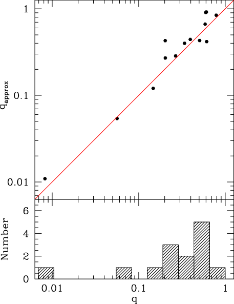
Figure 2: Correlation between the mass ratios obtained in the full ($q$) and approximate ($q_{\rm approx}$) binary lens models (upper panel) and the observed histogram of mass ratios derived in the full binary lens model (lower panel).

5.1 Distribution of binary lens mass ratios

The histogram in the bottom panel of Fig. 2 shows the distribution of the mass ratio in the wide binary lens models. It shows a peak around $q\sim 0.5$ and a decrease for small values of $q$. The decrease is, however, likely due to a larger incompleteness at small $q$ in the observations. Thus to uncover the true distribution of mass ratios, we have to correct the histogram in Fig. 2 for the detection efficiency.

5.1.1 Simulations of detection efficiency for wide binary lenses

A rigorous detection efficiency analysis at the pixel level involves many factors and is beyond the scope of the paper. However, since our sample is small and Poisson errors are large (see Fig. 3), a first-order approach at the catalog level is sufficient to account for the primary selection effects for wide binaries with different mass ratios.

We perform simulations of repeating events due to wide-separation lenses with the mass ratio ranging from $10^{-3}$ to 1 at 25 uniform, logarithmically-spaced intervals. Depending on the mass ratio, about $10^{4}-10^{5}$ binary lensing events are generated. An automated algorithm for identifying the fraction of repeating events observed in the sample is then used (see §5.1.2).

To create a synthetic microlensing event, we first generate a physical model of a binary lens and source trajectory and then based on the physical model, a light curve with sampling rates similar to those of OGLE is simulated. To generate a binary microlensing model the following steps are performed:

1. For a given mass ratio, a binary separation is drawn from the range 1 to 36 Einstein radii using a uniform distribution in logarithm. Our simulations show that the detection efficiency falls to zero outside this range. For lenses of masses $M\in[0.1,1]~{}M_{\odot}$ placed in the Galactic disk and sources in the bulge, the above range corresponds roughly to physical separations of $1$ – $100~{}\mathrm{AU}$.

2. To ensure at least one magnification episode, we set the source trajectory to pass the heavier lens at an impact parameter from 0 to 1 Einstein radius.

3. The trajectory angle is set randomly from 0 to 360 degrees.

4. The time of the closest approach to the heavier mass is chosen from a uniform distribution to lie within the whole observing time.

5. The Einstein-radius crossing time is drawn from an approximate distribution that matches that of the observed OGLE lenses: a log-normal distribution centered on $t_{E}=26$ days with a standard deviation of 0.3.

After the physical model is chosen using the procedure described above, the magnification as a function of time can be easily found. However, to mimic an observed light curve, several further steps are necessary.

1. The baseline magnitude is chosen randomly from the luminosity function of one of the OGLE fields (BLG104.6).

2. The value of the blending parameter is chosen at random between 0 and unity. The small sample of binary lens models (Jaroszyński et al. 2004) supports such a choice of the blending parameter distribution. The values of the baseline flux and blending parameter combined with the theoretical lens model yield a perfect light curve without errors.

3. To account for observational gaps in the light curve, the epochs of observations are chosen so as to match either BUL_SC34.I.36546 in OGLE-II or BLG104.6.I.7723 in OGLE-III. They have been chosen as a reference for epochs and observational errors (to be used in eq. 2) as their light curves span from 1998 to 2007 during which all our repeating events candidates have been found.

4. Each measurement has an observational error $\Delta I$ from the rescaled values for a reference star $\Delta I_{\rm ref}$ using the empirical formula from Wyrzykowski (2005):

   $$\Delta I=\Delta\,I_{\rm ref}10^{0.33875(I-I_{\rm ref})}$$ (2)

   where $I$ is the model magnitude, $I_{\rm ref}$ is the magnitude and $\Delta I_{\rm ref}$ is the error bar for the reference star at the epoch.

5. Gaussian errors are added to the light curve. In this step, we take into account the fact that OGLE errors are slightly underestimated: for every simulated data point, a Gaussian standard deviation is derived based on its error bar value $\Delta I$ in eq. (2) using

   $$\sigma=\sqrt{(1.38\Delta I)^{2}+0.0052^{2}}.$$ (3)

   This rescaling has been obtained following the method of Wyrzykowski et al. (2008) by comparing the rms of a set of constant stars to their mean error bars returned by the photometry pipeline.

5.1.2 Efficiency-corrected statistics of binary mass ratios

To calculate the detection efficiency of repeating events for a given mass ratio, all the light curves of synthetic events must be classified. To accomplish this, we fit a standard Paczyński model to all the light curves and compare the resulting $\chi^{2}$ with a constant line fit. We have also applied the same procedure to check if a Paczyński model fit to a constant luminosity light curve (with Gaussian errors) can improve the fit. Our experiment shows that the typical improvement for $\sim 10^{3}$ d.o.f. is $\Delta\chi^{2}\approx 15$ and exceeds 55 in $\sim 1\%$ of cases. When investigating the synthetic light curves, we require a $\Delta\chi^{2}>55$ improvement of the Paczyński model over the constant line model to treat the event as a microlensing candidate. (Notice that while each curve is simulated using microlensing, the gaps between the seasons and/or sampling rate may prevent it from being “discovered”.)

We then use our automated algorithm (see §3.2) to identify repeating events in our sample. The relative detection efficiency is then defined as the ratio of repeating events ($N_{\rm rep}$) found in the sample of all identified microlensing events ($N_{\rm events}$). Figure 3 shows the efficiency with respect to mass ratio ($q$). It can be approximated by the formula $N_{\mathrm{rep}}/N_{\mathrm{event}}\approx 0.021q^{0.687}$.

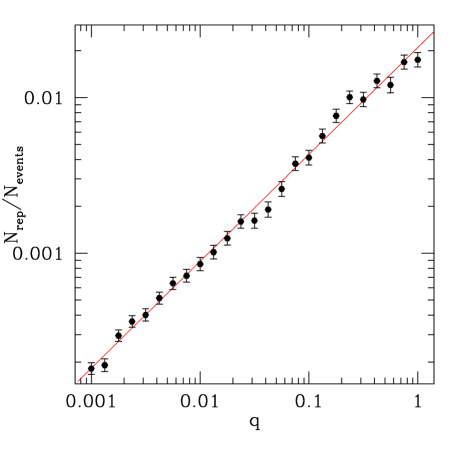
Figure 3: Relative detection efficiency, defined as the ratio of the number of detected “repeating” events and the total number of detected microlensing events, as a function of the mass ratio $q$. Error-bars denote Poisson noise based on population of simulated sample. The solid line is an empirical fit of $N_{\mathrm{rep}}/N_{\mathrm{event}}\approx 0.021q^{0.687}$.

Fig. 4 shows likely underlying distribution of binary mass ratios obtained by convolution of observed mass ratios (Fig. 2) and their detection efficiency (Fig. 3). For mass ratios between $0.07\la q\la 1$, the distribution is consistent with a uniform distribution in the logarithm of mass ratio with Poisson errors, in agreement with earlier results of Trimble (1990). Although we have one event (OGLE-2002-BLG-045) for the smallest mass ratio bin, because of the low detection efficiency for such events, the inferred relative number is quite high, but the error bar is large. Nevertheless, it may indicate the presence of a different population of binary (planetary) systems with extreme mass ratios.

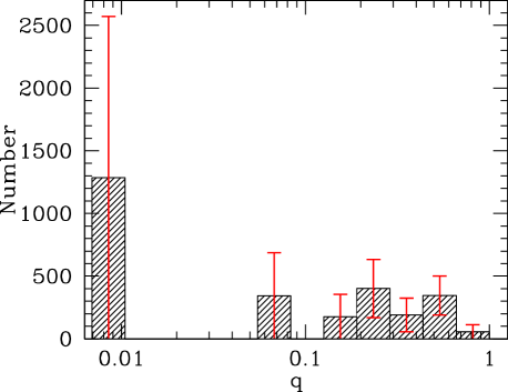
Figure 4: Distribution of binary mass ratios after correcting for detection efficiency. Error bars are from the Poisson noise. The left-most bin at $q=0.01$ contains only one event.

Assuming a uniform distribution of binary lenses in $\log\,q$ and $\log\,d$, we can calculate the averaged efficiency of the detection for $q\in[0.1,1]$ and $d\in[1,36]r_{E}$, obtaining $<N_{\mathrm{rep}}/N_{\mathrm{events}}>=0.0105$. Notice that we have excluded the brown dwarf and planetary binary companions (with mass ratios between $q\in[0.001,0.1]$ since there is only one such planetary candidate. If all the events were caused by binary lenses with parameters from this range, one would expect $4120\times 0.0105\approx 43$ detections of repeating events. Since twelve repeating events are unambiguously classified as binary lens cases, this suggests that at least 28% of all lenses are binary systems within the specified range in the mass ratio and separation. Binary stars roughly follows a uniform distribution per decade of separation between $10^{11}$ cm to $10^{17}$ cm (Abt 1983; Mao & Paczyński 1991), thus we expect a fraction of $\log(36/1)/6=26\%$ within $d\in[1,36]r_{E}$, in good agreement with the 28% we estimated above if all the lenses are in binary systems. However, earlier studies indicate that about 50% of solar-type stars are in binary stars, while for M stars this fraction may be even lower (Duquennoy & Mayor 1991; Fisher & Marcy 1992; Reid & Gizis 1997; Lada 2006 and references therein), thus we would expect a factor of $\sim 2$ smaller number of repeating events due to binary lenses. There are several possiblities to explain the “discrepancy”. 1) It may simply be due to small number Poisson fluctuation. 2) The binary fraction is under-estimated in spectroscopic surveys. 3) The distributions of the separation and mass ratio may differ from being uniform per decade as we assumed (our data are consistent with this assumption within the small number statistics.) 4) Some of the “repeating” events are actually not due to binary lenses. In the future, with a much larger number of repeating events and denser time samplings (e.g., with OGLE-IV), we will be in a better position to test these different possibilities.

5.2 Comments on two individual events

In this section, we study two particularly interesting “repeating” microlensing events. OGLE-1999-BUL-42/OGLE-2003-BLG-220, and OGLE-2002-BLG-045 in more detail.

5.2.1 OGLE-1999-BUL-42/OGLE-2003-BLG-220

For this event, we were not able to find any satisfactory model. This interesting case requires closer scrutiny. The light curve of the event in 1999 resembles a caustic crossing binary lens, but because of the lack of sharp features it can also be explained by a binary source model. However, a static binary source model turns out to be insufficient. The secondary bump from 2003 shows nearly no binarity features except one outlying data point and a slight asymmetry.

The timescales of both magnification episodes are of the order of 20 days and the separation between them is very long, about 1400 days. This indicates it is unlikely that both bumps were produced by a very wide binary lens, because such lenses have tiny caustics and as such they cannot explain the features in the light curve from 1999. One possible scenario for the repeatability is that the source was lensed by two unrelated lenses or two sources were lensed by one binary lens; the event may also be due to a variable star rather than microlensing.

We have attempted to gain some additional insights using information available from the OGLE photometry pipeline using the Difference Image Analysis (DIA) (Woźniak, 2000). In this method all variable sources are detected on the subtracted image and for each variable the centroid of the subtraction residuals indicates the real position of the variable star. Because of blending this position may not be aligned with the position of the baseline star on the template image. In the OGLE database (A. Udalski, private communication) we checked the positions of the residuals with respect to the template positions around the 1999 and 2003 peaks. Because of sparse sampling there are only a few high signal-to-noise measurements in the 2003 peak, however we can still confirm that the position of the lensed source is consistent with the centre of the blend. This does not necessarily mean there was no blending, but simply that the source happens to be located near the centre of the blended object. On the other hand, the 1999 peak had a much better coverage and the detected astrometric signal is firm, showing a clear displacement of the residuals in respect to the blended position by about 150-200 mas. This result indicates that it is unlikely the 1999 and 2003 events were caused by the same lens, unless it moves very fast ($\sim 40\,{\rm mas/yr}$) and/or is a very close object. The remaining (microlensing) hypothesis is that it is a pair of completely unrelated events occurring on two different sources. Further studies, including high resolution imaging (e.g. with the Hubble Space Telescope), would either confirm or reject this scenario.

5.2.2 OGLE-2002-BLG-045

The second brightening of this event was much shorter than the first one and the binary lens model gives a low mass ratio of $q=0.008$ (the approximate binary lens model gives $q=0.011$). For a typical lens mass of about $0.3M_{\odot}$, this would imply a planet mass of a few Jupiter masses. Unfortunately, sparse sampling of both peaks prevent us from concluding convincingly the planetary nature of the lens. Nevertheless this demonstrates repeating events may be a potentially exciting channel of detecting planets in repeating events (e.g., Di Stefano & Scalzo 1999).

5.3 Contaminants to the OGLE Early Warning System

As a by-product of our search, we identified a number of non-microlensing events in the database. In total we found 64 mis-classified events out of 3159 events (about 2%) in the OGLE-III microlensing candidates identified by the EWS. This low rate is re-assuring as it indicates that EWS, partially based on human interpretation, is highly reliable in discovering true microlensing events. Dwarf novae are the main contaminators (24). Thanks to the 15 years of continuous monitoring of OGLE, it is possible to detect up to 30 outbursts for one dwarf nova. However, the majority of our stars had 2-4 observed outbursts. It is also possible to measure very long pseudo-periods of outbursts - for 5 of our dwarf novae candidates the time between outbursts is longer than 1000 days. Note that all dwarf novae found with the visual inspection are also retrieved by our automated fitting algorithm. Thus it is possible to use this approach to identify these stars in the entire OGLE photometric database; we plan to conduct such a study in the near future.

6 Conclusions

A small fraction ($\approx 0.5\%$) of microlensing events do repeat: our search revealed 19 repeating candidates in the sample of 4120 microlensing events we studied. This gives a rate of $\sim$ 3 events per year in the OGLE database at the current discovery rate of $\sim$ 600 events/yr. Both the high fraction of caustic crossing events and comparison of the goodness of fit between binary lens and binary source models suggest that probably most of these are due to wide binary lenses, although the predicted number seems to be somewhat higher than expected (see §5.1.2).

We find that it is possible to estimate the mass ratios for repeating events in a straightforward manner. With a growing number of microlensing events observed every year these events could provide a valuable sample to study the stellar binary populations in the Galaxy. This method operates in the time domain, different from the usual spectroscopic studies of binaries in the solar neighbourhood (e.g., Fisher et al. 2005). Accounting for the detection efficiency, the distribution of mass ratios of binaries appears to be consistent with a uniform logarithmic distribution, in agreement with that from previous spectroscopic studies (Trimble 1990).

Our study also illustrates an example of a missed opportunity to find a planet (OGLE-2002-BLG-045). The second brightening episode was much shorter than the first. Unfortunately the sampling was not dense enough after the first episode returned to the baseline. In the future it would be profitable for survey teams and follow-up networks to pay more attention to microlensing events even after the main magnification peak (the median time between the two peaks is about 5 months). However, given the limited observational resources, this is difficult to implement in the current mode of extrasolar planet discovery with alerts from survey teams followed by other teams with intensive observations. Nevertheless, the number of repeating events will increase considerably with next-generation wide-field microlensing surveys from the ground (e.g. Gould et al. 2007) and from space (Bennett et al. 2007). The ground-based experiments are already evolving toward a wide-field network, starting with the upgraded MOA-II experiment and the soon-to-be upgraded OGLE project (OGLE-IV). The dense sampling will be particularly important for the detection of extrasolar planets on wide orbits and will offer a new channel for extrasolar planets discovery (Di Stefano & Scalzo 1999). For these events the mass ratio can be approximately “read” off from the light curve using the approximate binary lens model. When the next-generation microlensing experiments become fully operational, this method may become fruitful.

Appendix A Light curves of 19 repeating candidate events together with the best-fit binary lens model.

References

- Abt (1983) Abt H. A., 1983, ARA&A, 21, 343
- Alcock et al. (2000) Alcock C. et al., 2000, ApJ, 541, 270
- Beaulieu et al. (2006) Beaulieu J. P. et al., 2006, Nature, 439, 437
- Bennett et al. (2007) Bennett D. P., et al., 2007, ArXiv e-prints, 704, arXiv:0704.0454
- Bond et al. (2004) Bond I. A., et al., 2004, ApJ, 606, L155
- Collinge (2004) Collinge, M.J., 2004, astro-ph/0402385
- Di Stefano & Mao (1996) Di Stefano, R., Mao S., 1996, ApJ, 457, 93
- Di Stefano & Scalzo (1999) Di Stefano, R., Scalzo R. A., 1999, ApJ, 512, 579
- Dominik (1998) Dominik, M., 1998, A&A, 333, 893
- Duquennoy & Mayor (1991) Duquennoy H., Mayor M., 1991, A&A, 248, 485
- Fisher & Marcy (1992) Fisher D. A., Marcy G. W., 1992, ApJ, 396, 178
- Fisher et al. (2005) Fisher J., Schröder K.-P., Smith R.C., 2005, MNRAS, 495, 503
- Gaudi et al. (2008) Gaudi B. S., 2008, Science, 319, 927
- Gould et al. (2006) Gould A. et al., 2006, ApJ, 644, L37
- Gould et al. (2007) Gould A., Gaudi B. S., & Bennett D. P., 2007, ArXiv e-prints, 704, arXiv:0704.0767
- Griest & Hu (1992) Griest, K.& Hu, W., 1992, ApJ, 397, 362
- Han & Jeong (1998) Han,Ch. & Jeong, Y., 1998, MNRAS, 301, 231
- Jaroszyński et al. (2004) Jaroszyński M., et al., 2004, AcA, 54, 103
- Jaroszyński et al. (2005) Jaroszyński M., et al., 2005, AcA, 55, 159
- Jaroszyński et al. (2006) Jaroszyński M., et al., 2006, AcA, 56, 307
- Klimentowski (2005) Klimentowski J., 2005, Master Thesis, Warsaw University
- Lada (2006) Lada C. J., 2006, ApJ, 640, L63
- Mao & Paczyński (1991) Mao S., Paczyński B., 1991, ApJ, 374, L37
- Paczyński (1986) Paczyński B., 1986, ApJ, 304, 1
- Press et al. (1992) Press W. H., Teukolsky S. A., Vetterling W. T., & Flannery B. P., 1992, Cambridge: University Press, —c1992, 2nd ed.
- Reid & Gizis (1997) Reid I. N., Gizis J. E., 1997, AJ, 113, 2246
- Skowron et al. (2007) Skowron J., et al., 2007, Acta Astronomica, 57, 281
- Trimble (1990) Trimble V., 1990, MNRAS, 242, 79
- Udalski et al. (1994) Udalski A., Szymański M., Kałużny J., Kubiak M., Mateo M., Krzemiński W., Paczyński B., 1994, Acta Astronomica, 44, 227
- Udalski (2003) Udalski A., 2003, Acta Astronomica, 53, 291
- Udalski et al. (2005) Udalski A. et al., 2005, ApJ, 628, L109
- Woźniak (2000) Woźniak P. R., 2000, Acta Astronomica, 50, 421
- Woźniak et al. (2001) Woźniak P. R., Udalski A., Szymański M., Kubiak M., Pietrzyński G., Soszyński I., Żebruń K., 2001, Acta Astronomica, 51, 175
- Woźniak & Paczyński (1997) Woźniak P. R., Paczyński, 1997, ApJ, 487, 55
- Wyrzykowski (2005) Wyrzykowski Ł.2005, PhD Thesis, Warsaw University Astronomical Observatory
- Wyrzykowski et al. (2006) Wyrzykowski Ł., Udalski A., Mao S., Kubiak M., Szymański M. K., Pietrzyński G., Soszyński I., Szewczyk O., 2006, Acta Astronomica, 56, 145
- Wyrzykowski et al. (2008) Wyrzykowski Ł., Kozłowski S., Belokurov V., Smith M. C., Skowron J., Udalski A., Szymański M. K., Kubiak M., Pietrzyński G., Soszyński I., Szewczyk O., Żebruń K., 2008, MNRAS, in prep.
- Yock (1998) Yock P. C. M., 1998, Black Holes and High Energy Astrophysics, Proceedings of the Yamad Conference XLIX, eds. H. Sato and N. Sugiyama. Frontiers Science Series No. 23, Universal Academic Press, 375