Korea Microlensing Telescope Network Microlensing Events from 2015: Event-Finding Algorithm, Vetting, and Photometry

Abstract

We present microlensing events in the 2015 Korea Microlensing Telescope Network (KMTNet) data and our procedure for identifying these events. In particular, candidates were detected with a novel “completed event” microlensing event-finder algorithm. The algorithm works by making linear fits to a $(t_{0},t_{\rm eff},u_{0})$ grid of point-lens microlensing models. This approach is rendered computationally efficient by restricting $u_{0}$ to just two values (0 and 1), which we show is quite adequate. The implementation presented here is specifically tailored to the commission-year character of the 2015 data, but the algorithm is quite general and has already been applied to a completely different (non-KMTNet) data set. We outline expected improvements for 2016 and future KMTNet data. The light curves of the 660 “clear microlensing” and 182 “possible microlensing” events that were found in 2015 are presented along with our policy for their public release.

1 Introduction

Gould & Loeb (1992) originally advocated a two-step approach for finding planets by gravitational microlensing. In the first step, a wide area survey would monitor 10s or 100s of million of stars roughly once per night using a wide-angle camera in order to find microlensing events. Then, in the second step, individual events found in the first step would be monitored at high cadence from several longitudes using narrow angle cameras. That is, the cadence of each survey would be matched to the timescale of the effects being sought: a few dozen points during the roughly month-long microlensing events from the first survey and a few dozen points over the day-long (or shorter) planetary perturbations from the second survey. As Gould & Loeb (1992) specifically pointed out, this approach required “microlensing alerts”, i.e., the recognition and public notification of microlensing events while they were still in progress, and preferably before they peaked.

This approach was in fact adopted by the microlensing community and led to the detection of several dozen planets. Right from the beginning, however, (including the very first microlensing planet OGLE-2003-BLG-235, Bond et al. 2004) planets were detected by the surveys themselves, without any “second step” follow-up observations. As the surveys went through several generations of improvements, such survey-only detections became more common, e.g., Poleski et al. (2014). Nevertheless, given that many of the planets found do require a second step, the same “microlensing alert” mode of event detection, pioneered by the Optical Gravitational Lensing Experiment (OGLE) group (Udalski et al., 1994; Udalski, 2003), remained the main practical method by which events were discovered.

Although the “microlensing alert” system is the main path to event detection, the alternate approach of finding “completed events” in the data set has been present from the birth of the field. Both the MACHO and EROS collaborations developed algorithms for searching through archival data to find microlensing events (Alcock et al., 1997; Afonso et al., 2003; Hamadache et al., 2006), and in particular, the very first microlensing event MACHO-LMC-1 was found this way (Alcock et al., 1993). One important advantage of this approach is that it has relatively little reliance on human input and therefore can (mostly) be modeled as an objective algorithm, which then permits objective estimates of microlensing event rates (or planet rates). Such algorithms have been used to measure the microlensing optical depth in the LMC and SMC (Wyrzykowski, Ł., et al., 2009; Wyrzykowski et al., 2010, 2011a, 2011b). Wyrzykowski et al. (2015) specifically applied this approach to OGLE-III observations of the Galactic bulge, which is the main (so far, only) field where microlensing planets are discovered.

Directly opposite the Gould & Loeb (1992) observing regime would be a very high-cadence survey with multiple sites allowing continuous monitoring of the Galactic bulge without the need for any followup observations. The first survey of this type was a collaboration between the OGLE, MOA, and Wise observatories (Shvartzvald & Maoz, 2012; Shvartzvald et al., 2014).

As originally conceived, the Korea Microlensing Telescope Network (KMTNet, Kim et al. 2016) would also lie in this regime. KMTNet consists of three 1.6m telescopes, each equipped with $4\,{\rm deg}^{2}$ cameras, and located on three southern continents, CTIO (KMTC, South America), SAAO (KMTS, Africa), and SSO (KMTA, Australia). According to the original plan, which was basically implemented in 2015, it would observe four fields ($16\,{\rm deg}^{2}$) continuously with a cadence of $\Gamma=6\,{\rm hr}^{-1}$. Hence, there would be virtually no point in follow-up observations, and therefore no point in microlensing alerts. This in turn implied that KMTNet should focus on finding completed events, both because it is easier than finding events in real time and because (as noted above) of the potential of such an event-finding algorithm for measuring rates.

In fact, the above paragraph notwithstanding, there would be many potential applications for KMTNet alerts. Most of these stem from the fact that KMTNet has abandoned its original strategy as implemented in 2015, in favor of the layered approach pioneered by the OGLE group. Currently, (3,7,11,3) fields are observed at cadences $\Gamma=(4,1,0.4,0.2)\,{\rm hr}^{-1}$. In all but the highest cadence fields, high-magnification events could be profitably followed-up at substantially higher cadence. Moreover, if anomalies could be alerted in real time in these fields, then detected planets could be characterized much better. Actually, alerts for the highest cadences fields would be exceptionally important for the next few years due to the emergence of Spitzer microlensing, which was not at all anticipated at the time KMTNet was conceived in 2004. Because Spitzer is in solar orbit, synoptic Spitzer observations can yield “microlens parallaxes”, which are critical for characterizing the microlens and any planets it may have (Udalski et al., 2015; Yee et al., 2015; Gould et al., 2013, 2014, 2015a, 2015b, 2016). However, in order for Spitzer to take useful observations, it must be alerted to the microlens target before the event ends, and usually before peak. Hence, in sharp contrast to the situation envisaged a decade ago, both a “completed-event” finder and alert capability are important for KMTNet.

Ideally, therefore, both forms of event-finder would have been basically ready when the first KMTNet data began arriving from the telescope in early 2015, or certainly by early 2016 following the first year of commissioning data. Unfortunately, work on event-finders did not begin until mid-2016. By the time the event finder was first tested, it was late 2016, meaning that two full years of data were already taken. This fact alone implied that much higher priority had to be given to constructing an event finder that worked on completed events than to developing alert capability. Combined with the facts that the original core of KMTNet science was built around a pure-survey detection strategy, and that fine-tuning and operating a completed-event finder is much easier and less time-consuming than an alert system, this made the completed-event finder the obvious first choice for development.

In this paper, we present the first microlensing events detected directly from the KMTNet survey data. In Sections 2 and 3, we present the basic algorithm for identifying microlensing event candidates and discuss its robustness. In Section 4, we detail the specific procedure for applying this algorithm to the 2015 KMTNet data starting with the photometric pipeline and proceeding through the application of this algorithm and the vetting of the event candidates. We also assess the efficacy of the event-finding process by comparison to OGLE-IV EWS alerts and by checking the detectability of binaries with our algorithm. A summary of the detected events is given in Section 4.10. Information on accessing the final sample of events is given in Section 5 along with our data policy. We discuss some potential improvements to the algorithm in Section 6 and summarize our findings in Section 7.

2 The Basic Algorithm

The main challenge of an event-finder is that it must be both quick and robust. “Quick” here has two senses. First, it must sift though $10^{12}$ photometric observations each year, spread over $3\times 10^{8}$ light curves, in a reasonable amount of computer time. Second, it must show a restricted subsample to an operator who can vet these candidates in a reasonable amount of time. And it must find all candidates that might plausibly harbor a planetary signal.

By far, the fastest method of evaluating light curves is a linear fit, which applies a simple deterministic formula twice: once to determine the parameters and the second time to evaluate $\chi^{2}$. Unfortunately, microlensing events are described by five parameters, only two of which are linear:

$$F(t)=f_{s}A[u(t;t_{0},u_{0},t_{\rm E})]+f_{b};\qquad u(t)=\sqrt{{(t-t_{0})^{2}\over t_{\rm E}^{2}}+u_{0}^{2}};\qquad A(u)={u^{2}+2\over u\sqrt{u^{2}+4}}.$$ (1)

Here $F$ is the observed flux, $A$ is the magnification, $t_{0}$ is the time of maximum magnification, $u_{0}$ is the impact parameter (normalized to the Einstein radius $\theta_{\rm E}$), $t_{\rm E}$ is the Einstein timescale, $f_{s}$ is the source flux, and $f_{b}$ is any blended flux that does not participate in the event.

Hence, if one wishes to use a linear fit, one must work on a 3-dimensional (3D) grid of $(t_{0},u_{0},t_{\rm E})$, which is prohibitive. We therefore begin with the insight of Gould (1996) that in the high-magnification limit, microlensing events can be described by just two non-linear parameters

$$F(t)={f_{\rm max}\over\sqrt{1+(t-t_{0})^{2}/t_{\rm eff}^{2}}}+f_{b}$$ (2)

where $t_{\rm eff}\rightarrow u_{0}t_{\rm E}$ and $f_{\rm max}\rightarrow f_{s}/u_{0}$. This formula is approximately valid only for $u\lesssim 0.5$, and so cannot be applied to the entire light curve, but only to a segment around peak. Gould (1996) therefore advocated a search for high magnification events based on a 2D grid and Equation (2), with each trial restricted to a few effective timescales $t_{\rm eff}$ around its peak time $t_{0}$.

Gould (1996) was only concerned with high-magnification events because that was all he thought could be detected in M31, the subject of his paper. Whether or not this is true of M31, it is certainly not true of the Galactic bulge, where we expect to detect many low magnification events as well. Therefore, we augment the Gould (1996) approach by considering also a representative low magnification event, namely Equation (1) with $u_{0}=1$. That is, we consider

$$F(t)=f_{1}A_{j}[Q(t;t_{0},t_{\rm eff})]+f_{0};\quad Q(t;t_{0},t_{\rm eff})\equiv 1+\biggl{(}{t-t_{0}\over t_{\rm eff}}\biggr{)}^{2};\quad(j=1,2)$$ (3)

where

$$A_{j=1}(Q)=Q^{-1/2};\qquad A_{j=2}(Q)={Q+2\over\sqrt{Q(Q+4)}}=[1-(Q/2+1)^{-2}]^{-1/2}$$ (4)

Note that we no longer call the two flux parameters $(f_{s},f_{b})$, but rather $(f_{0},f_{1})$. This is because no physical meaning can be ascribed to these parameters. In the high-magnification limit, $f_{1}\rightarrow f_{\rm max}$ and at $u_{0}=1$, $(f_{1},f_{0})\rightarrow(f_{s},f_{b})$, but in the general case, these flux parameters are not identifiable with any specific physical quantities.

The set of $t_{{\rm eff},k}$ are a geometric series

$$t_{{\rm eff},k+1}=(1+\delta_{t_{\rm eff}})t_{{\rm eff},k}$$ (5)

and for each $t_{{\rm eff},k}$, we choose an arithmetic series for $t_{0,k,l}$

$$t_{0,k,l+1}=t_{0,k,l}+\delta_{t_{0}}t_{{\rm eff},k}.$$ (6)

We adopt

$$\delta_{t_{0}}=\delta_{t_{{\rm eff}}}=1/3,$$ (7)

which we show below to be quite conservative. We set $t_{{\rm eff},3}=1\,$day (so $t_{{\rm eff},1}\simeq 0.56\,$day), with a maximum $t_{\rm eff}\simeq 99\,$days. It is not possible to reliably detect events that are substantially longer than this upper limit in a single season. The lower limit is also conditioned by the characteristics of the first season’s data. We discuss extending these limits in Section 6. We consider values of $t_{0}$ from $\delta_{t_{0}}$ before the first epoch of the 2015 season until $\delta_{t_{0}}$ after the last epoch.

We restrict the fits to data within $t_{0}\pm Zt_{\rm eff}$ where $Z=5$. We require that this interval contain at least $N_{\rm min}=50$ points. For 2015 data, we consider only data taken at CTIO in the initial, automated phase of the search. We discuss expanding the search to include other observatories in Section 6.

There are therefore about $2\Delta T/(\delta_{t_{0}}t_{{\rm eff},k})$ trial fits for each value of $t_{{\rm eff},k}$ and these trials will contain a total of $4ZN/\delta_{t_{0}}=240,000$ data points (with repeats). Here $\Delta T\sim 250\,$days is the duration of the 2015 season and $N\sim 4000$ is the total number of data points taken. Since the computation time is basically proportional to the number of data points, this means that each $t_{\rm eff}$ trial takes about the same amount of time. The total number of trials is roughly $2(1+\delta_{t_{\rm eff}}^{-1})\Delta T/(\delta_{t_{0}}t_{{\rm eff},{\rm min}})\sim 10,000$.

3 Analytic Characterization of Robustness

Since we are sampling a continuous function of three variables $(t_{0},t_{\rm eff},u_{0})$ on a discrete grid, the $\Delta\chi^{2}$ of the fit (relative to a flat light-curve model) will inevitably be smaller than for the optimal values of $(t_{0},t_{\rm eff},u_{0})$. This is not in itself of any concern because the only purpose of these fits is to find which of the light curves have sufficient deviation to warrant showing them to the operator. If, for example, the discrete-model $\Delta\chi^{2}$ could be as much as 10% smaller than the true (continuous model) $\Delta\chi^{2}$, then one simply has to set the $\Delta\chi^{2}$ threshold 10% lower than the level that one wishes to investigate. Here we show how the discretization of the parameter space impacts the fits.

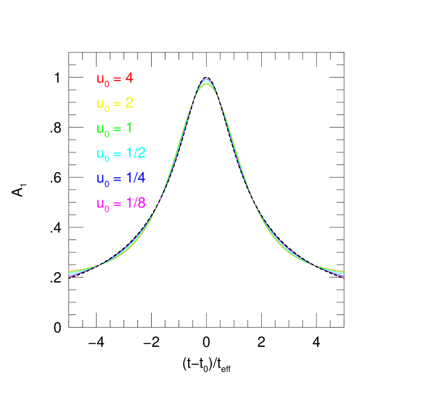
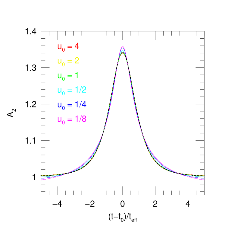
We would expect the largest $\Delta\chi^{2}$ deviation from the most coarsely sampled parameter $u_{0}$. As outlined in Section 2, $u_{0}$ is represented by just two discrete values: “high-mag” ($u_{0}\ll 1$, in effect, “$u_{0}=0$”) and $u_{0}=1$. To test the robustness of this approach, we consider light curves with $u_{0}=4,2,1,1/2,1/4,1/8$ and fit each of them to each of these two forms, i.e., by adjusting $(t_{0},t_{\rm eff})$ to get the best fit. Figure 1 shows that for $u_{0}=1/4$, the high-magnification formula $A_{1}(Q)=Q^{-1/2}$ already works extremely well, while at $u_{0}=1/8$, the input curve is almost indistinguishable from the model. On the other hand, Figure 2 shows that the $u_{0}=2$ and $u_{0}=4$ inputs are quite well fit by the $u_{0}=1$ (i.e., $A_{2}$) model. Note that $u_{0}=4$ ($A_{\rm max}\sim 1.006$) is already at, or somewhat beyond, the practical limits of microlensing detection. The most difficult case is $u_{0}=2$. This differs from both model curves by a noticeable amount, but these differences are still quite small. Since these are purely theoretical investigations, the conclusion that one of $A_{1}$ or $A_{2}$ will fit the data acceptably regardless of the true $u_{0}$ is independent of the magnitude of the event.

Next, we ask how $\Delta\chi^{2}$ is affected if the true value of $t_{0}$ differs from the model $t_{0}$ by $\epsilon t_{\rm eff}$. Note that, by construction, $\epsilon\leq\delta_{t_{0}}/2$. We can quantify the offset between the grid-based and true-model light curves by $\delta\chi^{2}/\chi^{2}$, where $\delta\chi^{2}$ is the difference between the best $\Delta\chi^{2}$ and the one that is obtained from a fit forced to $u_{0}=0$ (or $u_{0}=1$), while $\chi^{2}\equiv\sum_{i}[f_{s}(A_{i}-1)/\sigma_{i}]^{2}$. Note that (because the algorithm compares the observed lightcurve to its mean – rather than a true baseline) $\Delta\chi^{2}\sim\chi^{2}/3$. Assuming uniform cadence and below-sky errors, one finds that for high-magnification light curves $A_{1}(Q)=Q^{-1/2}$,

$${\delta\chi^{2}\over\chi^{2}}\simeq 1-{\int_{-\infty}^{\infty}dx[(1+(x-\epsilon/2)^{2})(1+(x+\epsilon/2)^{2})]^{-1/2}\over\int_{-\infty}^{\infty}dx(1+x^{2})^{-1}}\rightarrow{\epsilon^{2}\over 8}.$$ (8)

Since, as mentioned above, $\epsilon\leq\delta_{t_{0}}/2=1/6$, this ratio is negligibly small.

The $\Delta\chi^{2}$ deficit due to discretely chosen $t_{\rm eff}$ leads to a similar calculation with the result: $\delta\chi^{2}/\chi^{2}=\epsilon^{2}/32$.

The calculations of this section show that our discretization choices are, if anything, too conservative. That is, we could afford to use a coarser grid. We discuss in Section 4.9 why such conservative choices are appropriate at this stage and why they may possibly be relaxed in future years.

4 Implementation for the KMTNet 2015 Data

In addition to introducing the algorithm itself, this paper has two main goals. The first, addressed in this section, is to identify the strengths and weaknesses of the algorithm by applying it to a real data set. The second is to make available the results of the event search to the general microlensing community, which we will address further in Section 5. Both of these goals require that the algorithm be specifically applied to our data set through a series of concrete choices. One choice, for example, is whether to search for events in the data from a single observatory or whether to conduct the search by simultaneously fitting data from all three (or perhaps just two) observatories. Another choice is whether to initially vet for variable stars and artifacts by some sort of algorithm or whether to reject these totally in the operator stage “by eye”.

The actual choices made for the 2015 data were strongly conditioned by the operational environment, including both the nature of the 2015 data and the operational pressures affecting the reduction and analysis of these data. It is therefore necessary to summarize these operational constraints to understand both the empirical evaluation of the algorithm conducted below and the data products, as well as to develop ideas on how to improve application of the algorithm in the future. The last point is discussed in Section 6.

4.1 Operational Constraints

Much of the 2015 data is of very high scientific quality, and they have already been the basis of many published and submitted scientific papers (Shvartzvald et al., 2015; Bozza et al., 2016; Zhu et al., 2016; Shin et al., 2016; Han et al., 2016a, b; Zhu et al., 2017; Chung et al., 2017) However, 2015 was the commissioning year and as such it was heavily impacted by engineering tests as well as physical problems, refinements, and repairs. For example, the electronics of the KMTC camera were changed substantially on HJD${}^{\prime}\equiv{\rm HJD}-2450000=7129$ and 7192, leading to discontinuities in the photometric scale in some (but far from all) light curves at those dates. There were further experiments on the KMTC detector electronics that sometimes resulted in quite noisy data. For most of 2015, KMTS was impacted by condensation on one of the cooling lines, which triggered a short in a wallboard (before the problem was recognized) and so impacted photometry until it was replaced. And while KMTC and KMTS observations began very close to the beginning of the season (HJD${}^{\prime}\sim 7050$), KMTA began only on HJD${}^{\prime}=7180$. There were many other issues as well, including problems with the polar alignment and pointing model. Problems of this order are completely normal for the commissioning of relatively complex systems, but they also imply that algorithmic ideas that are designed for basically homogeneous data must be significantly adjusted if they are to function in this environment.

The first step was to write a pipeline to extract photometry from the images. This pipeline construction impacted the event-finder in several ways, both direct and indirect. This will be discussed in the next several subsections. However, from the present standpoint the main impact was to delay the development and testing of the event-finder. It required about 8 months to develop and test the pipeline and another 3 months, using all available computer resources, to extract light curves just for KMTC. Testing of the event-finder could proceed in parallel with light curve extraction, but full implementation could only be carried out after the light curves were extracted. Hence, event finding for 2015 did not begin in earnest until the end of the 2016 season.

The combined effect of these considerations was to drive us toward event-finding procedures that could be implemented quickly and would be robust in the face of inhomogeneous data. Work on more sophisticated versions was deferred, although this was subsequently initiated. See Section 6 for a discussion of the progress on a more advanced version.

4.2 Catalog Construction and Pipeline

The most straightforward way to extract light curves is to measure photometry at the positions of known stars. This requires a catalog of stars matched to the detector coordinate system.

The original approach that had been taken was to carry out point-spread-function (PSF) photometry using the DoPhot package (Schechter et al., 1993), which extracts a catalog directly from the images themselves. Then, those DoPhot light curves would be searched for events, and finally difference image analysis (DIA, Alard & Lupton 1998) re-reductions using the Albrow et al. (2009) pySIS package would be used for events of particular interest. This plan was well-matched to the available computer resources but suffered from what turned out to be a fatal flaw: the DoPhot-based catalogs contained a factor $\sim 5$ times fewer entries than the number of potential source stars that give rise to usable microlensing events. If not corrected, this would reduce the potential power of the experiment by roughly a factor three.

A new pipeline was written based on publicly available DIA code from Woźniak (2000). The central problem remained, however, of constructing a deep input catalog. While various packages were tried, it proved impossible to even come close to matching the depth of the existing OGLE-III (Szymański et al., 2011) catalog. The reasons for this are not completely clear. No doubt, this is partly explained by the fact that OGLE pixels are much smaller than KMTNet pixels ($0.26^{\prime\prime}$ versus $0.4^{\prime\prime}$), but it is difficult to believe that this is the full explanation. Probably the biggest factor is just greater photometric experience.

The OGLE-III catalog provides stellar positions in RA and Dec, so it was astrometrically matched to the template frame, i.e., the image coordinates, by cross-matching with the DoPhot catalog. The pipeline uses the OGLE-III catalog stars and photometric scale whenever possible. However, the OGLE-III catalog does not cover the full extent of the 2015 KMTNet fields. Some KMTNet fields cover fairly broad continuous regions that are not covered by the OGLE-III survey. In addition, the OGLE-III catalog has non-trivial topology, due to gaps of various sizes and shapes between OGLE-III fields. Approximately 10.3% of the area covered by the four prime KMTNet fields is not covered by OGLE-III (see Section 4.7). In these regions, the input catalog is derived from DoPhot templates and the photometric scale is calibrated by cross-matching with the OGLE-III catalog in nearby regions. In total, our OGLE-III + DoPhot catalog consists of 71,555,640 stars.

4.3 Automated Light Curve Search

Once the light curves for all catalog stars are extracted, they must be searched for microlensing events. Note that for 2015 data, only KMTC light curves were used to search for events (as indeed these were the only data reduced). The basic algorithm for searching for the best microlensing model was described in Section 2. Its basic features were to perform linear fits to the data on a grid of $(t_{0},t_{\rm eff},u_{0})$ and to fit only those data from the interval ($t_{0}-5\,t_{\rm eff}<t<t_{0}+5\,t_{\rm eff}$). In practice, those linear fits were performed in four phases. First, all the points were included in the fits to evaluate the best-fit parameters, $(f_{0},f_{1})$. Then, the exact procedure was repeated to determine the naive $\chi^{2}$ of each data point, using the $(f_{0},f_{1})$ from the previous step. Then the 10% worst-$\chi^{2}$ points were eliminated, and the data were refitted to redetermine $(f_{0},f_{1})$. Finally, these $(f_{0},f_{1})$ were used to determine the overall $\chi^{2}_{\rm\mu lens}$.

To determine the significance of the microlensing signal, the final sample of points (i.e., with 10% points removed) was then fitted to a flat line, i.e., a constant flux level. Nominally, this would imply a single parameter, i.e., the mean flux during the interval probed ($t_{0}-5\,t_{\rm eff}<t<t_{0}+5\,t_{\rm eff}$). In fact, however, to allow for breaks in the light curve due to firmware adjustments at KMTC, each of the three intervals described in Section 4.1 was permitted a separate mean flux level. Hence, there could be one, two, or three such parameters depending on how many of these three intervals were included in ($t_{0}-5\,t_{\rm eff}<t<t_{0}+5\,t_{\rm eff}$). This procedure yields $\chi^{2}_{\rm flat}$. Finally, the renormalized $\Delta\chi^{2}$ was derived,

$$\Delta\chi^{2}\equiv\biggl{(}{\chi^{2}_{\rm\mu lens}\over\chi^{2}_{\rm flat}}-1\biggr{)}N_{\rm data}$$ (9)

where $N_{\rm data}$ is the number of data points remaining after rejecting the worst 10%.

4.4 Automated Light Curve Grouping

Several catalog stars can yield very similar light curves, i.e., with similar $t_{0}$ and $t_{\rm eff}$. If these are produced by stars in close proximity, it may be assumed that there is only one true variable (whether microlensing or otherwise), and the other variations are simply echos of the real one. For example, there can be two catalog stars within $1^{\prime\prime}$. If one undergoes a microlensing event then when DIA is applied to the other (with $1^{\prime\prime}$ displacement of its tapered aperture), it will also generate a microlensing-like light curve. In this case, we would like to examine only the better curve, i.e., the one with higher $\Delta\chi^{2}$.

We find that in the case of bright variables (or, very occasionally, bright microlensing events) these echo light curves can extend over many tens of pixels. We therefore develop a friends-of-friends algorithm to apply to candidates found in the above search. A “friend” is defined as a light curve from another star within 10 pixels ($4^{\prime\prime}$) and with $|t_{0,1}-t_{0,2}|<0.4(t_{{\rm eff},1}+t_{{\rm eff},2})$. Then friends of friends are grouped and only the highest $\Delta\chi^{2}$ member of the group is shown to the operator. While most groups are small, it is not uncommon to have groups of several dozens, or even more than 100.

4.5 Manual Light Curve Review

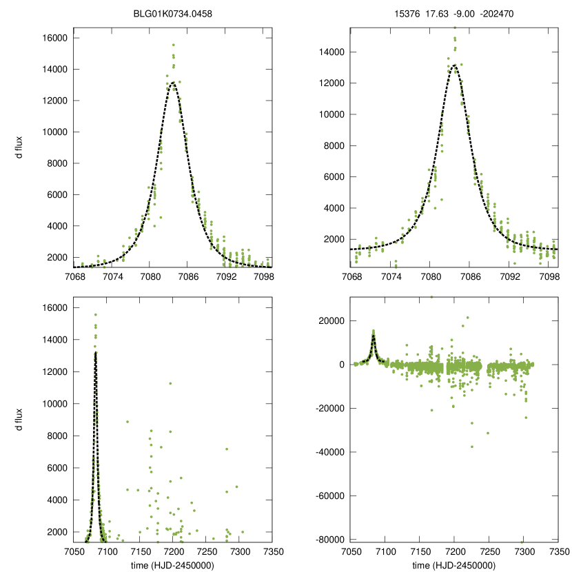
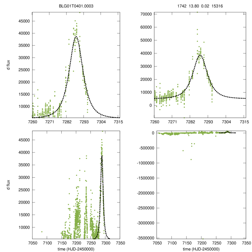
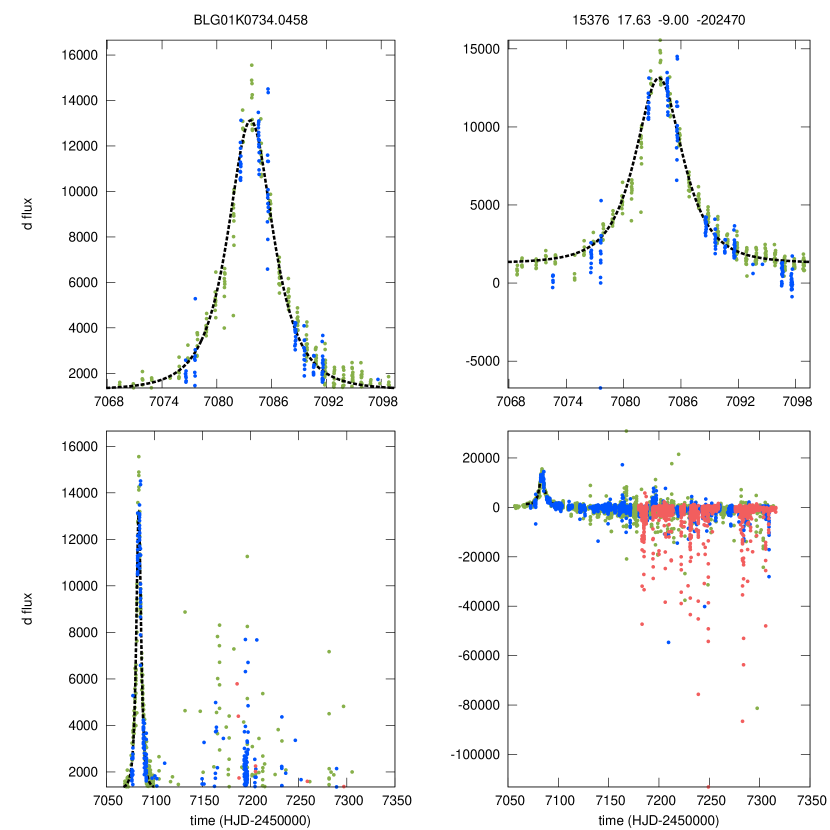
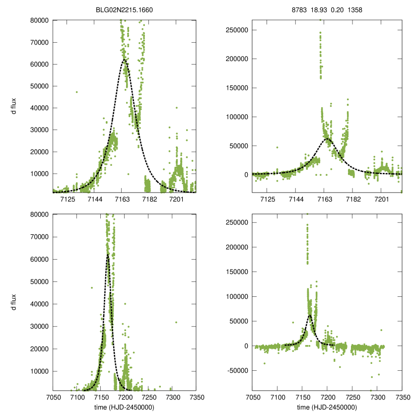
If $\Delta\chi^{2}>500$ then the candidate “event” is shown to the operator in a four-panel display, together with some auxiliary information (Figures 3–6 and Figure 11). Each panel contains all the data (not just the data surviving the 10% rejection). One reason to show all of the data is that caustic crossings in binaries are likely to be removed by the 10% rejection cut as “outliers” from the point lens fit. The bottom two panels show the whole season of data, while the top two show only the $10\,t_{\rm eff}$ that were fitted to the model. The left two panels are restricted to the flux range predicted by the model (plus small border regions at top and bottom), while the right two panels show the full range of data values within the temporal range of the diagram.

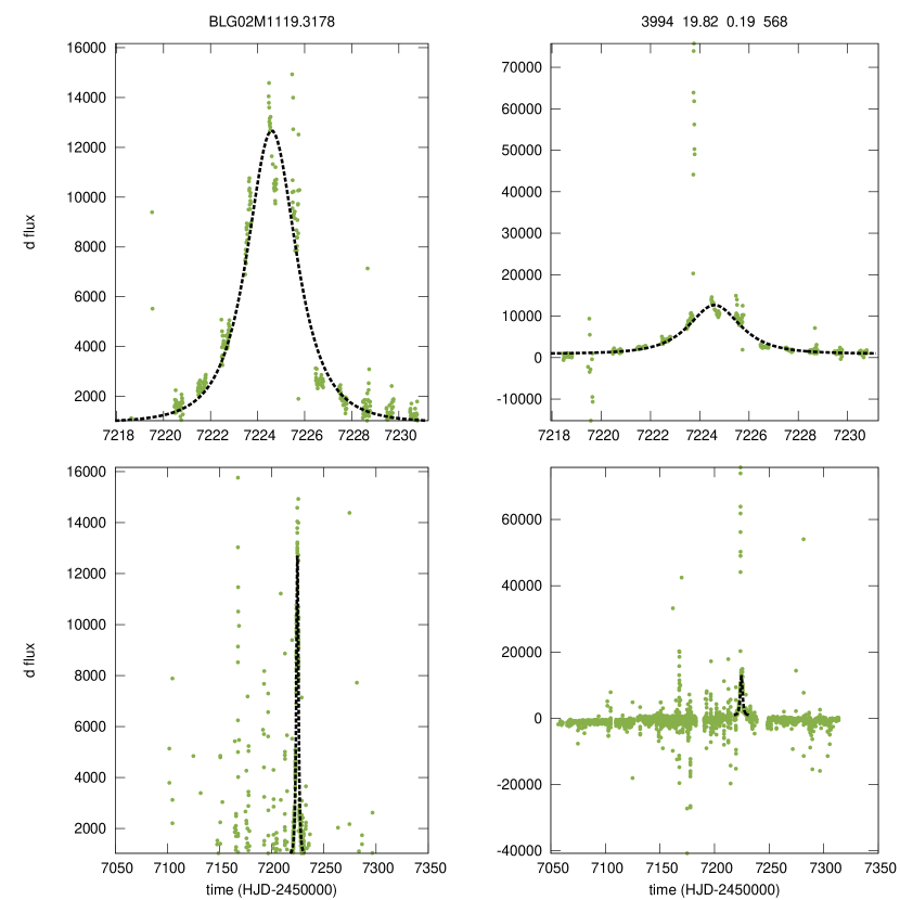
These four displays allow the operator to rapidly determine whether this is plausibly a microlensing event. For example, the upper left panel gives a very clear impression of whether the event is reasonably well fit by point lens microlensing over the $10\,t_{\rm eff}$ range that is being fit (see Figure 3). If, on the other hand, the event has pronounced binary structure (e.g., a pronounced caustic near the peak of the event), then this structure will mostly not be visible on this plot, and the light curve may appear to deviate from point-lens microlensing in an unfamiliar way. However, this caustic structure will appear clearly on the upper right panel, even if the main part of the microlensing event (easily visible on the upper left) now is so small that it is barely visible (see Figure 4).

This approach also permits rapid rejection of variables. The algorithm itself quite easily fits wide classes of variables to microlensing light curves because it “censors” data from outside the $10\,t_{\rm eff}$ fitting interval. However, this is readily apparent from the two full-season light curve panels (see Figure 5).

Above the upper-right panel are displayed four numbers $(\Delta\chi^{2},I_{\rm cat},{\rm RMS(mag)},{\rm RMS(flux)})$. Here $I_{\rm cat}$ is the magnitude of the catalog star, RMS(mag) is the amplitude of scatter of this star derived from the OGLE-III catalog, and RMS(flux) $\equiv{\rm RMS(mag)}\times 10^{0.4(28-I_{\rm cat})}$. The last number then gives the expected variability in flux units. For OGLE-III stars, $I_{\rm cat}$ is derived from the OGLE-III catalog. For non-OGLE-III stars, it is derived by calibrating the DoPhot photometry based on the overlap with OGLE-III areas. In this case, there is no information on variability, so the final two numbers are set to arbitrary negative numbers, meaning “ignore”.

The operator then classifies the candidate into one of four categories: “clear microlensing”, “possible microlensing”, “variable”, and “artifact”.

4.6 Three-Observatory Confirmation

All “clear” or “possible” microlensing events are then further evaluated using KMTS and KMTA data. As mentioned above, for 2015, only the KMTC data were reduced en masse. For candidate events, KMTS and KMTA light curves were extracted from individual $(256\times 256)$ patches cut from each image taken by these two observatories, which were then analyzed using DIA to produce light curves. These light curves are then sent through exactly the same “event-finder”, except with a threshold $\Delta\chi^{2}>0$ (instead of $\Delta\chi^{2}>500$) so that some result will be reported regardless of the quality of the fit. The operator then views all three individual displays (each with four panels) and a display with the combined data to make a final decision, again choosing from the same four categories (see Figure 6).

For genuine microlensing events, the most usual situation is that the other two observatories (or, for events before the onset of KMTA, one) have independently observed the same event and the event-finder has “found” this event and appropriately displayed it. In a few cases, the event-finder will find a “better candidate” in one of the data sets that is actually an artifact. Still it is relatively easy to check from the two full-season displays and the combined plot that the real event is present in the data. In these cases, the event can be fully confirmed as “clear” even though its KMTC-only classification is “possible microlensing”. There are some instances in which the other two observatories lack data during the candidate event’s time of significant magnification, in which case the classification must be based on KMTC data alone.

We note, however, that even when there are data from several sites, these do not constitute absolutely fool-proof security against false positives. First, eruptions by cataclysmic variables (CVs) can mimic microlensing events. Having data from several sites can help guard against these, particularly because CVs usually rise faster than microlensing events (for the same fall time) and sometimes these rises are not present in KMTC data but are present in KMTS or KMTA. However, in other cases, it can remain difficult to distinguish, either because there are few/no rising data or because the CV rises unusually slowly.

One of the biggest problems in identifying microlensing events from a single year of data is that there are no “out of year” baseline data with which to reject variables. For short events, this is not much of a problem because there are “in year” baseline data. However, there is no unambiguous way to distinguish full-season microlensing events from long-period variables. In some cases, particularly for the catalog stars derived from OGLE-III (the overwhelming majority), the variables can be vetted using “RMS(flux)”. However, this is not completely secure, since variables can remain dormant for several years or vary more in a given year than in several previous years. For the cases for which there is no obvious reason to reject the microlensing explanation, these are called “possible microlensing”.

4.7 Vetting for Artifacts by Image Inspection

A less obvious path to “false positive confirmation” comes from artifacts. Based on the commissioning issues described in Section 4.1, one can well imagine that there are a large number of artifacts in KMTC data that trigger the event finder. In the overwhelming majority of cases, these are easily recognized as such (or perhaps “misclassified” as variables) and so do not make it to the stage of vetting by KMTS and KMTA comparisons. In many of the remaining cases, these artifacts are easily removed because they are not duplicated in data from one or both of the other observatories. However, a large fraction of candidates initially classified as “possible microlensing” and a handful of those initially classified as “clear microlensing”, turn out to be examples of one of two types artifacts: “bleeding columns” and “displaced variables”. We developed simple procedures for identifying these.

For each of the events that was classified as either “clear” or “possible” microlensing, we display side-by-side the finding chart and a difference image from near the peak of the “event”. Below these are the set of light-curve displays described in Section 4.6, and below these panels are a set of four difference images: the two nearest the peak, and two other good seeing images relatively near peak.

We place cross-hairs at the catalog position of the source in all images. From the top-level difference image, one can easily see whether or not the cross hairs are at the position of the variation. If variation is not at the catalog (cross hair) position, this is not in itself a problem: many microlensing events occur on stars that are too faint to be cataloged, and are recognized by the flux variations that they induce at the position of a neighboring catalog star due to the finite width of the PSF. However, if the finding chart contains a bright star at the position corresponding to the flux variation on the difference image, then the “event” is almost certainly an artifact, i.e., an echo of variations in this bright star. Of course, a given bright star might actually undergo a microlensing event, and this event would likewise be “echoed” at the positions of neighboring cataloged stars. But in this case we would expect that the bright star would itself be cataloged and would yield a microlensing light curve with higher $\Delta\chi^{2}$. For variable sources, however, the “cleaner” light curve from the variable is much more easily excluded as a “variable” than is the “echo”, so only the echo winds up in the list of candidates.

Moreover, it is almost always the case that these echos last for most or all of the season, simply because repeating variations would have been recognized as variables, even in their echos. In the course of this vetting, we noted a handful (2–3) cases for which the source position was offset and coincident with a bright star, but the event was nevertheless short and well contained within the season. We accepted these as microlensing events and assumed that either the catalog or the event finder had failed to function properly in these cases. This means that there were probably also a few long microlensing events with similar characteristics that we misclassified as variables, but this problem cannot be addressed with only a single year of data.

Another quite common artifact that easily shows up in the difference images are fake events due to bleeding columns. In fact, the level of bleeding is far too low to be noticed directly in the images, and can only be perceived in difference images, which permit a much stronger “stretch”. Time variable bleeds can be generated by variable stars, in which case they are typically either long-timescale or repeating. However, they can also be generated by shorter-period irregular variables that only rise above the bleed threshold for a relatively short period, once in a season. In addition, they can be caused by changes in seeing and background. The former is not likely to be correlated among observatories, but the latter is, i.e., if it is due to lunar phase. In any case, as mentioned above, such bleeding columns are easily recognized by examining the four images that we routinely display.

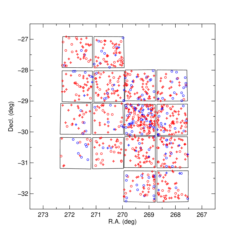
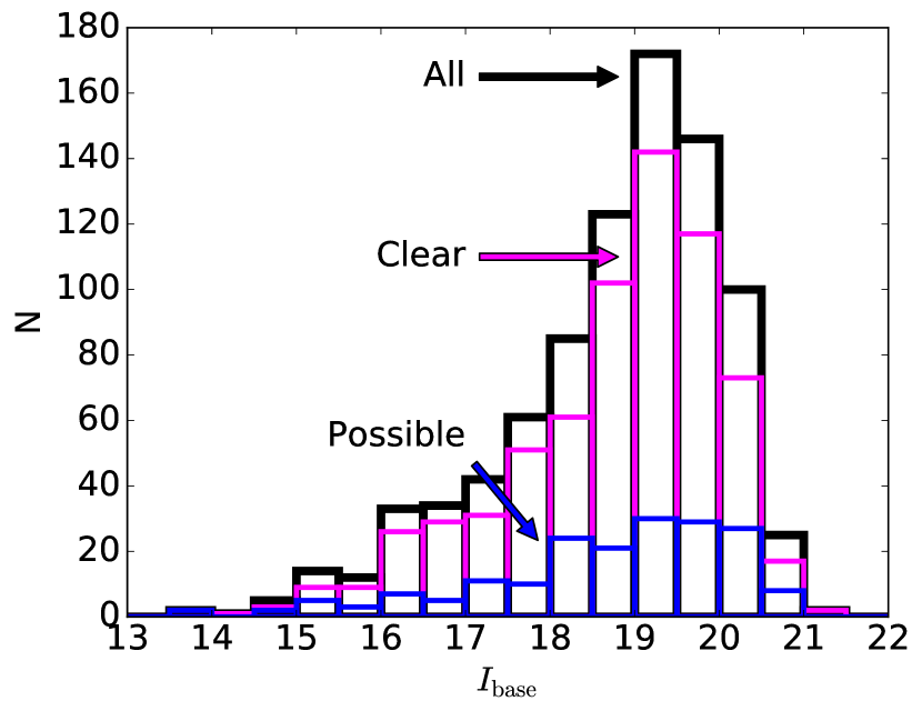
The event finder yielded 955,659 candidates, which were automatically grouped into 385,565 groups to be shown to the operator. Of these, 148,010 were classified as “variables”, and 236,698 as “artifacts”. Our final catalog of events consists of 673 “clear microlensing” and 184 “possible microlensing” events (with some duplicates). See Figure 7. Section 4.10 summarizes the properties of our final sample.

It is interesting to compare this map of detections with a map of the underlying catalog (Figure 8). Note in particular that BLG02N has a density only about 1.35 times higher than BLG04N but has an order of magnitude more “clear microlensing” events. This is broadly consistent with our expectations based on Poleski (2016), which shows that the microlensing event rate should be highest near the center of BLG02N.

4.8 Comparison to OGLE-IV EWS Detections

The best external check on the event-detection procedures described above is to compare with OGLE-IV. Since OGLE operates from a very nearby site in Chile, it has very similar field visibility and weather to KMTC, i.e., the KMTNet site used for the initial selections. In fact, the visibility is not identical because OGLE observes to greater hour angle than KMTC and also longer into austral spring. On the other hand, KMTNet observes during all lunar phases, while OGLE typically halts observations when the Moon is in the Galactic Bulge. Similarly, KMTNet observes in all atmospheric conditions, provided that these do not endanger the telescope and provided that the sky is not opaque. Further, for about a quarter of the KMTNet prime area, OGLE-IV observes with cadence $\Gamma=3\,{\rm hr}^{-1}$, which is not qualitatively different from the KMTNet cadence. And, for most of the remaining area, OGLE-IV observes with cadence $\Gamma=1\,{\rm hr}^{-1}$, which still should be sufficient to detect a substantial majority of microlensing events that are accessible to KMTNet.

For this comparison, we use the set of OGLE-IV events announced by their Early Warning System (EWS Udalski, 2003). These events are identified in real-time based on only a partial light curve rather than a full microlensing fit to a completed event. As such, this comparison sample may not be complete and it may also contain some false positives. However, it represents the most complete, publicly available, independent list of microlensing discoveries for the 2015 season.

4.8.1 OGLE-IV Events Not found by KMTNet

428 OGLE-IV events (after eliminating duplicates) in the KMTNet field were not recovered by our event finding procedure, neither as “clear” nor “possible” microlensing events. These represent potential false negatives and may indicate problems with our procedure. We first assess the fraction of the OGLE-IV alerts discovered as a function of brightness. We define $I_{\rm peak}=18-2.5*\log[f_{\rm S}(A_{\rm max}-1)]$, where $f_{\rm S}$ and $A_{\rm max}$ are determined from the OGLE EWS table. For the following ranges of $I_{\rm peak}$, we find the recovery percentages are $I_{\rm peak}(<14\,$mag$\,=63\%$, $[14$–$15]=91\%$, $[15$–$16]=76\%$, $[16$–$17]=72\%$, $[17$–$18]=72\%$, $[18$–$19]=61\%$, $[19$–$20]=43\%$, and $>20=16\%$), i.e., the events missed by our procedure tend to be biased toward the faint end.

To explore this in more detail, we examined one out of each 20 OGLE-IV events in the KMTNet fields that were not found by the procedures outlined above. This test was conducted after selection based on KMTC data, and before vetting based on KMTS and KMTA data, in order to provide the closest basis of comparison. One result of this test was that we found that three of the 22 tested events lay in image patches that had not been processed by the event-finder due to a failure in the computer architecture (and so having nothing to do with the event finder itself). These computer problems were fixed and these patches were re-run. We report only on the remaining 19 tested events.

Of these 19 “missing events”, three were clear failures, three were judged to be “marginally acceptable” false negatives, and remaining 13 were “acceptable” false negatives.

Two of the clear failures (OGLE-2015-BLG-0693 and OGLE-2015-BLG-1589) were due to operator error. The first was mislabeled as “CV”, and the second should have been called “possible microlensing” (and then further investigated using KMTS and KMTA data). The third failure (OGLE-2015-BLG-1015) lay in a thin band between two patches. Each $1\,{\rm deg}^{2}$ chip of the 2015 data was analyzed in a ($40\times 40$) grid of “overlapping” ($256\times 256$) patches, but in a few cases (given the “dead zone” boundaries imposed by the DIA software) the patches did not actually overlap. This issue is resolved for 2016+ data by going to much larger patches with much larger boundaries.

Two of the three “marginally acceptable” cases (OGLE-2015-BLG-0870 and OGLE-2015-BLG-1138) were missed because the operator judged the data to be too noisy for reliable microlensing detection. In hindsight (and knowing that there is a real event there), these might have been classified as “possible” and further investigated using KMTS and KMTA data. However, these events were quite near the threshold at which “letting in” additional events would have led to vast increase in “investigations” of pure noise and variables.

The third marginal case (OGLE-2015-BLG-1589) was not shown to the operator because $\Delta\chi^{2}=436$. If it had been shown, it probably would have been classified as “possible microlensing”. Rectification of this “problem” would require setting the threshold lower and so greatly increasing the already large number of events to be vetted.

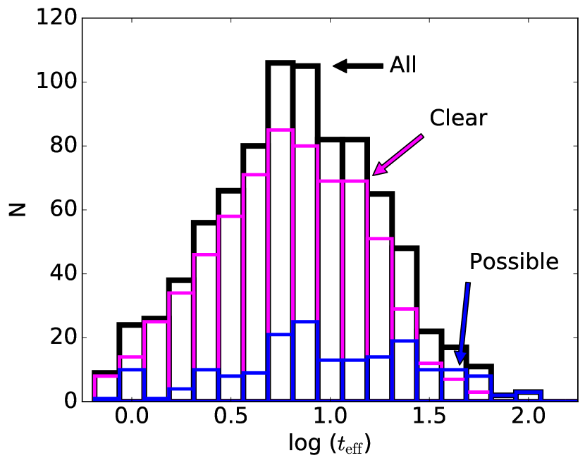
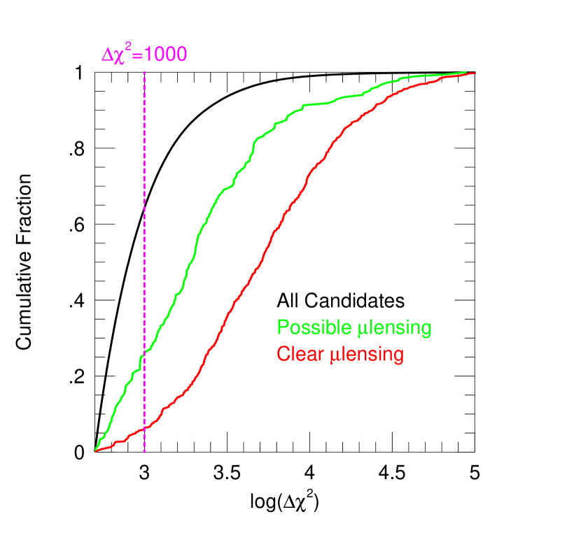
To better understand the issues involved in possibly setting a lower threshold, we show in Figure 10 cumulative distributions by $\Delta\chi^{2}$ of i) all event groups, ii) “clear microlensing” events, and iii) “possible microlensing” events. Of particular note: while 64% of all (385,565) event groups had $500<\Delta\chi^{2}<1000$, only 6.2% of “clear microlensing” events lay in this range.

The remaining 13 event non-detections were all judged to be “acceptable” false negatives. For two of these, (OGLE-2015-BLG-0059 and OGLE-2015-BLG-0960) the nearest stars in the catalog were $1.2^{\prime\prime}$ and $2.4^{\prime\prime}$, which led to very weak and no signal respectively. Neither passed the $\Delta\chi^{2}=500$ threshold, but if they had, neither would have been chosen by the operator. Both events lie in regions not covered by the OGLE-III catalog, and for which we are dependent on the much shallower DoPhot catalogs.

One event peaked midway between 2014 and 2015 seasons, and so was not recognizable based on 2015 data. Two were long events that were (correctly) judged by the operator to be consistent with being variables based on 2015 data. Two events were affected by artifacts in the 2015 data. The remaining eight had low S/N and so were not shown to the operator, but if they had been they would have been judged as too noisy for reasonable identification as microlensing events. (One of these, OGLE-2015-BLG-1835, may be a CV.)

In brief, this test shows that of order $3\times 20=60$ genuine microlensing events that could have been detected in this region were not. These failures are mostly due to “operator fatigue” from reviewing hundreds of thousands of light curves. In future years, this may be ameliorated by eliminating most variables in advance and by reduction in the number of artifacts now that commissioning is complete.

4.8.2 Events in KMTNet Not Found by OGLE-IV

For “clear microlensing” events found by KMTNet but not found by the OGLE-IV EWS, we would like to try to understand why they were not detected by OGLE-IV. For these events there are three possibilities: OGLE could not detect (or would have extreme difficulty detecting) the event due to insufficient data, OGLE excluded the event as a false positive, or the OGLE EWS missed the event. Since OGLE has a different camera, a different site, and different observing protocols, the data on a particular event might be insufficient due to the location of chip gaps or observability gaps. The OGLE survey has also been in operation for many years and so can identify (and exclude) false positives due to long-timescale, sporadic variables. We examine a representative sample of the KMTNet events not found by the OGLE EWS in greater detail to assess whether or not we expect OGLE to have detected them. If it appears that OGLE ought to have detected an event, then that event is a candidate for being a false positive, i.e. it is possible OGLE did not alert the event because they had reason to believe it was a variable star rather than microlensing. At the same time, the absence of an alert is not conclusive evidence of a false positive; the event could simply have been missed. On the other hand, if the synoptic observing information suggests that OGLE would have difficulty detecting an event, than the absence of an alert does not provide any information about whether or not an event is a false positive or real microlensing.

An unpublished study by Gould & Udalski has already determined that events detected by MOA but not by OGLE are overwhelmingly undetectable by OGLE because they are in chip gaps, outside the OGLE fields, during gaps in the data, etc. A few are variable stars that have been masked from the OGLE catalog (in this case, two of 40, P. Mróz, 2017, private communication). Thus, if an event is detected by MOA but not by OGLE, we do not investigate it further because there is likely a plausible explanation as to why it was not alerted. We then reviewed a random 10% (i.e., 18) of the 177 remaining events to assess whether or not there was sufficient data for OGLE to alert them.

We find that four of these randomly chosen 18 could not plausibly have been detected by OGLE since they were either in chip gaps or would have had very few magnified points (BLG01N.3928.2251, BLG02M.0326.3862, BLG02T.0123.2655, BLG03M.0939.0577). Four additional events were very likely missed either because they lay very near a chip edge (though formally within the chip) or because they would have had only 3 or 4 significantly magnified points. (BLG01T.2412.0089, BLG02N.2218.3192, BLG03K.3511.3254, BLG04N.3638 2631). Thus, it is not possible to draw conclusions based the absence of an OGLE alert for these $4+4=8$ events.

There were four other events that appeared to us to be probably detectable, but because they contained only 6–8 magnified points, could have plausibly been missed, perhaps due to mildly adverse conditions (BLG02T.2218.3029, BLG03N.2123.2010, BLG04K.2626.3153, BLG04T.2822.2817). Here we should keep in mind that by selecting non-OGLE events, we are biased toward such adverse circumstances.

Finally, there were six events that we thought should clearly have been detected by OGLE (BLG01K.0126.0793, BLG01M.1125.1711, BLG01N.0633.3015, BLG02N.0726.2197, BLG02N.3209.0444, BLG03T.1911.1388). Five of these six lie in OGLE fields BLG505, BLG506, or BLG512, which had OGLE cadences of $\Gamma=3\,{\rm hr}^{-1}$ in 2015. If there are false positives in our sample, these should be good candidates. In reviewing these events, we find that all look plausibly like microlensing. In all cases the $t_{\rm eff}<10\,$days and the remainder of the light curve is consistent with being flat. In all cases, all three data sets basically agree on the form of the light curve (except for the first, for which there are no KMTA data). In one case (BLG01M.1125.1711) the variation is offset from the catalog star and at the position of another resolved star, which we would generally regard as a warning sign that the resolved star is a variable and the “event” is an echo. However, as discussed in Section 4.7, we override this concern when the event is of short duration and the remainder of the season is flat. This is particularly true in the present case, for which the star that is varying is relatively faint. Hence, while any of these candidates could in principle be false positives, there is no evidence that this is the case.

Subsequent to the posting of this paper on arXiv, P. Mróz (2017, private communication) kindly provided a list of all events in OGLE high cadence fields that were recognized as variables by OGLE. This list contained one of the four we thought “likely missed” by OGLE, two of the four events that we considered “probably” should have been detected, but none of the six events that we considered should “definitely” have been detected.

4.9 Binary Detection

We expect that our approach will be efficient at detecting planetary events simply because these typically look similar to point-lens events but with relatively brief anomalies. One might be concerned that these anomalies could reduce $\Delta\chi^{2}$ and so prevent their being shown to the operator. However, recall that the 10% “worst outliers” to the point-lens-like fit are eliminated from the comparison with a flat light curve. Hence, we actually do not expect this to be an issue.

The situation is, however, quite different for binary events, many of which look nothing like point-lens events. When we devised the event-finder, we had no definite expectation of how well it would perform on binaries.

We conducted a test to evaluate this performance after the fact. We manually examined all OGLE events lying in the KMTNet fields to find those that either were, or plausibly could be binaries. We found 57 binary events announced by the OGLE EWS that lie in the KMTNet fields. Thirty-four are included in our list of microlensing events (all of them are classified as “clear”. Of the 23 that were missed, only one of these both plausibly looks like microlensing in KMTC data and failed to be shown to the operator (i.e., had $\Delta\chi^{2}<500$). This was OGLE-2015-BLG-0390, which shows a sharply rising caustic exit in KMTC data but has $\Delta\chi^{2}=265$. The reason for this low $\Delta\chi^{2}$ is that the “effective time scale” of this rise is much shorter than the 0.56 day minimum of the current search. This limit was in turn set by the large number of artifact-driven “events” that would be found in the 2015 data, which would have greatly multiplied the work of the operator.

Of the other 22 that were missed, three were due to operator error: one (OGLE-2015-BLG-0095) should have been classified as “clear” microlensing and two (OGLE-2015-BLG-1346 and OGLE-2015-BLG-2017) as “possible microlensing”. For the remaining 19, the signal in the data (whether shown to the operator or not) was not sufficient to count them as plausible microlensing events. From the perspective of understanding the algorithm, the key point is that only one known binary was missed because the algorithm itself failed to detect it.

We consider it somewhat surprising that the algorithm is working as well as it is on binaries, given that it is specifically tailored to find point-lens events. One reason for this is that the algorithm will detect pretty much any sort of bump provided that it is sufficiently pronounced and not too sharp, as illustrated by Figure 11. We suspect that the good binary sensitivity then derives from the sampling density of the 3-parameter point-lens grid described in Section 3. While this sampling density is overly conservative for detecting point lens events, it likely permits matching with sharp caustic features, allowing the detection of microlensing binaries. This conjecture can be tested in the context of the improved event finder (Section 6) by repeating the fitting procedure on known binaries with a progressively less dense grid. However, because the event finding procedure is significantly less computationally intensive than the photometry pipeline, there is no strong driver to scale back the sampling density. If the computational situation changes, this test should be performed before scaling back the sampling density.

4.10 Summary of Detected Events

In total, this procedure for identifying microlensing events from the 2015 KMTNet commissioning data resulted in 857 microlensing event candidates; 15 of which are duplicates leaving 842 event candidates. Of these, we classify 660 as “clear” microlensing events and 182 as “possible” microlensing. Based on Mróz et al. (2015) and P. Mróz (2017, private communication), we find that 40 of the “clear” microlensing events and 54 of the “possible” microlensing events were classified as variables by the OGLE collaboration. Of the remaining events, 483 “clear” events and 38 “possible” events were detected by either the OGLE EWS or the MOA alert system (or both). Thus, KMTNet has detected 137 “clear” microlensing events and 90 “possible” events not found by any other survey. Based on our investigation described in Section 4.8.2 and P. Mróz (2017, private communication), there is no evidence indicating these are false positives.

The distributions of $t_{\rm eff}$ and $I_{\rm base}$ for these events are shown in Figure 9. The reader should bear in mind that $t_{\rm eff}$ is discretely defined as described in Section 2 and therefore is not a perfect representation of the event timescale.

5 Data Policy and Data Releases

KMTNet data policy is framed by several goals, which are basically compatible but are subject to some mutual tension. First, we seek to give adequate time for the KMTNet team to publish results based on the huge amount of work required to obtain and process these data. Second, we want the KMTNet data to be exploited to the maximum extent possible, whether by KMTNet team members or others. Third, we want to promote the microlensing field by making data available to as many workers as possible. Fourth, we want to avoid overworking our team on tasks that are auxiliary to the team’s own effort to publish our results. Finally, we want to avoiding infringing on the data rights of others, whether explicitly or implicitly.

5.1 KMTNet Website

KMTNet data are available at http://kmtnet.kasi.re.kr/$\sim$ulens/event/2015/ . The main page is ordered by KMT event number in the form KMT-2015-BLG-[NNNN]. These numbers are in turn sorted by field BLG[NN] (01, 02, 03, 04), chip (K,M,N,T), patch, and star number. The “clear microlensing” events are listed first, so that all entries $\leq 0673$ are “clear” and all events $\geq 0674$ are “possible”. Each line contains the best fit event-finder parameters $(t_{0},t_{\rm eff},u_{0})$ (Equations (3) and (4)), the baseline flux, and the RA and Dec. There are also cross references to OGLE and MOA discoveries. By clicking on the event name, one can see the finding chart as well as the same 16 panels of light curve displays shown to the operator. These pages also contain links to the light curve data.

5.2 2015 Policy and Releases

Guided by the above principles, we have formulated the following policies for KMTNet data for 2015. We then outline issues that are under consideration for future years in the next section.

1) All 2015 KMTNet data remain proprietary until the acceptance for publication of this paper and all papers based on 2015 KMTNet data that are explicitly mentioned in Section 4.1.

2) Beginning immediately (i.e., before the end of the proprietary period), all light curves that are posted together with this paper (see below) can be used by anyone to prepare future papers for publication. However, during the proprietary period (see (1)), they cannot be submitted for publication, nor posted on arXiv.

3) Once the priority period ends (see (1)), papers can be submitted based on the released data. We welcome collaboration with the KMTNet team, but do not require it as a condition for publication. For the cases that we collaborate, the KMTNet team does not demand any “editorial control”, but rather simply reserves the right to withdraw from papers with which we disagree strongly enough to warrant such withdrawal.

4) If additional data processing is needed, we will either provide re-reduced light curves in exchange for co-authorship or we will provide flat-fielded “stamps” surrounding the event, provided that sufficient evidence is given to us that there is substantive progress toward publication of a paper.

5) No data will be given out for events discovered by other teams but not independently discovered by KMTNet using the algorithm presented here, unless there is explicit agreement with those teams.

The data that will be made available are

1) All the data used by the event finder for all events that were determined to be either “clear microlensing” or “possible microlensing”. Recall that these data are based on Woźniak (2000) DIA using input positions derived from a pre-constructed catalog. Hence, they are not usually of the highest quality, although sometimes they are in fact close to optimal.

2) Automated Albrow et al. (2009) pySIS reductions of all light curves. In roughly half of all cases, these reductions are better or substantially better than the reductions from (1). Unfortunately, in the other half of cases, these automated reductions either basically fail or totally fail. This means that, for a substantial fraction of events, obtaining very good or excellent light curves requires additional, by hand, reductions.

No effort will be made to rectify these or any other residual problems for the 2015 data release as a whole. As discussed in Section 4.1, the 2015 data have intrinsic problems that are not likely to propagate into future years, and our main data reduction efforts will be applied to those future-year data.

5.3 2016+ Policy and Releases

Future data policy and releases will be governed by the same principles, but will be modified based both on the experience of the 2015 release and the improved quality of 2016+ data. For 2015, we are posting light curves about 18 months after the close of the 2015 season. We hope that this time lag will be substantially improved for 2016 and further improved for 2017. Since we do not know exactly what problems we will encounter, we cannot guarantee it. However, at this point we believe that a 6-month delay is a plausible target for 2017+ data because if a paper cannot be drafted within 6 months of time the data are taken, it is likely to fall down the list of priorities as the next season of data start to become available.

For 2016, we hope to have an earlier release of the events in the Kepler K2 C9 field. (See Henderson et al. 2016 for a description of the K2 C9 project.)  For KMTNet-discovered events, these data will have no proprietary period. We will also have a public release of KMTNet data on events discovered by other teams but not discovered by KMTNet. However, for these data, we will require that prospective authors obtain permission from the other teams before using the KMTNet data for publications.

6 Future Improvements

Following the work reported here creating and implementing the 2015 event-finder algorithm, and based on this experience, numerous improvements are already being implemented for the 2016, 2017 and 2018 versions of this algorithm. They will be described more fully in the 2016 (and subsequent data release paper(s).

The first improvement is simultaneous fitting to data from all three observatories. This is straightforward in principle because all three observatories have identical input star catalogs, so one can easily cross-identify light curves of the same physical “star” (really “catalog star”, which very frequently is actually a multi-star asterism).

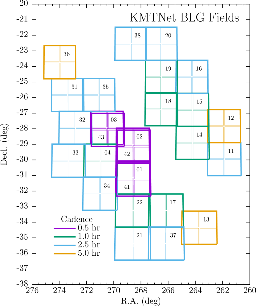
The second is simultaneous fitting of overlapping fields. This was completely unnecessary in 2015 because there were no overlapping fields. However, in 2016, each of the three “prime fields” BLG01, BLG02, BLG03, was also observed, slightly shifted, as BLG41, BLG42, BLG43, in order to cover the gaps between chips. Further, fields BLG02 and BLG03 are now somewhat overlapping in order to obtain a very high cadence on a small area $\Gamma=8\,{\rm hr}^{-1}$. Hence, there can be as many as four overlapping fields (see Figure 12). And this also means (taken together with the previous paragraph) that there can be as many as 12 light curves that might be combined. In order to reliably cross-identify stars, however, this improvement will only be implemented for OGLE-III catalog stars.

In 2015, we did not consider events with $t_{\rm eff}>99\,$days because we had no out-of-year baseline data. This will remain so in 2016 because the fields have been changed between 2015 and 2016, but also because the artifacts in the 2015 data make them unsuitable as a baseline of comparison. Such longer events can only be investigated beginning 2017.

On the other hand, it should be possible to extend the search to much shorter timescales than the 2015 limit, $t_{\rm eff}\geq 0.56\,$days. In 2015, such a search was not possible because of the large number of short timescale artifacts. It is likely that in 2016, the search will be conducted independently in the $t_{\rm eff}\geq 1\,$day and $t_{\rm eff}<1\,$day domains, to guard against long timescale events being “killed” by remaining short timescale artifacts. Finally, we note that these short timescale searches should resolve the problem found in 2015 searches of missing binary events characterized primarily by very fast rising caustics.

Experience with the 2015 data shows that it is quite difficult to reliably identify microlensing events based on the current threshold $(\Delta\chi^{2}>500)$. In 2015, we tentatively identified events from KMTC data only based on this threshold, but then relied on data from other observatories to confirm them, so the true $\Delta\chi^{2}$ was significantly higher. For 2016+, we are already using all available data for 1) OGLE-III catalog stars in all fields and 2) all stars outside of the six fields mentioned in the previous paragraph. For these, we will therefore demand $(\Delta\chi^{2}>1000)$. For the remainder (i.e., non-OGLE-III stars in BLG01, 02, 03, 41, 42, 43), we will continue to demand $(\Delta\chi^{2}>500)$.

In addition, the process of visual inspection of 2015 light curve was quite laborious. For 2016, we added automated rejection of published variables, as well as variables that were detected by KMTNet in 2015. This will remove most variables from the prime fields. For the new fields (of which there are 19), as well as the non-OGLE-III catalog stars in the prime fields, we will have to flag the variables in 2016, but then will be able to automatically censor them in future years. In 2017, we extended the rejection of cataloged KMTNet variables to all fields and added (after suitable testing) a rejection of previously found “artifacts” as well. We also introduced a new algorithm to eliminate a broad class of periodic variables, which is not a periodogram, but whose details will be described elsewhere. And we introduced a new algorithm to remove short timescale artifacts that masqueraded as short microlensing events. Again, this will be described elsewhere. Finally, for 2018, we are introducing injection of fake microlensing events into the process in order to measure the efficiency as a function of event characteristics of the entire selection process, both machine and human. See for example, Gould et al. (2006).

7 Summary

We have presented a new algorithm for finding “completed” microlensing events and described its specific application to the four, primary 2015 commissioning fields of the KMTNet microlensing survey. We find 660 “clear microlensing” events and 182 “possible microlensing” events discovered and assessed by our method. The light curves of these events will be made publicly available on our website (see Section 5.1) according to the data policy described in Section 5.2. In Section 5, we have presented our general approach to KMTNet data releases, in addition to the specific implementation of this approach for 2015 data. Feedback on the data products, data policy, etc., based on the use of these data will be helpful in preparing future releases.

Our procedure for vetting microlensing candidates still relies heavily on human inspection of the microlensing candidates. Thus, we also discuss potential modifications for future years when we expect the data to be substantially cleaner. In fact, work is currently underway to improve this algorithm for the 2016 data. Finally, we note that although the procedure for eliminating false positives will remain dependent on the specific characteristics of the data, the algorithm itself as presented in Section 2 is completely general and could be applied to diverse microlensing data sets. Indeed, Shvartzvald et al. (2017) have already applied this algorithm to find the first infrared-only microlensing events from their UKIRT survey of heavily extincted bulge regions.

Figure 1: Best-fit “high-magnification” $(u_{0}\ll 1)$ models for various values of $u_{0}=4,2,1,1/2,1/4,1/8$ from among all possible values of $(t_{0},t_{\rm eff})$. Surprisingly, even very low mag models fit reasonably well. Moreover $u_{0}\leq 1/4$ fit extremely well, and even $u_{0}=1/2$ fits quite well. Dashed black line shows the model functional form.

Figure 2: Best-fit “low-magnification” $(u_{0}=1)$ models for various values of $u_{0}=4,2,1,1/2,1/4,1/8$ from among all possible values of $(t_{0},t_{\rm eff})$. Surprisingly, even very high mag models fit reasonably well. Moreover $u_{0}\geq 1$ fit extremely well, and even $u_{0}=1/2$ fits quite well. Dashed black line shows the model functional form.

Figure 3: Example of candidate light curve (ultimately judged to be “clear microlensing”) as initially shown to the operator. Top panels show only the $10\,t_{\rm eff}\sim 30\,{\rm days}$ that were fitted to the model (dashed curve), while bottom panels show full season. Left panels show only data in the range suggested by the model curve (with small buffers at top and bottom) while right panels show the full range of data. Four numbers above the upper right panel are $\Delta\chi^{2}$, $I_{\rm base}$, variability in magnitudes, and variability in flux. Since the last two numbers are derived from the OGLE-III-catalog “rms” column, while this event comes from an area not covered by OGLE-III, these entries are negative, meaning: “ignore”.

Figure 4: Example of candidate light curve (ultimately judged to be binary “clear microlensing”) as initially shown to the operator. Panel displays are the same as in Figure 3. In this case, however, the upper right panel is crucial to realizing that the apparent “noise” near the top of the model in the upper-left panel, is actually due to a strong binary caustic entrance. Also note that since the source star is in the OGLE-III catalog, the OGLE-III “rms” (0.19 mag) is reported, and this is translated into an estimate of 568 flux units in the figures.

Figure 5: Example of candidate light curve (ultimately judged to be to be a “variable”) as initially shown to the operator. The upper left panel looks plausibly like microlensing. However, it is immediately obvious from the lower-left panel that there are several other variations during the season of similar duration, albeit of somewhat lower amplitude. The assessment of “variable” is further confirmed by the OGLE-III based “rms” of 15316 flux units. This is only slightly smaller than the rms one would measure from the “microlensing event” that is modeled in the upper-left panel.

Figure 6: Example of three-observatory light curve that the operator reviewed after the same event (shown in Figure 3) was judged to be either “clear” or “possible” microlensing. The SAAO data (blue) confirm the microlensing character previously indicated by the CTIO data (green). The SSO data start too late in the season to serve as a check in this particular case. The operator would also have been shown additional 4-panel displays for each observatory separately at this stage. Based on this inspection, the event was judged to be “clear microlensing”.

Figure 7: Four fields observed by KMTNet in 2015, BLG01, BLG02, BLG03, BLG04 each with four $1\,{\rm deg}^{2}$ chips, T, K, M, N (both counterclockwise from lower right). Red and blue indicate “clear” and “possible” microlensing. Star symbols are events found previously by OGLE and/or MOA, while circles were not previously alerted.

Figure 8: Star catalog density of four fields observed by KMTNet in 2015, BLG01, BLG02, BLG03, BLG04 each with four $1\,{\rm deg}^{2}$ chips, T, K, M, N (both counterclockwise from lower right). One per 500 catalog stars is plotted. Sharp rectangular boundaries in density are due to regions not covered by the OGLE-III catalog, where DoPhot finds only about 1/5 as many stars. Note that the catalog density is only about 1.35 times higher in BLG02N compared to BLG04N, but that there are an order of magnitude more “clear microlensing” events. See Figure 7.

Figure 9: The distribution of event detections as a function of $\log t_{\rm eff}$ (left) and $I_{\rm base}$ (right). The black solid line shows the histogram for all events; “clear microlensing” events are shown as the magenta line, and “possilbe microlensing” events are shown as the blule line.

Figure 10: Cumulative distribution functions in $\log(\Delta\chi^{2})$ for all 385,565 event groups (black), the 660 “clear microlensing” events (red) and the 182 “possible microlensing” events (green). Almost 2/3 of the event groups have $500<\Delta\chi^{2}<1000$ (left of dashed line) but these yield only 6.2% of the “clear microlensing” events.

Figure 11: Example of candidate light curve (ultimately judged to be binary “clear microlensing”). Although the event bears little resemblance to the form of point-lens microlensing (upon which the event-finder algorithm is based), it is easily selected by the algorithm $(\Delta\chi^{2}=8783)$ to be shown to the operator, who in turn easily recognized it as binary microlensing. In fact, very few recognizable binaries are rejected by the algorithm. See text.

Figure 12: 27 fields observed by KMTNet in 2016, color-coded by cadence. Note that BLG(41,42,43) are shifted by $6^{\prime}$ relative to BLG(01,02,03), which enables $\Gamma=2\,{\rm hr}^{-1}$ coverage of the chip gaps while still preserving $\Gamma=4\,{\rm hr}^{-1}$ cadence over most of this prime area. Note also that a small area is covered by four fields BLG(02,03,42,43) and so has $\Gamma=8\,{\rm hr}^{-1}$. (Courtesy of Matthew Penny).

References

- Afonso et al. (2003) Afonso, C., Albert, J. N., Alard, C., et al. 2003, A&A, 404, 145
- Alcock et al. (1993) Alcock, C., Akerlof, C.W., Alssman, R.A., et al. 1993, Nature, 365, 621
- Alcock et al. (1997) Alcock, C., Allsman, R. A., Alves, D., et al. 1997, ApJ, 479, 119
- Alard & Lupton (1998) Alard, C. & Lupton, R.H.,1998, ApJ, 503, 325
- Albrow et al. (2009) Albrow, M. D., Horne, K., Bramich, D. M., et al. 2009, MNRAS, 397, 2099
- Bond et al. (2004) Bond, I.A., Udalski, A., Jaroszyński, M. et al. 2004, ApJ, 606, L155
- Bozza et al. (2016) Bozza, V., Shvartzvald, Y., Udalski, A., et al. 2016, ApJ, 820, 79
- Chung et al. (2017) Chung, S.-J., Zhu, W., Udalski, A., et al. 2017, ApJ, in press
- Gould (1996) Gould, A. 1996, ApJ, 470, 201
- Gould & Loeb (1992) Gould, A. & Loeb, A. 1992, ApJ, 396, 104
- Gould et al. (2006) Gould, A., Dorsher, S., Gaudi, B. S., Udalski, A., 2006, Acta Astron., 56, 1
- Gould et al. (2013) Gould, A., Carey, S., & Yee, J. 2013, 2013spitz.prop.10036
- Gould et al. (2014) Gould, A., Carey, S., & Yee, J. 2014, 2014spitz.prop.11006
- Gould et al. (2015a) Gould, A., Yee, J., & Carey, S., 2015a, 2015spitz.prop.12013
- Gould et al. (2015b) Gould, A., Yee, J., & Carey, S., 2015b, 2015spitz.prop.12015
- Gould et al. (2016) Gould, A., Yee, J., & Carey, S., 2016, 2016spitz.prop.13005
- Hamadache et al. (2006) Hamadache, C., Le Guillou, L., Tisserand, et al. 2006, A&A, 454, 185
- Han et al. (2016a) Han, C., Udalski, A., Lee, C.-U., et al. 2016a, ApJ, 827, 11
- Han et al. (2016b) Han, C., Udalski, A., Gould, A., et al. 2016b, AJ, 152, 95
- Henderson et al. (2016) Henderson, C.B., Poleski, R., Penny, M. et al. 2016 PASP128, 124401
- Kim et al. (2016) Kim, S.-L., Lee, C.-U., Park, B.-G., et al. 2016, JKAS, 49, 37
- Mróz et al. (2015) Mróz, P., Udalski, A., Poleski, R., et al. 2015, Acta Astron., 65, 313
- Poleski et al. (2014) Poleski, R., Udalski, A., Dong, S. et al. 2014, ApJ, 782, 47
- Poleski (2016) Poleski, R., 2016, MNRAS, 455, 3656
- Schechter et al. (1993) Schechter, P.L., Mateo, M., & Saha, A. 1993, PASP, 105, 1342
- Shin et al. (2016) Shin, I.-G., Ryu, Y.H, Udalski, A. et al. 2016, JKAS, 49, 73
- Shvartzvald & Maoz (2012) Shvartzvald, Y., Maoz, D. 2012, MNRAS, 419, 3631
- Shvartzvald et al. (2014) Shvartzvald, Y., Maoz, D., Kaspi, S., et al. 2014, MNRAS, 439, 604
- Shvartzvald et al. (2015) Shvartzvald, Y., Udalski, A., Gould, A. et al. 2015, ApJ, 814, 111
- Shvartzvald et al. (2017) Shvartzvald, Y., Bryden, G., Gould, A. et al. 2017, AJ, 153, 61
- Szymański et al. (2011) Szymański, M.K., Udalski, A., Soszyński, I., et al. 2011, Acta Astron., 61, 83
- Udalski (2003) Udalski, A. 2003, Acta Astron., 53, 291
- Udalski et al. (1994) Udalski, A., Szymanski, M., Kaluzny, J., Kubiak, M., Mateo, M., Krzeminski, W., & Paczyński, B. 1994, Acta Astron., 44, 317
- Udalski et al. (2015) Udalski, A., Yee, J.C., Gould, A., et al. 2015, ApJ, 799, 237
- Woźniak (2000) Woźniak, P. R. 2000, Acta Astron., 50, 421
- Wyrzykowski, Ł., et al. (2009) Wyrzykowski, Ł., Kozłowski, S., Skowron, J., et al. 2009, MNRAS, 397, 1228
- Wyrzykowski et al. (2010) Wyrzykowski, Ł., Kozłowski, S., Skowron, J., et al. 2010, MNRAS, 407, 189
- Wyrzykowski et al. (2011a) Wyrzykowski, Ł., Kozłowski, S., Skowron, J., et al. 2011, MNRAS, 413, 493
- Wyrzykowski et al. (2011b) Wyrzykowski, L., Skowron, J., Kozłowski, et al. 2011, MNRAS, 416, 2949
- Wyrzykowski et al. (2015) Wyrzykowski, Ł., Rynkiewicz, A.E., Skowron, J., et al. 2015, ApJS, 216, 12
- Yee et al. (2015) Yee, J.C., Gould, A., Beichman, C., 2015, ApJ, 810, 155
- Zhu et al. (2016) Zhu, Wei; Calchi Novati, S.; Gould, A. et al., 2016, ApJ, 825, 60
- Zhu et al. (2017) Zhu, W., Udalski, A., Calchi Novati, S, et al. 2017, AJ, in press, arXiv:1701.05191