OGLE-2017-BLG-1434Lb: Eighth $q<1\times 10^{-4}$ Mass-Ratio Microlens Planet Confirms Turnover in Planet Mass-Ratio Function

Abstract

We report the discovery of a cold Super-Earth planet ($m_{p}=4.4\pm 0.5\,M_{\oplus}$) orbiting a low-mass ($M=0.23\pm 0.03\,M_{\odot}$) M dwarf at projected separation $a_{\perp}=1.18\,\pm 0.10$ AU, i.e., about $1.9$ times the snow line. The system is quite nearby for a microlensing planet, $D_{L}=0.86\pm 0.09\,{\rm kpc}$. Indeed, it was the large lens-source relative parallax $\pi_{\rm rel}=1.0\,{\rm mas}$ (combined with the low mass $M$) that gave rise to the large, and thus well-measured, “microlens parallax” $\pi_{\rm E}\propto(\pi_{\rm rel}/M)^{1/2}$ that enabled these precise measurements. OGLE-2017-BLG-1434Lb is the eighth microlensing planet with planet-host mass ratio $q<1\times 10^{-4}$. We apply a new planet-detection sensitivity method, which is a variant of “$V/V_{\rm max}$”, to seven of these eight planets to derive the mass-ratio function in this regime. We find $dN/d\ln q\propto q^{p}$, with $p=1.05^{+0.78}_{-0.68}$, which confirms the “turnover” in the mass function found by Suzuki et al. (2016) relative to the power law of opposite sign $n=-0.93\pm 0.13$ at higher mass ratios $q\gtrsim 2\times 10^{-4}$. We combine our result with that of Suzuki et al. (2016) to obtain $p=0.73^{+0.42}_{-0.34}$.

1 Introduction

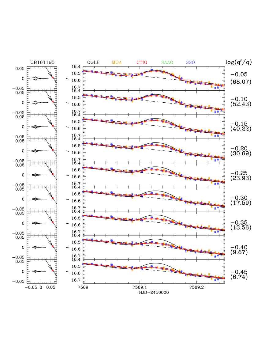
Figure 7: Nine simulations of OGLE-2016-BLG-1195, similar to Figure 4, except that in this case the data points are based on the re-reduced data in order to focus on whether the event (once recognized as interesting) would be publishable.

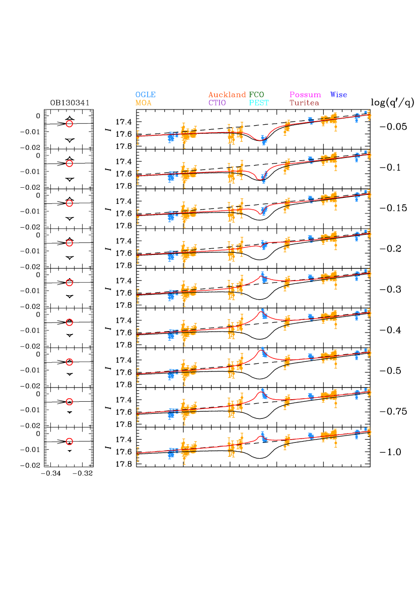
Figure 8: Nine simulations of OGLE-2013-BLG-0341, similar to Figure 4. Similar to those simulations, it is based on “online” OGLE and MOA data in order to focus on the problem of real-time recognition of the planetary anomaly.

Microlensing searches are finding planets with planet/host mass ratio $q$ that are nearly uniformly distributed in $\log q$ over $-4.3\lesssim\log q\lesssim-2$ (Figures 7 and 8 of Mróz et al. 2017). Since planet detectability grows with $q$, this immediately implies a steeply rising mass function toward lower mass ratios. In the first study to measure this relation, Sumi et al. (2010) found $dN/d\log q\propto q^{n}$ with $n=-0.7\pm 0.2$. Naively, the almost perfectly flat distribution cataloged by Mróz et al. (2017) over a 2.3 dex range in $q$ would indeed appear to argue for a single power law. However, Suzuki et al. (2016) subsequently argued for a break in the power law at about $\log q\sim-3.75$, with $n=-0.93\pm 0.13$ above the break. Below the break they found a sign reversal in the power law, $dN/d\log q\propto q^{p}$ with $p=0.6^{+0.5}_{-0.4}$, implying a true “turnover” at the break. The main argument for this break is that existing planet surveys had significant sensitivity to planets below the break, but found very few. In particular, the Microlensing Observations in Astrophysics (MOA) survey, which was the primary data set that they analyzed, had only two planets with $\log q<-4$. Note, however, that another recent study by Shvartzvald et al. (2016), based on the overlap of the OGLE, MOA and Wise surveys, fit to a single power law and found $n=-0.50\pm 0.17$.

A confirmation and refined measurement (or, alternatively, refutation) of the Suzuki et al. (2016) break and turnover would be of great interest to constrain theories of planetary formation. Moreover, it would also be of immediate practical interest in devising strategies for WFIRST microlensing observations (Spergel et al., 2013). Since WFIRST will be far more sensitive to planets below the Suzuki et al. (2016) break than ground-based surveys, its planet discovery rate is much more sensitive to such a break.

Here, we report the discovery of the low mass ratio $q=5.8\times 10^{-5}$ planet OGLE-2017-BLG-1434Lb. This is the eighth microlensing planet with a mass ratio that is securely in the range $\log q<-4$, meaning that the sample that lies clearly below the Suzuki et al. (2016) break is now large enough for robust statistical investigation. On the other hand, in contrast to the Suzuki et al. (2016) sample, these eight planets are drawn from quite heterogeneous detection processes. Therefore proper statistical analysis requires great care.

There are two other notable features of the discovery of OGLE-2017-BLG-1434Lb. First, we are able to make an accurate mass measurement, thanks to a clear detection of the microlens parallax parameter,

$${\mbox{\boldmath$\pi$}}_{\rm E}\equiv\pi_{\rm E}{{\mbox{\boldmath$\mu$}}_{\rm rel}\over\mu_{\rm rel}},\qquad\pi_{\rm E}\equiv{\pi_{\rm rel}\over\theta_{\rm E}};$$ (1)

where $\pi_{\rm rel}\equiv{\rm AU}(D_{L}^{-1}-D_{S}^{-1})$ and ${\mbox{\boldmath$\mu$}}_{\rm rel}$ are the lens-source relative parallax and proper motion, respectively,

$$\theta_{\rm E}\equiv\sqrt{\kappa M\pi_{\rm rel}};\qquad\kappa\equiv{4G\over c^{2}{\rm AU}}\simeq 8.14{{\rm mas}\over M_{\odot}},$$ (2)

and $M$ is the lens mass. Note that when $\pi_{\rm E}$ and $\theta_{\rm E}$ are both measured, $M=\theta_{\rm E}/\kappa\pi_{\rm E}$ can likewise be determined (Gould, 1992, 2000, 2004; Gould & Horne, 2013).

Of the eight planets with $\log q<-4$, five have good-to-excellent mass measurements, which is a remarkably high fraction. Two of these (including OGLE-2017-BLG-1434) have excellent ground-based parallax measurements, one has a good ground-based parallax measurement, one has an excellent space-based parallax measurement using Spitzer, and for the last, the host was directly imaged 8.2 years after the event. This high rate of mass measurements permits at least a qualitative statement about the distribution of host masses of low mass-ratio planets.

Second, although OGLE-2017-BLG-1434 is within a factor 1.3 of the lowest mass-ratio microlensing planet, we show that it would have been both detected and well-characterized even if it were a factor 30 smaller in $q$, i.e., $\log q=-5.71$, or approximately 12 Moon masses. This demonstrates that microlensing studies, at least in their current configuration, can probe to substantially smaller masses than have yet been reported as discoveries, and hence further motivates an investigation of whether there is really a break in the mass-ratio function near $\log q\sim-4$.

2 Observations

OGLE-2017-BLG-1434 is at (RA,Dec)_J2000 = (17:53:07.29,$-30$:14:44.6), corresponding to $(l,b)=(-0.28,-2.07)$. It was discovered and announced as a probable microlensing event by the OGLE Early Warning System (Udalski et al., 1994; Udalski, 2003) at UT 19:33 25 Jul 2017. The event lies in OGLE field BLG501, for which OGLE observations were at a cadence of $\Gamma=1\,{\rm hr^{-1}}$ during the 2017 season using their 1.3m telescope at Las Campanas, Chile.

The Korea Microlensing Telescope Network (KMTNet, Kim et al. 2016) observed this field from its three 1.6m telescopes at CTIO (Chile, KMTC), SAAO (South Africa, KMTS) and SSO (Australia, KMTA), in its two slightly offset fields BLG01 and BLG41, with combined cadence of $\Gamma=4\,{\rm hr^{-1}}$ .

The great majority of these survey observations were carried out in $I$ band with occasional $V$ band observations made solely to determine source colors. All reductions for the light curve analysis were conducted using variants of difference image analysis (DIA, Alard & Lupton 1998), specifically Woźniak (2000) and Albrow et al. (2009).

The MiNDSTEp collaboration observed OGLE-2017-BLG-1434 from the 1.54m Danish Telescope at La Silla, Chile, using an EMCCD camera operated at 10 Hz and with a broad passband approximating the $I$-band filter, with mean response at 770 nm (Skottfelt et al., 2015; Evans et al., 2016). The data were reduced using an updated version of the DanDIA pipeline (Bramich, 2008). These observations were initiated with 10 exposures on the night of ${\rm HJD}^{\prime}=7981$ and continually increased to 75 exposures on ${\rm HJD}^{\prime}=7984$, i.e., the night closest to the predicted peak, falling to 50 exposures the following night. Based on these last observations, MiNDSTEp issued an alert, triggered by SIGNALMEN (Dominik et al., 2007), of a possible anomaly, which it confirmed the next day based on OGLE online data. MiNDSTEp then continued regular observations of the event until the night of ${\rm HJD}^{\prime}=7998$.

3 Analysis

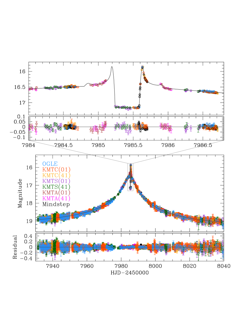
Figure 1: Light curve and best-fit model of OGLE-2017-BLG-1434. As discussed in Section 3, many of the key parameters can be “read off” the light curve, including that this is a very low mass-ratio planet: $q<10^{-4}$. Data are color-coded by observatory.

With the exception of some deviations near the peak that last slightly more than one day, the overall shape of the OGLE-2017-BLG-1434 light curve (Figure 1) is that of an ordinary point-lens (Paczyński, 1986) event. Excluding the deviation, the change in magnitude from baseline to peak ($\sim 2.5$ mag) implies a magnification $A\gtrsim 10$ (higher if there is significant blending). The two most obvious components of the deviation are a flat trough that lies about 0.7 mag below the level of the point-lens curve and lasts 0.4 days (traced in KMTS, OGLE, KMTC, and MiNDSTEp data), followed by a very rapid caustic entrance (traced in KMTC, OGLE, and MiNDSTEp data). Once these features are noted, it becomes clear that the underlying light curve is essentially symmetric and that the onset of a caustic exit is traced by KMTA data just before the trough.

This trough is an unambiguous signature of a “minor image perturbation”. The point-lens light curve (due to the host in the absence of a companion) is generated by two images of the source. The major image forms at a minimum in the time-delay surface (in accord with Fermat’s principle), while the minor image forms at a saddle point. The latter is highly unstable, so that if a small planet lies at or near the position of this image, the image will be virtually annihilated. The flux ratio of the two images is $\eta=(A-1)/(A+1)$ where $A$ is the total magnification. Hence, for a high-magnification event such as this one, $\eta\rightarrow 1$, which means that annihilating the minor image should decrease the total flux by half, i.e. $\sim 0.75$ mag. That is, the light curve’s behavior exactly corresponds to this expectation.

Such troughs are always aligned with the planet-star axis and are flanked by two caustics. However, the troughs generally extend substantially beyond the caustics. Hence, if the source trajectory crosses the trough at a point where there are no caustics, its entrance and exit to the trough will be smooth. However, if it crosses the caustics, the trough entrance and exit will correspond to a sharp (discontinuous slope) caustic exit and entrance, respectively. The latter is clearly the geometry of OGLE-2017-BLG-1434.

Of course, after exiting the trough (so, entering the caustic), the source must again exit the caustic. Because the caustic edge facing the trough is much stronger than its “outer walls”, the effect on the light curve is much less pronounced. Nevertheless, this outer-edge crossing was captured in the first three KMTA points after the trough.

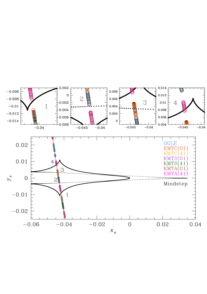
Figure 2: Caustic diagram of OGLE-2017-BLG-1434. The source passes over the “planetary wing” of a resonant caustic, resulting from the planet perturbing the minor image. The points are color coded by observatory, and their size represents the scaled source $\rho=4.5\times 10^{-4}$ of the best fit model.

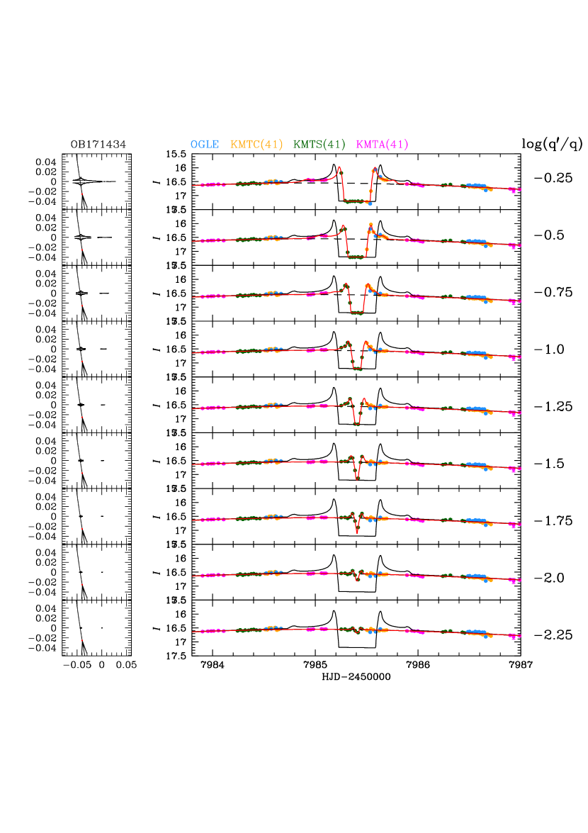
Figure 4: Nine simulations of OGLE-2017-BLG-1434 with exactly the same parameters as the best-fit model (black curve) except that the mass ratio $q$ is lower by $\Delta\log q$ as indicated in the right axis labels. In each case, the simulated data points (various colors) deviate from the model (orange curve) by exactly the same amount as the actual data points deviate from the best-fit model. The left panels show the corresponding caustic geometries. These characteristics will be same for all eight events in the figures that follow. In this figure, the data points are based on the “online” OGLE data and “quick look” KMTNet data in order to focus on the problem of determining whether the event would be recognized as sufficiently interesting to trigger re-reductions.

If the trough occurs at relatively low magnification, then each of the two caustic “walls” that flank the caustic will be part of triangular caustic structures. However, at progressively higher magnification (corresponding to planets that are progressively closer to the Einstein ring), these triangular caustics grow in size and progressively move toward the quadrilateral central caustic close to the host. The triangular caustics eventually merge with the central caustic to form a single, six-sided caustic (Figure 4 of Gaudi 2012). This turns out to be the geometry of OGLE-2017-BLG-1434. See Figure 2.

Continuing this logic, one can approximately read off the parameters of a standard seven-parameter model from the light curve, using known analytic formula (Han, 2006) for the caustics. Three of these parameters $(t_{0},u_{0},t_{\rm E})$ correspond to the time of maximum, impact parameter, and Einstein crossing time of the underlying point-lens (Paczyński, 1986) model. Three others $(s,q,\alpha)$ describe the binary companion, namely its separation (in units of $\theta_{\rm E}$), its mass ratio, and the angle of the binary axis relative to the source trajectory. Finally, if (as in the present case) the source passes over or near the caustics, one must specify $\rho=\theta_{*}/\theta_{\rm E}$, i.e., the ratio of the source radius to the Einstein radius.

A point-lens fit to the light curve with the anomaly removed yields $(t_{0},u_{0},t_{\rm E})=(7984.94,0.027,95\,{\rm day})$, which implies an effective timescale $t_{\rm eff}\equiv u_{0}t_{\rm E}=2.57\,$ days. The anomaly is centered $\delta t=0.5\,$days after peak, implying that $\alpha={\rm atan}(-t_{\rm eff}/\delta t)=\pm 259^{\circ}$ and that $s$ should satisfy, $s^{-1}-s=u_{0}\sqrt{1+(\delta t/t_{\rm eff})^{2}}$, which implies $s\simeq 1-u_{0}/2=0.986$. From the light curve, the duration of the trough is $\Delta t\simeq 0.4\,$days. (It could in principle be slightly larger because the caustic exit is not actually observed. However, the rise toward the caustic is observed from KMTA, so this estimate cannot be far off.) This quantity can be related to the Han (2006) parameter $\eta_{c-}=2q^{1/2}(s^{-2}-1)^{1/2}$ by $\Delta t=2t_{\rm E}\eta_{c-}|\sec\alpha|$, which for the present case implies $q\simeq u_{0}(\Delta t/t_{\rm eff})^{2}/16=4.1\times 10^{-5}$. Finally, the rise time of the caustic exit in OGLE/KMTC/MiNDSTEp data is $t_{\rm rise}=66\,$min. From Gould & Andronov (1999), $t_{\rm rise}=1.7\,t_{*}\sec\alpha$, where $t_{*}=\rho t_{\rm E}$. Hence, $t_{*}=39\,$min and $\rho\simeq(t_{*}/t_{\rm E})=3.5\times 10^{-4}$.

However, following from these results, it is obvious that additional higher order effects should be measurable. First note that $\rho$ is unusually small, so that the Einstein radius $\theta_{\rm E}=\theta_{*}/\rho\simeq 3000\,\theta_{*}$. We will estimate the source size $\theta_{*}$ in detail in Section 4.1. However, just from the source flux derived from the Paczyński (1986) fit, it is an upper main sequence star, i.e., $\theta_{*}\sim 0.5\,\mu{\rm as}$.

Such a large Einstein radius $(\theta_{\rm E}\sim 1.5\,{\rm mas})$ immediately implies that the host must be either a dark remnant (black hole or neutron star) or it must be quite nearby. That is, from the definition of $\theta_{\rm E}$ (Equation (2)),

$$\pi_{\rm rel}={\theta_{\rm E}^{2}\over\kappa M}\rightarrow 0.3\,{\rm mas}\bigg{(}{M\over M_{\odot}}\biggr{)}^{-1}.$$ (3)

Indeed, since a solar-mass star at $D_{L}\sim 2.5\,{\rm kpc}$ would easily be visible, the actual lens must have even lower mass (hence higher $\pi_{\rm rel}$). Therefore, again unless the host is a dark remnant, the microlens parallax must be fairly large.

$$\pi_{\rm E}={\pi_{\rm rel}\over\theta_{\rm E}}>0.2.$$ (4)

Given that the event is quite long, such a parallax should be measurable.

Thus, without any detailed modeling, one can infer that there should be a strong microlens parallax signal and that the implications of not finding such a signal would be striking.

When introducing the two parallax parameters ${\mbox{\boldmath$\pi$}}_{\rm E}=(\pi_{{\rm E},N},\pi_{{\rm E},E})$, one must also, at least initially, introduce linearized orbital motion parameters $(ds/dt,d\alpha/dt)$ as well. These encode the instantaneous rate of change in the separation and orientation of the binary at $t_{0}$. There are two reasons that these must be included. First, the orbital motion parameters $(ds/dt,d\alpha/dt)$ can be correlated with ${\mbox{\boldmath$\pi$}}_{\rm E}$, so that by ignoring them one can induce artificial effects in the parallax (Skowron et al., 2011; Batista et al., 2011; Han et al., 2016). Second, binary systems are known a priori to orbit their center of mass. Hence, there is no viable reason for excluding these parameters except if they are better constrained by the fact that physical systems ought to be bound than they are by the data. However, while (as described above) there are very strong reasons to believe that the parallax parameters can be measured, there is no corresponding confidence with respect to $(ds/dt,d\alpha/dt)$. Therefore, these parameters must be handled carefully. See, e.g., Ryu et al. (2017).

Notwithstanding the above analytic arguments, we conduct a grid search over $(s,q,\alpha)$, seeded by the above values of $(t_{0},u_{0},t_{\rm E},\rho)$, with all parameters except $(s,q)$ allowed to vary and apply $\chi^{2}$ minimization using a Markov Chain Monte Carlo (MCMC). To evaluate the magnifications at individual data points, we use inverse ray shooting in and near the caustics (Kayser et al., 1986; Schneider & Weiss, 1988; Wambsganss, 1997) and multipole approximations (Pejcha & Heyrovský, 2009; Gould, 2008) elsewhere. We employ a linear limb-darkening coefficient $\Gamma_{I}=0.429$ based on the source type derived in Section 4.1.

We find only one solution. This is close to the one derived above analytically in terms of $(s,\alpha)$ and the so-called invariant quantities (Yee et al., 2012; Ryu et al., 2017): $(s,\alpha,t_{\rm eff},t_{*},qt_{\rm E})=[0.981,259^{\circ},(2.59,0.0284,0.00364)\,{\rm day}]$ compared to $[0.986,259^{\circ},(2.57,0.0271,0.00389)\,{\rm day}]$ “predicted”. The major difference is only in $t_{\rm E}$, which can be significantly impacted by unmodeled parallax for long timescale events.

We then introduce the higher-order parameters ${\mbox{\boldmath$\pi$}}_{\rm E}=(\pi_{{\rm E},N},\pi_{{\rm E},E})$ and ${\mbox{\boldmath$\gamma$}}=((ds/dt)/s,d\alpha/dt)$. We find that in a completely free fit, three of these are well constrained, but the fourth $(\gamma_{\perp}=d\alpha/dt)$ is not. In particular, we find that for most of the solution space, the (absolute value of the) ratio of projected kinetic to potential energy,

$$\beta\equiv\biggl{(}{\rm KE\over PE}\biggr{)}_{\perp}={\kappa\,M_{\odot}\,{\rm yr}^{2}\over 8\pi^{2}}\,{\pi_{\rm E}\over\theta_{\rm E}}\,{s^{3}\gamma^{2}\over(\pi_{\rm E}+\pi_{s}/\theta_{\rm E})^{3}},$$ (5)

violates the boundedness condition, $\beta<1$. Here, we adopt $\pi_{s}=0.117\,{\rm mas}$ for the source parallax. We address this by making two different calculations. First, we arbitrarily set ${\mbox{\boldmath$\gamma$}}=0$. Of course, as mentioned above, this is unphysical, but it is simple and is useful as a benchmark for the second calculation, in which we allow $\gamma$ to vary but restrict $\beta<0.7$, i.e., a limit that would be satisfied by the overwhelming majority of real, bound systems.

The results are shown in Table 1. The first point is that the parallax+orbital models in which $\beta$ is restricted to a reasonable physical range $\beta<0.7$ yield statistically indistinguishable results from the parallax-only models in which $\beta=\gamma=0$. That is, our inability to fully measure $\gamma$ does not significantly influence the measurement of any other parameter.

Second, while there are two degenerate $(\pm u_{0})$ models with similar $\chi^{2}$, their parameters (apart from the sign of $u_{0}$) are the same within $1\,\sigma$. Hence, this degeneracy does not materially impact the inferred physical parameters of the system.

4 Physical Parameters

4.1 Measurement of $\theta_{\rm E}$ and $\mu$

We derive the source brightness from the model presented in Section 3 and derive the color from regression. We then find the offset from the clump on an instrumental color-magnitude diagram: $[(V-I),I]_{s}-[(V-I),I]_{\rm clump}=(-0.328,+3.990)\pm(0.023,0.038)$. We adopt $[(V-I),I]_{\rm clump}=(1.06,14.46)$ from Bensby et al. (2013) and Nataf et al. (2013), respectively, and so derive $[(V-I),I]_{s}=(0.732,18.45)\pm(0.025,0.063)$. We convert from $V/I$ to $V/K$ using the $VIK$ color-color relations of Bessell & Brett (1988) and finally derive

$$\theta_{*}=0.657\pm 0.041\,\mu{\rm as}$$ (6)

using the color/surface-brightness relations of Kervella et al. (2004). Incorporating parameters from Table 1, we thereby derive.

$$\theta_{\rm E}={\theta_{*}\over\rho}=1.40\pm 0.09\,{\rm mas};\qquad\mu={\theta_{*}\over t_{\rm E}}=8.1\pm 0.5\,{\rm mas}\,{\rm yr}^{-1}.$$ (7)

4.2 Masses, Distance, and Projected Separation

Combining the results of Section 4.1 and Table 1, we find

$$M={\theta_{\rm E}\over\kappa\pi_{\rm E}}=0.234\pm 0.026\,M_{\odot};\qquad m_{p}={q\over 1+q}M=4.4\pm 0.5\,M_{\oplus}$$ (8)

and

$$D_{L}={{\rm AU}\over\theta_{\rm E}\pi_{\rm E}+\pi_{s}}=0.86\pm 0.09\,{\rm kpc}\qquad a_{\perp}=s\theta_{\rm E}D_{L}=1.18\pm 0.10\,{\rm AU},$$ (9)

where we have adopted a source parallax $\pi_{s}=0.117\pm 0.010\,{\rm mas}$ and where $a_{\perp}$ is the projected separation. That is, the planet is a super-Earth orbiting a middle-late M dwarf. If we adopt a “snow line” scaled to host mass (e.g., Kennedy & Kenyon 2008), and anchored in the observed Solar-system value, $a_{\rm snow}=2.7\,{\rm AU}\,(M/M_{\odot})$, then this planet lies projected at $a_{\perp}=1.9\,a_{\rm snow}$.

5 Microlensing Earths and Super-Earths with Well-Measured Masses

OGLE-2017-BLG-1434Lb joins a small list of Earths and Super-Earths with well-measured masses discovered by microlensing. To be an “Earth or Super-Earth”, we require a best-estimated planet mass $m_{p}<7\,M_{\oplus}$. To be “well-measured” we set two requirements. First we require that the quoted $1\,\sigma$ error on the planet mass measurement span a factor $<2$, i.e., $\sigma(\log(m_{p}))<0.15$. Second, we require that the host mass was determined either by measuring both $\pi_{\rm E}$ and $\theta_{\rm E}$ (as was done here) or by directly imaging the host.

We review the literature (effectively updating the summary by Mróz et al. 2017) and find only three such planets: OGLE-2016-BLG-1195Lb (Bond et al., 2017; Shvartzvald et al., 2017), OGLE-2013-BLG-0341LBb (Gould et al., 2014), and OGLE-2017-BLG-1434Lb (this work). In all cases, the mass determination is via measurements of $\theta_{\rm E}$ and $\pi_{\rm E}$. We note that there is another planet, MOA-2007-BLG-192Lb (Bennett et al., 2008; Kubas et al., 2012) whose host mass was quite well determined by direct imaging and whose best-estimated planet mass $m_{p}=3.2_{-1.8}^{+5.2}$ falls in the defined range. However, the error bars on the planet mass are far too large to meet our criterion.

Table 2 gives the main characteristics of these systems.

The first point to note about these three well-constrained low-mass planets is that they all have low-mass hosts, i.e., from the hydrogen-burning limit to a middle-late M dwarf. The second point is that all are seen projected close to the Einstein ring, $s\sim 1$. And the third is that two of the three are extremely nearby, $D_{L}\lesssim 1\,{\rm kpc}$. All three of these characteristics are heavily influenced by selection, but none can be regarded purely as a selection effect.

As illustrated by Figure 3, there are no microlensing planets with $q\lesssim 5\times 10^{-5}$. This fact, combined with our sample requirement $m_{p}<7\,M_{\oplus}$, already implies that the hosts will be $M\lesssim 0.4\,M_{\odot}$. However, as we will show in Section 6, the apparent “barrier” at $q\sim 5\times 10^{-5}$ is not a selection effect: lower mass ratios could have been detected if such planets were common.

Similarly, it is well-known that it is easier to detect planets when they lie projected close to the Einstein ring. In particular, for relatively high-magnification events, which applies to all three of these planets, planet-sensitivity diagrams have a triangular shape that is symmetric about $\log s=0$ (Gould et al., 2010). However, since (as just mentioned) planets could have been detected at lower $q$, it follows immediately that they could also have been detected at higher $|\log s|$.

Finally, ground-based parallax measurements are heavily biased toward nearby lenses, simply because the microlens parallax is larger: $\pi_{\rm E}=(\pi_{\rm rel}/\kappa M)^{1/2}$. However, while this bias is quite strong for bulge lenses (to the point that there are no ground-based parallax measurements for events with unambiguous bulge lenses), it is only moderately strong for events of intermediate (few kpc) distance, and there are many ground-based parallax measurements for events at intermediate distances.

Thus, although this sample is heavily affected by selection, it does contain some information. Nevertheless, given that this sample is both small and biased by selection, we refrain from using it to draw any systematic conclusions.

6 Planet Mass-Ratio Function at the Low-Mass End

At $q=5.8\times 10^{-5}$, OGLE-2017-BLG-1434Lb is the eighth published microlensing planet with a planet/host mass-ratio measurement that places it securely in the range $q<10^{-4}$. Strikingly, these are mostly clustered close to $q\sim 5\times 10^{-5}$. See Figure 3. This would seem to indicate a sharp cutoff either in sensitivity or in the existence of planetary companions at the separation ranges accessible to microlensing.

Because the discovery process of these planets is quite heterogeneous, it is not possible to reliably determine an absolute mass-ratio function from this sample. That is, there is no way to estimate the rate of non-detections from which this sample was drawn.

However, by applying the technique of “$V/V_{\rm max}$” (Schmidt, 1968), we can use this sample to constrain the relative frequency by mass ratio. That is, we can consider various trial mass-ratio functions $F(q)$. For each detected planet $i$, we evaluate the “$V/V_{\rm max}$” ratio $r_{i}$ defined by

$$r_{i}={\int_{q_{i}}^{q_{\rm max}}d\ln q^{\prime}F(q^{\prime})P_{i}(q^{\prime})\over\int_{0}^{q_{\rm max}}d\ln q^{\prime}F(q^{\prime})P_{i}(q^{\prime})},$$ (10)

where $q_{\rm max}=10^{-4}$ (i.e., the definition of the sample) and $P_{i}(q^{\prime})$ is the probability that the planet would have been detected and published if the event had had exactly the same parameters as the actual one, but with a different $q^{\prime}\not=q_{i}$.

If $F(q)$ has been chosen correctly, then the distribution of the $r_{i}$ should be consistent with being drawn from a uniform distribution over the interval [0,1]. Hence, all trial mass-ratio functions $F(q)$ that yield a distribution of $r_{i}$ that is inconsistent with uniform can be ruled out.

In principle, one might consider each $P_{i}$ to be a continuous function varying between zero and one. For example, one might decide that $P_{3}(q^{\prime}=1.3\times 10^{-5})=43\%$. That is, the light curve associated with the third event (and with the specified $q^{\prime}$) would have had a 43% chance of having been noticed as planetary in nature and then generating sufficient confidence in the evaluation to publish it. In fact, we will approximate the $P_{i}(q)$ as bi-modal, either 0 or 1. In most cases, this means that there is some continuous interval over which the planet is judged to be detectable, defined by $q_{{\rm min},i}$. Then Equation (10) would become

$$r_{i}\rightarrow{\int_{q_{i}}^{q_{\rm max}}d\ln q^{\prime}F(q^{\prime})\over\int_{q_{{\rm min},i}}^{q_{\rm max}}d\ln q^{\prime}F(q^{\prime})}.$$ (11)

However, as we will show, there is one event for which the range of discoverable planets could in principle have been discontinuous, so we retain the more general form of Equation (10), at least at the outset.

6.1 Evaluation of $q_{{\rm min},i}$ and $P_{i}(q^{\prime})$

We define our sample by the following three criteria:

1. (1) Best-fit mass ratio $\log q<-4$,

2. (2) Formal error estimate $\sigma(\log q)<0.15$,

3. (3) No alternate solutions with $\Delta\chi^{2}<10$ and $\Delta\log q>0.3$ .

Criterion (1) is the regime that we seek to probe. Planetary candidates that fail criterion (2) generally cannot be securely identified as being in the sample. Moreover, for planets with larger error bars, there is an increasing (and basically unknowable) probability that they would not be published. Candidates that fail criterion (3) are ambiguous in the sense that $q_{{\rm min}}$ can be substantially different for different solutions.

For consistency with these choices, we likewise set $P_{i}(q^{\prime})=0$ for any choice of $q^{\prime}$ that leads to failure of either criterion (2) or (3).

We find that one of the eight planets that satisfy criteria (1) and (2), fails criterion (3): OGLE-2017-BLG-0173 (Hwang et al., 2018). In fact, at the time that we devised these criteria, it was not yet known that OGLE-2017-BLG-0173 suffered from such a degeneracy. More generally, we did not alter our criteria as we studied the eight planets in detail. Even though one of these, OGLE-2017-BLG-0173, will be excluded from the sample, we include it in this part of the analysis for completeness and to explore the problems posed by this type of degeneracy.

Here we evaluate the range of $q$ over which each of the eight planets that satisfy criteria (1) and (2) would have been detected. In each case we discuss the methods by which the planet was detected, or could have been detected using approaches that were applied to essentially all events in its class. “Detection” here requires that a simulated planet must meet two criteria: first, that it would have been noticed as a potential planet based on whatever data were routinely available, and second, that further analysis based on re-reduced data (plus whatever archival data would have been available) would have led to an unambiguous planet, worthy of publication. Because all the planets discussed here have low mass ratio $q$, we assume that if the planet was publishable, it would in fact have been published. (This is not actually true for some higher mass-ratio planets, which sometimes take many years to elicit enough enthusiasm to push through to publication.)

6.1.1 OGLE-2017-BLG-1434

OGLE-2017-BLG-1434 was first noticed as a potential planetary event by the MiNDSTEp collaboration based on its own data, as described in Section 2. If the mass ratio $q$ had been somewhat lower, then MiNDSTEp data would have still shown a strong anomaly, and a similar alert would have almost certainly been issued. However, our concern here is to identify the lowest mass ratio $q$ that would have yielded a noticeable signature, which would then trigger further investigation. As we show below, at sufficiently low $q$, there would have been no noticeable deviations as seen from Chile, but there would still have remained significant deviations as seen from South Africa. In these limiting cases, there would have been no MiNDSTEp alert. The path to anomaly recognition would then have been the regular KMTNet review of ongoing events. This review would have combined OGLE online data with KMTNet “quick look” data. Hence, this is what we simulate below.

Figure 4 shows the anomalous region of the light curve in on-line OGLE data and quick-look KMTNet data as it would have appeared with exactly the same parameters shown in Table 1, except with $q$ taking on other values. To construct this figure, we measure the residuals from the best-fit model for each data point and renormalize the errors (with uniform error rescaling) so that $\chi^{2}/dof=1$. Then for each observatory, we create a fake light curve whose value is the model light curve plus the residual in magnitudes, and whose error bar is the same as that of the original (renormalized) data point. In each case, we show both the original model and the model with different $q$ that was used to construct the fake light curves. Note that the KMTNet “quick look” data consisted only of observations from field BLG41 (and not BLG01) and so are at half the cadence of the final KMTNet data that are shown in Figure 1.

The figure has nine panels corresponding to $\log(q^{\prime}/q)=-0.25,-0.5,\ldots-2.25$. Careful inspection of the $\log(q^{\prime}/q)=-1.75$ panel shows clear systematic residuals, with two consecutive points below the point-lens curve, with the lower one being below by $\sim 0.3\,$mag. However, a cursory inspection would have shown only a single clearly outlying point. Based on the direct experience of the KMTNet team, we consider that it is possible that these would have triggered a further investigation, i.e., first corroboration in the BLG01 data and, following this, re-reduction of all of the data. However, we judge that the probability for this is substantially below 50%, and hence within the framework we have adopted, we approximate this probability as $P=0$. By contrast, the “quick look” data for $\log(q^{\prime}/q)=-1.50$, with two points well below the single-lens curve, and one of them by $\sim 0.6\,$mag would certainly have triggered such an investigation. On the other hand, $\log(q^{\prime}/q)=-2.0$ would certainly not have triggered such an investigation, but even it had, the re-reduced data would not have yielded a publishable detection because the signal is too weak.

To assess publishability, we first consider the marginally recognizable case, $\log(q^{\prime}/q)=-1.75$. We model the fake re-reduced data in exactly the same way that we modeled the real data except that we exclude orbital motion (which would not be measurable for such a short and weak anomaly, and also would not be at all required for publication). We find that the planet’s parameters in this case are well constrained, for example $\log q=-5.88\pm 0.072$. This error bar is well within the limit set by criterion (2). We note that the best fit value ($-5.88$) differs by $1.4\,\sigma$ from the “input value” of the simulated data ($-5.98$). This difference reflects the fact that the residuals, which concretely reflect the observational errors, are preserved in the simulated data. It follows that the much stronger signal at $\log(q^{\prime}/q)=-1.50$ would also meet our criteria. We therefore adopt this threshold.

Before continuing, we note that more systematic procedures are currently being applied to 2017 KMTNet data, by means of which it is very likely that at $\log(q^{\prime}/q)=-1.75$, this planet would ultimately have been discovered. That is, while the quick-look data were restricted to BLG41, all known microlensing events (whether discovered by KMTNet or others) will by mid-2018 be reviewed using all available KMTNet data. However, such “ultimate discoveries” are irrelevant to the analysis being conducted here. All real planets that will “ultimately be discovered” are presently unknown, and thus are automatically excluded. Therefore, we must equally exclude simulated planetary events in this class.

6.1.2 OGLE-2017-BLG-0173

Hwang et al. (2018) analyzed OGLE and KMTNet data for OGLE-2017-BLG-0173 and found three solutions, including two “von Schlieffen” solutions (A,C) with $q\sim 6.5\pm 0.9\times 10^{-5}$, and one “Cannae” solution (B) with $q\sim 2.5\pm 0.2\times 10^{-5}$. All three solutions have $s\sim 1.5$. Two of these solutions (A,B) differ by only $\Delta\chi^{2}=3.5$, so this planet fails criterion (3), even though it satisfies criteria (1) and (2). Hence, this planet is excluded from our sample. Nevertheless, as mentioned above, we analyze it for completeness. Since solution (C) has $\Delta\chi^{2}=16$, we focus here on solutions (A,B).

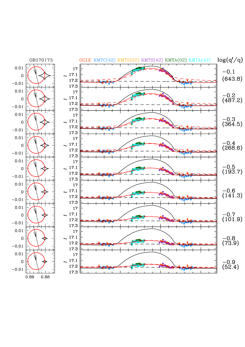
Figure 5: Nine simulations of OGLE-2017-BLG-0173 (von Schlieffen solution A), similar to Figure 4. The values in parentheses are $\Delta\chi^{2}=\chi^{2}({\rm 1L2S})-\chi^{2}({\rm 2L1S})$, by which binary source models are excluded. To the eye, the degeneracy between these solutions and those in Figure 6 (Cannae solution B) persist at all $q$.

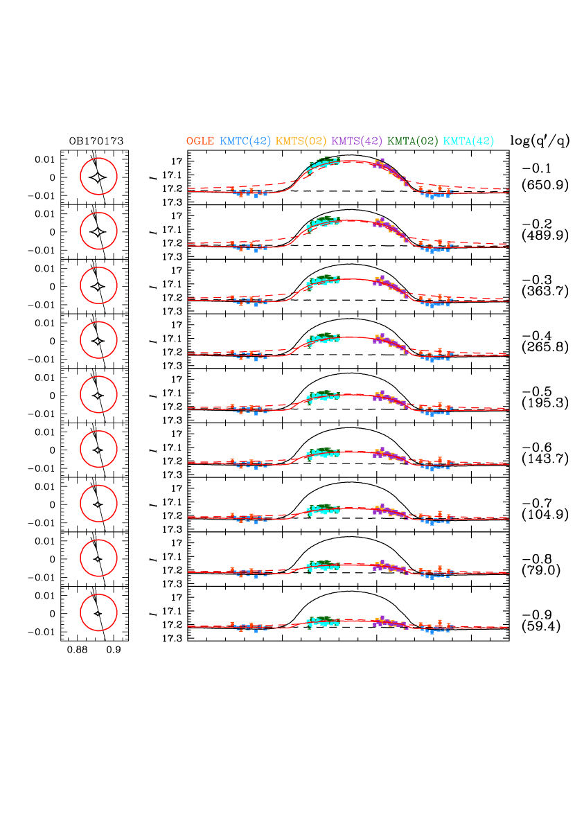
Figure 6: Nine simulations of OGLE-2017-BLG-0173 (Cannae solution B), similar to Figure 4. The values in parentheses are $\Delta\chi^{2}=\chi^{2}({\rm 1L2S})-\chi^{2}({\rm 2L1S})$, by which binary source models are excluded. To the eye, the degeneracy between these solutions and those in Figure 6 (von Schlieffen solution A) persist at all $q$.

As shown in their Figure 1, the event betrays no hint of an anomaly in OGLE data, so the decision to examine quick-look KMTNet data was not influenced in any way by the presence of a planet. Thus, we must evaluate the minimum value of $q$ that would have triggered a decision to re-reduce the data and then determine whether the resulting light curve would have been reliable enough to warrant publication of the (putative) planet. We note that, as shown in their Figure 3, the “bump” in the KMTNet data was caused by the edge of a large source grazing the center of the caustic for solution (A) and by the center of a large source passing directly over the caustic for solution (B). Figures 5 and 6 show sets of nine simulated light curves for $\log(q^{\prime}/q)=-0.1,-0.2,\ldots-0.9$, for solutions A and B, respectively. The first point is that to the eye, the two figures look identical, except that the geometries at the left are quite distinct. Second, one sees that within each figure, the bump looks qualitatively similar in all cases, which is fundamentally due to the “Hollywood” (Gould, 1997; Hwang et al., 2018) character of the event. The main difference is that the height of the bump scales $\propto q$ (as discussed by Hwang et al. 2018; see their Equations (9) and (10)). We estimate that at $\log(q^{\prime}/q)=-0.7$ the “bump” (now 0.06 mag, compared to the actual one of 0.3 mag), would have still triggered a further investigation for either solution A or B. Further, the numbers at the right show $\Delta\chi^{2}=\chi^{2}({\rm 1L2S})-\chi^{2}({\rm 2L1S})$ between binary-source (1L2S) and binary-lens (2L1S) models. These values are certainly high enough to exclude the 1L2S interpretation.

However, we find that at $\log(q^{\prime}/q)=-0.7$, and indeed at all $q^{\prime}$ shown in the figures, the analysis of either simulated data set (A or B) yields a discrete degeneracy between the two classes of models (von Schlieffen and Cannae), with $\Delta\chi^{2}<10$ and $\Delta\log q>0.3$ between the two minima. That is, they all suffer from essentially the same degeneracy as the original event. Hence, although for $\log(q^{\prime}/q)\geq-0.7$, we judge that they all would have been published (just as the original event was, Hwang et al. 2018), they all would have been excluded from the analysis.

This exclusion has no practical importance from the perspective of the present mass-ratio-function analysis, because the original event is itself excluded. However, the persistence of this degeneracy is of significant interest. Hwang et al. (2018) had noted that the other published Hollywood event, OGLE-2005-BLG-390 (Beaulieu et al., 2006), did not suffer from this von Schlieffen/Cannae degeneracy. And they further noted that the caustic was much smaller than the source in that case, whereas the caustic was of comparable size to the source for OGLE-2017-BLG-0173. They therefore conjectured that the degeneracy was a consequence of the caustic size relative to the source size. However, the present analysis shows that this is clearly not the case. Hence, there must be some other governing factor. This may be the angle of the source trajectory, $\alpha$, but investigation of this question is well outside the scope of the present work.

6.1.3 OGLE-2016-BLG-1195

OGLE-2016-BLG-1195 was analyzed by two groups (Bond et al., 2017; Shvartzvald et al., 2017) based on completely different data sets. The two groups obtained slightly different mass-ratio estimates $q=4.22\pm 0.65\times 10^{-5}$ (Bond et al., 2017) and $q=5.60\pm 0.75\times 10^{-5}$ (Shvartzvald et al., 2017). Here we adopt a weighted average $q=4.81\pm 0.49\times 10^{-5}$.

The anomaly in this event was discovered and publicly announced by the MOA collaboration in real time, i.e., at UT 15:45 29 June. In fact, while the internal discussions that led to this alert were still ongoing, the MOA observers increased the cadence of observations, beginning at UT 15:15. That is, prior to this change, MOA observed the field steadily at a cadence of $\Gamma=4.0\,{\rm hr}^{-1}$, which is their normal cadence for this field, whereas between UT 15:15 and UT 16:48 (roughly the “end” of the anomaly), the field was observed 16 times, for a mean cadence of $\langle\Gamma\rangle=10.3\,{\rm hr}^{-1}$. A slightly lower cadence continued for the rest of the night. See Bond et al. (2017).

Hence, in contrast to the previous two cases, one must consider two possible data streams for any mass ratio $q^{\prime}$: the actual one (in the case that the observers would have recognized the anomaly and so taken the initiative to increase the cadence) and one in which the anomaly was not recognized, so the cadence remained at the standard $\Gamma=4.0\,{\rm hr}^{-1}$. Fortunately, as we show below, the two cases lead to very similar conclusions. This is partly because the anomaly had already peaked when the cadence was changed and partly that there existed an independent data set from KMTA.

We first focus on the more conservative case, i.e., that at sufficiently low $q^{\prime}$, the observers would not have recognized the anomaly. This leads us to construct a “thinned” version of the MOA online data set that is consistent with the normal MOA cadence. For the times that MOA observed the field two, three or four times consecutively (in 1.5 min intervals), we always choose the second of these observations. For the remaining observations, we thin them so that the surviving observations are as closely spaced to 15 minutes as possible. In particular, we keep six observations from the 16 observations during the final 93 minutes of the anomaly.

Then, under either assumption (real-time anomaly recognition or not), and as for the two other events previously examined, we address two questions, whether the anomaly would ultimately have been recognized and, if so, whether the re-reduced data would have yielded a reliable planet detection. A very important difference from the previous two cases, however, is that the full extent of the anomaly was continuously observed by two different surveys, MOA (Bond et al., 2017) and KMTA (Shvartzvald et al., 2017), from sites separated by several thousand km. The data quality was overall roughly comparable (judged by the quoted errors of parameters). Hence, the normal caution that a low-amplitude signal might be due to unknown systematics would not apply to this case, since the same signal would be present in both data sets. Moreover, even though the actual analyses were done in two separate papers, a joint paper combining both data sets would have been written if neither data set was by itself adequate for publication.

As noted above, the first threshold is simply recognizing the anomaly. This need not have been in real time. In principle, it could have been recognized later in either the MOA or KMTNet data. However, in contrast to the two cases discussed above, the 2016 quick-look KMTNet data were of substantially lower quality, and tests show that the anomaly would not have been recognized according to the procedures followed in that year. Hence we should examine only the on-line MOA data. We note that the event was a Spitzer microlensing target (Shvartzvald et al., 2017), part of a broader program to measure the Galactic distribution of planets (Gould et al., 2015a, b; Yee et al., 2015; Calchi Novati et al., 2015; Zhu et al., 2017), and therefore the MOA data would have been examined quite closely even if the anomaly had not been detected in real time.

Following the above considerations, we examined fake light curves constructed on the basis of MOA online data, both with and without the additional MOA points triggered by the alert. We are confident that the anomaly would have triggered re-reductions of MOA and KMTNet data for $\log(q^{\prime}/q)=-0.3$ and perhaps even lower. However, we do not investigate the exact threshold, nor do we show the plots that we reviewed because, as we now describe, the fundamental issue is not simply recognizing that there was an anomaly.

Figure 7 shows 9 panels with $\log(q^{\prime}/q)=-0.05,-0.10,\ldots-0.45$, with re-reduced data from both MOA and KMTA. In each panel, we show both the planetary (2L1S) and binary source (1L2S) models. The number in parentheses to the right of each panel gives the $\Delta\chi^{2}\equiv\chi^{2}({\rm 1L2S})-\chi^{2}({\rm 2L1S})$ difference between these models. For $\log(q^{\prime}/q)=-0.30$, $-0.35$, and $-0.40$, these are 17.6, 13.6, and 9.7 respectively. Given that two independent data sets are contributing to these values and that neither shows any sign of systematics, we conclude that the first two would be considered adequate for a reliable detection of a planet, while the third would not.

Next, we address the role of the real time alert. If the event were not recognized in real time at lower mass ratio (as it was in the actual case) then the only difference in the evaluation of publishability would be the “exclusion” of $\sim 10$ MOA points during the second half of the anomaly (plus some post-anomaly points), which would imply slightly lower $\Delta\chi^{2}$. In particular, for $\log(q^{\prime}/q)=-0.30$ and $-0.35$, $\Delta\chi^{2}=13.1$ and 10.2, respectively. By the argument just given, these would render the first as a publishable planet and the second not. Hence, the only relevant question about real-time alerts is whether, at $\log(q^{\prime}/q)=-0.35$, the event would have been alerted based on the online MOA data. Given that the actual event was not recognized by the observers until the deviation was nearly at peak, and so with roughly twice the deviation as the $\log(q^{\prime}/q)=-0.35$ case, we regard this as highly unlikely. Thus, we conclude that the threshold for detection/publication is $\log(q^{\prime}/q)=-0.30$.

Finally, we analyze the simulated $\log(q^{\prime}/q)=-0.30$ as though it were a real event. We find that there is a unique minimum and that $\sigma(\log(q))=0.10$. Hence, it clearly meets our criterion (2).

6.1.4 OGLE-2013-BLG-0341

OGLE-2013-BLG-0341 was originally recognized as having a minor-image planetary anomaly at HJD${}^{\prime}=6393.7$ based on real-time OGLE data, four days after the anomaly, when A.G. cataloged it as a possible high magnification event and therefore carefully examined the light curve as part of his assessment. He publicly announced this but also noted that since the lower limit on the magnification, $A_{\rm max}>10$, was not particularly high, no immediate action was warranted. However, from this point on, the event was closely monitored with the aim of organizing intensive followup observations near peak, if indeed its prospective high-mag character was confirmed. Such intensive observations were in fact initiated 10 days after the anomaly and about two days before peak. The peak was characterized primarily by a binary (not planetary) caustic. However, Gould et al. (2014) later showed that the planet’s parameters could be recovered even when the data points in the vicinity of the planetary anomaly (144 points. to be precise) were removed from the data.

The initial recognition of the planetary dip can be partially attributed to chance. The purpose of A.G.’s review of the online OGLE light curves was not to find planetary anomalies, but rather high-magnification events that could be intensively monitored to find planets near peak (Gould et al., 2010). Thus, it was hardly guaranteed that the actual signal would have been noticed when it was, and it is fairly unlikely that it would have been noticed at this point if the dip had been only half as deep.

Nevertheless, because the event eventually did become high-magnification, the light curve would have been singled out for extremely close inspection, regardless of whether a planetary anomaly had previously been noticed or not. If the planet had been noticed at this point, then of course exactly the same followup observations would have been initiated. If not, then when the event showed very obvious binary-like behavior (see Figure 1 of Gould et al. 2014), the event would have been abandoned as “not interesting”. Hence, the signature from the planet in the caustic exit would have been drastically reduced due to lack of follow-up data.

In brief, an important (though as we shall see, not only) question of whether the planet would have been recognized comes down to: would Gould et al. (2014) have recognized the planetary signature once they began closely examining this high-mag event, as it approached peak?

Figure 8 shows nine panels with $\log(q^{\prime}/q)=-0.05,-0.10,-0.15,-0.2,-0.3,-0.4,-0.5,-0.75,-1$. This event is unique in our sample in that as $q$ declines, the anomaly becomes less visible and then invisible, but then begins to become more visible again at $\log(q^{\prime}/q)=-0.3$. Then, at $\log(q^{\prime}/q)=-0.5$, its visibility peaks, whereupon it gradually declines. The reason for this behavior is that in the actual event, the source passed along the trough between the two triangular, minor-image caustics, but very close to one of the caustic walls. The source trajectory relative to the mid-line of the trough remains basically the same as $q$ declines, but because the triangular caustics move closer together, the edge of the source moves increasingly over the caustic wall. At first, the excess magnification of the limb increasingly cancels the dip due to the main part of the source passing through the trough. However, when $q$ falls sufficiently, the excess magnification starts to dominate, and there is a bump in place of the trough.

The scatter in the OGLE online data for the six points on the night of the anomaly is small, $\sigma=0.03\,$mag. Hence, a mean deviation of just 0.06 mag would be a five-sigma detection, which we regard as the minimum needed to be both recognizable by eye and to engender sufficient confidence to trigger a massive followup campaign, as discussed above. This threshold has already been crossed at $\log(q^{\prime}/q)=-0.15$ for the “fading” dip. It is crossed again for the “rising” bump at $\log(q^{\prime}/q)=-0.3$ and then is crossed again for the “fading” bump slightly below $\log(q^{\prime}/q)=-0.75$. We conclude that followup observations would have been triggered in the two ranges $(\log(q^{\prime}/q)>-0.1)$ and $(-0.3>\log(q^{\prime}/q)>-0.75)$.

Nevertheless, we now argue that only in the former range would a paper claiming secure detection of a planet have been written. First, in contrast to a dip in the light curve (which can only be explained by a minor-image anomaly), an isolated bump in the light curve can also be explained by a 1L2S solution. The OGLE anomaly data are confined to a narrow range in time, and so have no leverage on the shape of the bump to distinguish between 2L1S and 1L2S.

In principle, the followup data (which we argued above would have been triggered for the second – “bump” – range of $q$) could have confirmed the planetary nature of the anomaly. However, there are two practical issues that severely undermine this possibility. First, at our finally adopted value of $\log(q^{\prime}/q)\leq-0.1$, we find that this confirmation is already relatively weak, $\Delta\chi^{2}=66$, a point to which we return below. More fundamentally, it is very unlikely that the analysis would have been pushed to the point that the test would have been devised of deleting the planetary-anomaly data. The analysis of the event was quite complex and required enormous human and computer resources. It was only in the process of carrying out this analysis that it was discovered that such confirmation was possible. Hence, the motivation to analyze an event to this level in the case that there was a (seemingly) unassailable non-planetary interpretation would almost certainly have been lacking. Finally, even supposing that such an analysis were done, the “confirmation” of $\Delta\chi^{2}<50$ would almost certainly not have been regarded as sufficient to claim a secure detection. This is reflected in the fact that Gould et al. (2014) specifically argued that the unambiguous planetary anomaly (due to the fact that it was a minor-image dip) served as “confirmation” that the subtle – and by eye, invisible – deviations in the binary caustic could be regarded as a reliable indicator of a planet. Without such independent knowledge, and at relatively low $\Delta\chi^{2}$, this would have at best led to the reporting of an interesting planetary candidate.

We conclude that the threshold for planet detection is $\log(q^{\prime}/q)=-0.10$. We confirm that this solution is unique and find $\sigma(\log(q))=0.04$, implying that our sample criteria are satisfied at this threshold.

6.1.5 MOA-2009-BLG-266

MOA-2009-BLG-266 (Muraki et al., 2011) was recognized as having a potentially planetary anomaly in real time by the MOA collaboration at the end of the New Zealand night from the sharp decline in the previously smoothly rising light curve. This triggered follow up observations at many sites, which further articulated the decline, mapped the trough and then the rise. The basic model of the event was already derived before any of these followup data were taken, let alone reduced, so that in the actual case, the alert-generated data were needed for full characterization of the planet, but not for its discovery. However, if the mass-ratio had been lower, it is possible that the planet could not have been characterized well enough to warrant publication in the absence of the followup data. Thus, for this event, it is especially important to evaluate both how well the planetary perturbation could have been recognized in real time, and how well the planet could have been characterized with, and without, followup observations.

We note that five different observatories took data on MOA-2009-BLG-266 prior to the alert, of which four also took data after the alert. Hence, one must assess whether these four would have taken data in the absence of the alert. We find that only one of these (Canopus) took data in a way that indicated sustained focus on the event as it approached peak: they took four points spread over 1.4 hours on the night before the alert. The others either took one point on occasional nights or had stopped taking data altogether. Thus, it is reasonable to suppose that Canopus would have also taken four points on the next night, even if there had been no alert. However, these data would have overlapped MOA data and so would not have qualitatively altered how well the event could have been characterized in the absence of an alert (and so absence of data in the trough).

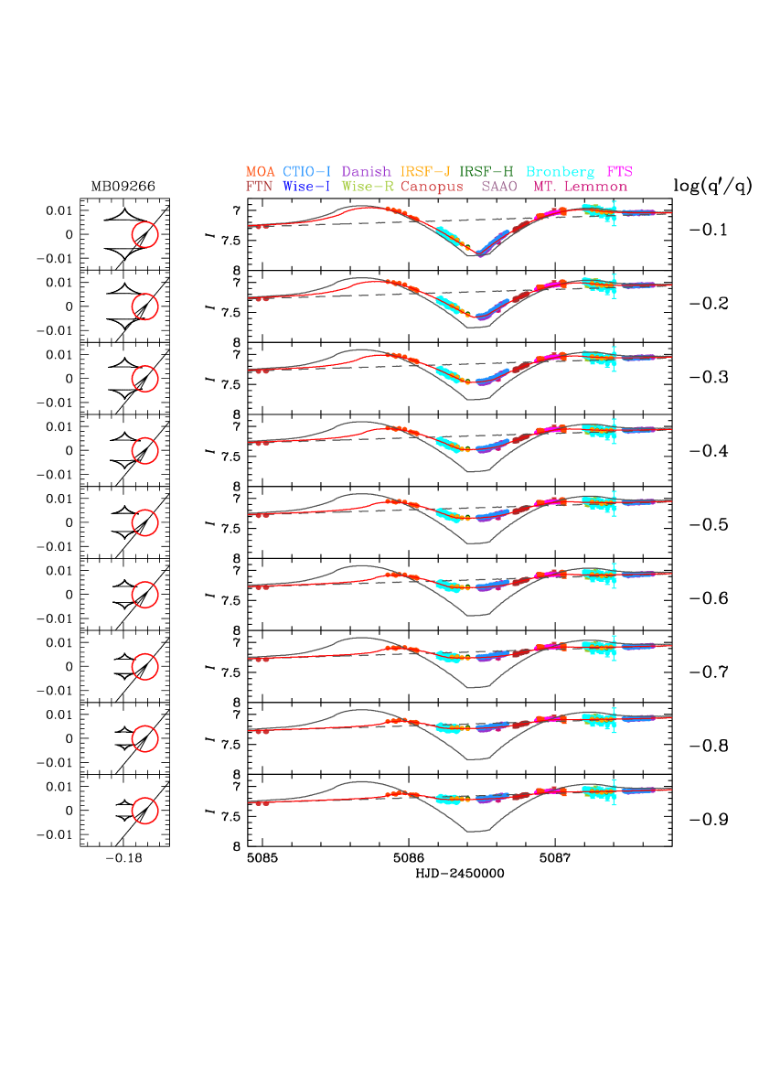
Figure 9: Nine simulations of MOA-2009-BLG-266, similar to Figure 4. The simulations are based on re-reduced data from all observatories.

Figure 9 shows nine panels with $\log(q^{\prime}/q)=-0.1,-0.2,\ldots-0.9$ and all data re-reduced. The first question is whether, with a smaller mass ratio, MOA would have issued an alert (based, of course, on online data). While Figure 9 shows re-reduced data, it still enables us to understand how the basic form of the MOA light curve evolves as $q$ declines: over the range $\log(q^{\prime}/q)\leq-0.6$, it basically takes the form of a mean excess over the point-lens model (dashed line). We now argue that an anomaly of this form would give rise to an alert provided that the mean excess over the predicted point-lens light curve was 0.1 mag.

Based on the MOA online data from before the night of the anomaly, we find that one can predict the flux (based on a point-lens model) on the night of the anomaly to 0.085 mag at $3\,\sigma$ confidence. There are 10 MOA points on that night, with scatter 0.024 mag. Hence a standard error of the mean of 0.008 mag. Thus, a mean offset of 0.1 mag would yield a $\Delta\chi^{2}\sim 12$ discrepancy, which would be sufficient indication to issue an alert. This condition is satisfied for $\log(q^{\prime}/q)=-0.6$, but not lower mass ratios. At higher mass ratios, the mean offset itself satisfies this condition, and in addition there is increasing evidence of a decline (which is what triggered the actual alert).

We fit simulated data for the case $\log(q^{\prime}/q)=-0.6$, and find that the solution is both unique and well localized ($\sigma(log(q))=0.02$). We then repeat this exercise for $\log(q^{\prime}/q)=-0.7$ but with only MOA and Canopus data (since, as we argued above, there would be no alert and hence no followup data apart from Canopus). We find that there are several local minima from the broad search of parameter space, and that none of the models derived at these minima appear compelling enough to warrant publication.

We conclude that the threshold for this event is $\log(q^{\prime}/q)=-0.6$.

6.1.6 OGLE-2007-BLG-368

The details of the anomaly alert of OGLE-2007-BLG-368 are recounted by Sumi et al. (2010). The first alert was given by the robotic SIGNALMEN anomaly detector (Dominik et al., 2007) JD${}^{\prime}=4302.314$, being triggered by the nine MOA points that lie $\sim 0.2\,$mag below the point-lens model. This alert prompted followup observations beginning 5 hours later in Chile by the $\mu$FUN SMARTS 1.3m telescope and the PLANET Danish 1.5m, and then from additional telescopes continuing toward the west. From the present perspective, it is important to note that this alert did not reach the MOA observer and so did not influence the cadence of MOA observations on the night HJD${}^{\prime}\sim 4303$. These were the next observations after those in Chile. Hence, the next observations that were influenced by the alert (after Chile) were from the PLANET Canopus observations from Tasmania, whose three closely spaced points basically overlap the last MOA point. There were additional followup observations, which played an important role in characterizing the actual event, but as we will show, these play very little role in the current $V/V_{\rm max}$ analysis.

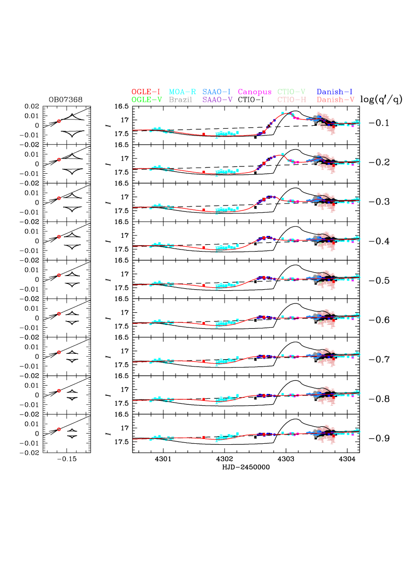
Figure 10: Nine simulations of OGLE-2007-BLG-368, similar to Figure 4. This figure is based on re-reduced data from all observatories. It should be compared to the next one (Figure 11), which is based on “online” OGLE and MOA data.

Figure 10 shows nine panels with $\log(q^{\prime}/q)=-0.1,-0.2,\ldots-0.9$ and all data re-reduced. Note that for $\log(q^{\prime}/q)\leq-0.4$, the point-lens model and the planetary model are nearly identical for the followup data taken HJD${}^{\prime}>4303.3$. That is, only the $\mu$FUN Chile, Danish Chile, and Canopus data would have played a significant role for $\log(q^{\prime}/q)\leq-0.4$.

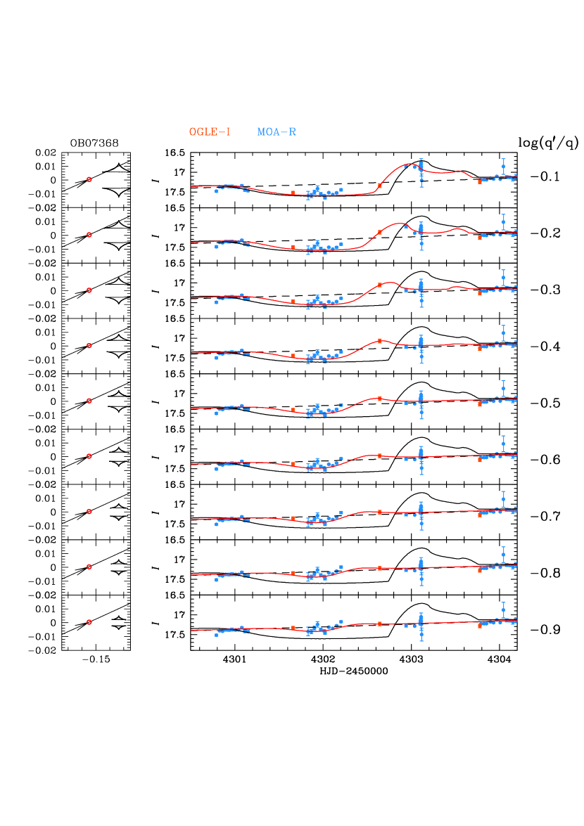
Figure 11: Nine simulations of OGLE-2007-BLG-368, similar to Figure 4. This figure is based on “online” OGLE and MOA data. It should be compared to the previous one (Figure 10), which is based on re-reduced data from all observatories.

Figure 11 shows the same nine panels as Figure 10 but with only online survey data. Based on this figure, we consider it to be unlikely that there would have been an alert on this event in time to trigger CTIO observations for $\log(q^{\prime}/q)\leq-0.4$. Moreover, we can say with near certainty (since A.G. made this decision) that CTIO would not have responded to such an alert if it had been given. However, the CTIO response is of secondary importance because the Danish data, which cover the same time interval, would certainly have been taken.

As usual, we first ask at what threshold would the online survey data have led to re-reductions, and then ask whether these reductions would have led to a publishable result given the data that would have been acquired.

The online OGLE data would, by themselves, certainly have triggered re-reductions at $\log(q^{\prime}/q)\geq-0.4$. At $\log(q^{\prime}/q)=-0.5$ this is less probable, but in this case the partial corroboration from online MOA data would have almost certainly led to re-reductions. Re-reduction at $\log(q^{\prime}/q)=-0.6$ is also a possibility.

Recall that at $\log(q^{\prime}/q)=-0.3$, we concluded that there would have been an anomaly alert. We analyze all data and find that the solution is well-localized with $\sigma(\log q)=0.025$. At $\log(q^{\prime}/q)=-0.4$, we must consider two cases, i.e., with and without the alert (and so followup data). We find that with the followup data, the minimum is well localized with $\sigma(\log q)=0.08$, so satisfying all our criteria. However, with survey-only (re-reduced) data, we find that there are two minima separated by $\Delta\chi^{2}<10$ and $\Delta\log q>0.3$, which would fail our third criterion. Since we assessed that there would probably not be an alert at $\log(q^{\prime}/q)=-0.4$, we conclude that the threshold for detection is $\log(q^{\prime}/q)=-0.3$. We recognize that there is some probability of an alert at $\log(q^{\prime}/q)=-0.4$, and therefore (according to the analysis just given) of a publishable detection. However, since we are approximating probabilities $P$ as either zero or one, we simply adopt the threshold $\log(q^{\prime}/q)=-0.3$.

6.1.7 OGLE-2005-BLG-390

OGLE-2005-BLG-390 was detected primarily in follow-up data organized by the PLANET collaboration, but in contrast to all previous cases, all of these data were taken in response to an alert of the microlensing event itself, not an anomaly (Beaulieu et al., 2006). The anomalous behavior was noted by the observer at the Danish telescope in Chile, and in principle this could have influenced other observatories farther to the west, but a detailed investigation at the time showed that this was not the case. Hence, the same observations would have been taken over the anomaly whether a planetary signal was suspected to be present or not.

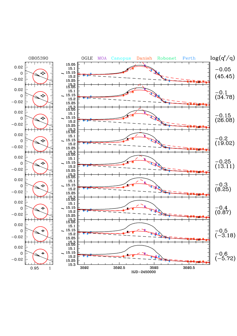
Figure 12: Nine simulations of OGLE-2005-BLG-390, similar to Figure 4. It is based on re-reduced data from all observatories, since these reductions would have been carried out whether or not a planet was suspected.

Figure 12 shows nine panels with $\log(q^{\prime}/q)=-0.05,-0.10,\ldots,-0.30,-0.40,-0.50,-0.60$ and all data re-reduced. This event was one of relatively few monitored by the PLANET collaboration, and hence the data would have been very closely inspected even if the anomaly had not been noticed in real time. Thus, the anomaly would have been easily noticed at $\log(q^{\prime}/q)=-0.5$ and probably somewhat below. However, as we now show, it is not important to evaluate the exact boundary of this recognition.

Because the anomaly is a smooth bump, it can potentially be fit as a binary source event, 1L2S. In the actual event, this degeneracy was investigated and ruled out both by $\Delta\chi^{2}=46$ and also by obvious deviations in the light curve from the 1L2S model. However, for $\log(q^{\prime}/q)=-0.25$, we see that 2L1S is favored over 1L2S by only $\Delta\chi^{2}=13$. For the case of OGLE-2016-BLG-1195, we regarded this value as marginally acceptable because there were two independent data sets that spanned the entire anomaly. However, in the present case, which lacks such confirmation, we regard it to be marginally unacceptable and therefore adopt a threshold of $\log(q^{\prime}/q)=-0.2$. We find that at this threshold, $\sigma(\log q)=0.11$, which satisfies our sample criterion $\sigma(\log q)<0.15$.

6.1.8 OGLE-2005-BLG-169

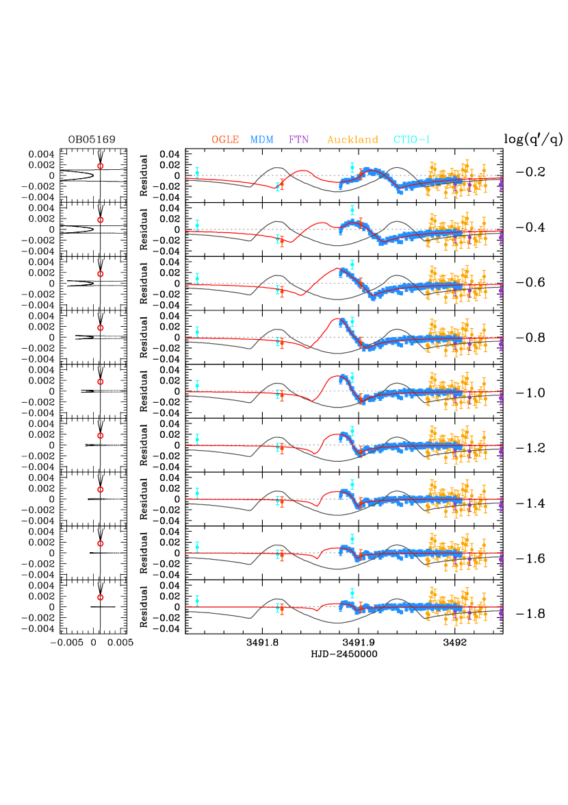
Figure 13: Nine simulations of OGLE-2005-BLG-169, similar to Figure 4. It is based on re-reduced data from all observatories, since these reductions would have been carried out whether or not a planet was suspected.

The overwhelming majority of evidence for a planet in the OGLE-2005-BLG-169 data lies in the extremely intensive followup data taken from the MDM observatory in Arizona, beginning very close to the peak of the event (Gould et al., 2006). As with all data in and near the anomaly of this event (and like OGLE-2005-BLG-390), these were obtained without reference to the possible existence of a planet. Because the dense data began near peak, there was a modest ambiguity in the solutions presented by Gould et al. (2006). This was resolved by the analyses of Bennett et al. (2015) and Batista et al. (2015) when they, respectively, partially and fully resolved the lens 6.5 and 8.2 years after the event. Here we use their parameters for the event, in particular $q=6.1\times 10^{-5}$. Figure 13 shows nine panels with $\log(q^{\prime}/q)=-0.2,-0.4,\ldots-1.8$, with all data re-reduced.

Because of the unprecedented character of the data set, roughly 1000 high-precision data points (later binned to 137) taken over three hours, the data were examined extremely closely. Although the deviation from a point lens was noticed very quickly, submission of the manuscript was delayed for 10 months, primarily because of concerns that the quite small amplitude of the deviations might be due to variable weather conditions, which were very severe during the night of the anomaly. In the end, the decision to publish was based on the unambiguous discontinuous change of slope at HJD${}^{\prime}=3491.97$. Such discontinuities are a generic feature of microlensing caustic crossings but would be extremely difficult to produce by weather-induced artifacts.

Using the same criteria (and relying on the judgment of A.G., who made the original decision to publish) we conclude that the simulation with $\log(q^{\prime}/q)=-1.2$ would marginally meet this condition. We fit simulated data at this value and find that $\sigma(\log q)=0.174$, which does not satisfy our sample criterion. However, at $\log(q^{\prime}/q)=-1.0$, we find $\sigma(\log q)=0.10$, and so adopt $\log(q^{\prime}/q)=-1.0$ as our threshold.

6.2 Constraints of the Mass-Ratio Function $F(q)$

If $F(q)$ is chosen correctly, then we expect the seven $r_{i}$ defined by Equation (10) to be uniformly distributed on the interval [0,1]. As discussed in the separate analyses of each event in Section 6.1 (and in particular, in Section 6.1.4), in all cases $P_{i}$ takes the form $P_{i}(q^{\prime})=\Theta(10^{-4}-q)\Theta(q-q_{{\rm min},i})$, where $\Theta$ is a Heaviside step function and $q_{{\rm min},i}$ has been evaluated separately for each event. Hence Equation (10) reduces to Equation (11)

We expect then that

$${1\over N}\sum_{i=1}^{N}r_{i}={1\over 2}\pm(12N)^{-1/2}\longrightarrow 0.500\pm 0.109,$$ (12)

where $N=7$. We also expect that the distribution of $r_{i}$ will be consistent with uniform based on a Kolmogorov-Smirnov (KS) test. To take an extreme example, if for a given trial function $F(q)$, each of the $r_{i}$ were exactly equal to 0.58, then Equation (12) would be satisfied, but the distribution would not be consistent with uniform $(p<1\%)$. Nevertheless, since KS is a relatively weak test, it would be surprising if a function that satisfied Equation (12) did not meet this second criterion as well.

We begin by considering power laws $F(q)\propto q^{p}$. Applying Equation (12), we find that

$$p=1.05^{+0.78}_{-0.68}\qquad\rm(this\ work).$$ (13)

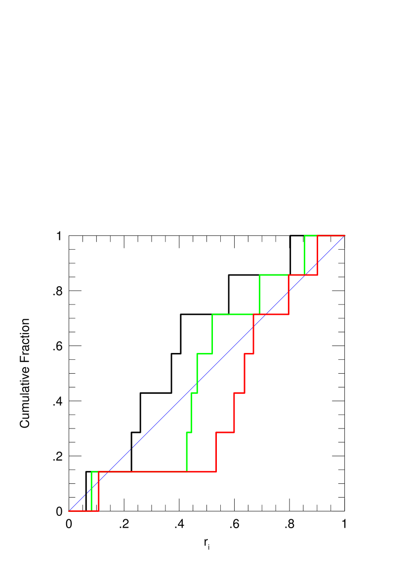
Figure 14: Cumulative distribution of the “$V/V_{\rm max}$” parameter $r_{i}$ defined by Equations (10) and (11) for three power laws $dN/d\ln q\propto q^{p}$, where $q$ is the mass ratio and $p=1.05$ (green), $p=0.37$ (black), and $p=1.83$ (red). These represent the best fit and $1\,\sigma$ lower and upper limits, respectively. In all cases, a Kolmogorov-Smirnov test shows that these are consistent with being drawn from a uniform distribution. Hence, there is no basis to reject a power-law for the mass-ratio function from this analysis. The best fit value confirms a sharp turnover in the mass-ratio function relative to that found by Sumi et al. (2010) and Suzuki et al. (2016) at higher mass ratios.

Figure 14 shows the cumulative distribution at the best fit and $1\,\sigma$ limits displayed in Equation (13). These have maximal differences (relative to uniform) of $D=(0.285,0.309,0.391)$ with corresponding KS $p$-values $p=(0.53,0.43,0.18)$. That is, there is no independent information from the uniformity (or lack of it) that would indicate that any of these functions is unacceptable at the $1\,\sigma$ level. Therefore, there is also no basis for rejecting a power-law form for the distribution in the domain probed by our sample.

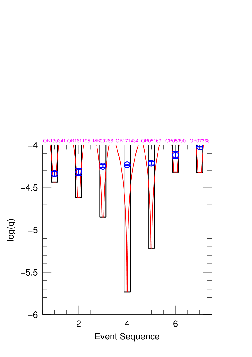
Figure 15: Illustration of the “$V/V_{\rm max}$” method. The blue circles show the best fit $q$ from the actual event, while the bottoms of the black rectangles show the lowest $q^{\prime}$ that could have been detected. The red curves show the relative frequency of different mass ratios according to the best-fit power law, $dN/d\ln q\propto q^{1.05}$. These can be compared to the relative frequencies that would be expected from a hypothetical law $dN/d\ln q=$const (black). If the frequency function is chosen correctly, then on average, half of the red “volume” should be above the blue points. More generally, the ratio $r_{i}$ of this “volume” to the total “volume” should be consistent with being uniformly distributed over the interval [0,1].

Figure 15 illustrates the “$V/V_{\rm max}$” method as well as the best fit result. For each event (listed at the top), the observed mass ratio $q$ is shown by a blue point, while the lowest $q^{\prime}$ at which it could have been detected is shown by the bottom of the rectangular box. The boxes themselves have uniform width, which illustrates the relative frequency of $q^{\prime}$ values for the hypothetical case $dN/d\ln q\propto q^{0}={\rm const}$, i.e., $p=0$. The red curves show the relative frequency for the best-fit case, $p=1.05$. The parameter $r_{i}$ is the ratio of the volume “$V$” (i.e., area) contained within the red curve above the actual detection, divided by the total volume “$V_{\rm max}$” within the red curve. The best-fit value ($p=1.05$), illustrated in the figure, occurs when $\langle r_{i}\rangle=0.5$.

Equation (13) is consistent with the results of Suzuki et al. (2016), who found $p=0.6^{+0.5}_{-0.4}$ based on an almost completely independent argument. Since these arguments are essentially independent, we can combine the two measurements (weighted according to the quoted errors) to obtain

$$p=0.73^{+0.42}_{-0.34}\qquad\rm(this\ work\ +\ Suzuki\ et\ al.\ 2016)$$ (14)

6.3 $\Delta\chi^{2}$ at Threshold

In contrast to the present investigation, all previous microlensing studies of the planet mass or mass-ratio function have used a detection-efficiency analysis, which compares the detected planets to a calculation of the overall planet sensitivity of the sample. The vast majority of these analyses calculate the planet sensitivity either by fitting planetary models to the data following Gaudi & Sackett (2000) or by simulating light curves with planets following Rhie et al. (2000). In both cases, the “detectability” of a given planet is assessed relative to a fixed $\Delta\chi^{2}$ threshold comparing 1L1S models to 2L1S. Early analyses used $\Delta\chi^{2}=60$ as their detection threshold (Albrow et al., 2001; Gaudi et al., 2002), but other studies have used thresholds ranging from $\Delta\chi^{2}=60$ to $\Delta\chi^{2}=500$ (Sumi et al., 2010; Gould et al., 2010; Cassan et al., 2012; Suzuki et al., 2016). In the analysis of individual events, different authors have used different thresholds depending on the exact event and on whether or not the planet signal comes from a central caustic or a planetary caustic (e.g., Section 8 of Sumi et al. 2010 and references therein). For example, Yee et al. (2013) argued based on the analysis of MOA-2010-BLG-311 that $\Delta\chi^{2}\sim 80$ is insufficient to claim a secure planet detection, even though this is above the $\Delta\chi^{2}$ threshold used in many studies. They also suggested that this event is evidence that the threshold for high-magnification/central-caustic crossing perturbations may be higher than for planetary caustic perturbations.

Although the $V/V_{\rm max}$ analysis presented here was designed to answer a different question, we can use the results of this analysis to explore $\Delta\chi^{2}$ at the threshold of planet detection. Table LABEL:tab:chi2 shows $\Delta\chi^{2}\equiv\chi^{2}$(1L1S)$-\chi^{2}$(2L1S) [or $\chi^{2}$(2L1S)$-\chi^{2}$(3L1S) in the case of OGLE-2013-BLG-0341] at our adopted threshold of “publishability” for the eight events considered here (including two models for OGLE-2017-BLG-0173). The most striking feature of this table is that $\Delta\chi^{2}$ at threshold spans a factor of 100. As we discuss below, the extreme broadness of this range is partly due to the heterogeneous character of the sample. However, even after accounting for this heterogeneity, Table LABEL:tab:chi2 strongly suggests that $\Delta\chi^{2}$ is a relatively poor proxy for “publishability”. Before we begin this review, we emphasize that we regard “publishability” as a more appropriate criterion that “detectability” because anomalies can be “detectable” and unambiguously real, yet still be uninterpretable at a level that is scientifically interesting.

The four events for which the threshold was $\Delta\chi^{2}<500$ shed the most light on this question: OGLE-2005-BLG-169, OGLE-2016-BLG-1195, OGLE-2013-BLG-0341, and OGLE-2005-BLG-390, with $\Delta\chi^{2}=184$, 257, 309, and 457, respectively. These are naturally grouped into two pairs: OGLE-2005-BLG-169 and OGLE-2013-BLG-0341 were both identified from very short features whose signatures were unambiguously planetary, while for both OGLE-2016-BLG-1195 and OGLE-2005-BLG-390, the threshold was set by confusion with 1L2S models.

As discussed in Section 6.1.8, the actual decision to publish OGLE-2005-BLG-169 was based on the secure recognition of a discontinuity in the slope of the light curve. Such discontinuities cannot be produced by any microlensing effect other than a planetary (or binary) companion and would be extremely difficult to generate by instrumental or weather problems. We found in Section 6.1.8 that at the threshold of “by-eye confidence” in the reality of this feature, the mass-ratio error $\sigma(\log q)=0.10$ is relatively close to our adopted threshold of $\sigma(\log q)<0.15$. Thus, by two independent modes of assessment, this event would have been “barely publishable” at the adopted threshold.

For OGLE-2013-BLG-0341, the key signature was an isolated dip, which can only be produced by a minor-image perturbation. Moreover, such short-lived dips can only be produced by planets. While the total $\Delta\chi^{2}$ of the planet is higher than that of OGLE-2005-BLG-169 by 125, this difference is somewhat deceptive. Recall from Section 6.1.4 that $\Delta\chi^{2}($binary-caustic$)=66$ came from the perturbation induced by the binary caustic. However, this binary-caustic “confirmation” played no role in our assessment of whether the planet would have been published at the adopted threshold. Hence, if the system had been a simple 2L1S system, or if the trajectory happened to miss the central caustic, the decision would have been exactly the same. In these cases, $\Delta\chi^{2}=309-66=243$. Moreover, we have not attempted to assess the exact $\log q^{\prime}/q$ at which the event would have ceased to be publishable, mainly because this level of precision would not contribute significantly to our study, but also because we do not believe that such precision is feasible. Hence, these two values (184 and 243) for these two “short timescale feature” events should be regarded as comparable.

In brief, based on this admittedly small sample of two, it appears feasible to publish “short timescale feature” events with $\Delta\chi^{2}\gtrsim 200$.

It is quite notable that the two events whose threshold is set by confusion with 1L2S models have substantially different $\Delta\chi^{2}$ in Table LABEL:tab:chi2, i.e., 257 versus 457. It is true OGLE-2005-BLG-390 was subjected to a slightly stronger $\Delta\chi^{2}$ threshold to reject 1L2S ($\Delta\chi^{2}>16$ versus 12), which drove up its threshold of acceptance from $\log(q^{\prime}/q)=-0.25$ to $\log(q^{\prime}/q)=-0.20$. However, it is also the case that at the finally adopted threshold for OGLE-2013-BLG-1195, it met essentially the same threshold (see Section 6.1.3). Hence, this is not a major factor in this difference. Furthermore, at their respective thresholds, which differ in $\Delta\chi^{2}$ by a factor 1.8, both events have very similar $\sigma(\log q)\simeq 0.1$. Hence, based on this very small sample of two “1L2S-limited” events, we already see a very significant difference in $\Delta\chi^{2}$ at threshold.

The remaining four events have larger $\Delta\chi^{2}$ between the 1L1S and 2L1S solutions at the threshold. However, because of their more complex observation history, interpreting their significance for understanding $\Delta\chi^{2}$ thresholds in general would require significantly more investigation than provided by the $V/V_{\rm max}$ analysis. Nevertheless, we review here what is known from the present analysis.

For OGLE-2008-BLG-0368, the $\Delta\chi^{2}=701$ appears substantially larger than the previous four cases, particularly because it contains a short-duration “dip”, which we noted above is a signature of a minor image perturbation that is very difficult to mimic by other (non-planetary) effects. Recall from Section 6.1.6, however, that the threshold was set by the availability of follow-up data. Therefore, while we do not investigate this issue in detail, we can be confident that the $\Delta\chi^{2}$ threshold for a similar event with data acquisition that did not depend on alerts (i.e., without triggered, followup data), would be significantly smaller. That is, this event does not, in itself, provide evidence for a substantially broader range of $\Delta\chi^{2}$ threshold than has already been established above.

The two variants of OGLE-2017-BLG-0173 both have $\Delta\chi^{2}\sim 1000$, which is again relatively high compared to the four lowest-$\Delta\chi^{2}$ events. This high $\Delta\chi^{2}$ results directly from our assessment that a bump with amplitude $\Delta I\lesssim 0.06\,$mag would not have been noticed in the current mode of KMTNet review of OGLE-discovered events. However, this bump was very densely covered from two KMTNet observatories. We hypothesize that a future, systematic, algorithm-based search for anomalies (rather than the by-eye search) would likely have discovered such a bump even at substantially lower amplitude. Although “potential” (i.e., future) discoveries are irrelevant to the $V/V_{\rm max}$ analysis, they are relevant to the question of establishing an appropriate $\Delta\chi^{2}$ threshold. The enhanced sensitivity of such searches would easily bring the threshold for this event into the $\Delta\chi^{2}$ range of events like OGLE-2005-BLG-390. Hence, in the context of a future, machine search for anomalies, the present analysis provides only an upper limit for the $\Delta\chi^{2}$ threshold.

The case of OGLE-2017-BLG-1434, with $\Delta\chi^{2}=4011$, is even more stark. Part of the issue here is that for purposes of the current study, we were forced to consider “quick look” data, which were reduced for only one of the two KMTNet fields, while the reported $\Delta\chi^{2}$ value is based on data from both fields. Hence, from the standpoint of studying thresholds, we should really consider that this event has $\Delta\chi^{2}=2005$. Even so, this is quite high relative to the first four events that we examined above. Recall from Section 6.1.1, that we rejected $\log(q^{\prime}/q)=-1.75$ because, within the context of the visual reviews by which planets are currently being discovered in KMTNet data, this would have appeared to have had a single strong outlier, with a few other deviating points that could easily be taken for noise. A machine search would easily identify the planetary anomaly at $\log(q^{\prime}/q)=-1.75$ in the data shown in Figure 4, and this would have then led to publication, even if only data from one KMTNet field were available. Thus, as with OGLE-2017-BLG-0173, the $\Delta\chi^{2}$ threshold for a more homogeneous search would be much lower than in the current study, which provides only an upper limit on the threshold.

Finally, the very high $\Delta\chi^{2}=20345$ for MOA-2009-BLG-266 is an order of magnitude larger than for any other events considered here. A major factor is that, as discussed in Section 6.1.5, the threshold is set by the requirement of an alert, which then greatly increased the $\Delta\chi^{2}$ at the threshold. Further investigation and assessment of the influence of followup data on the $\Delta\chi^{2}$ threshold in this potentially interesting case is outside the scope of the present study.

The $\Delta\chi^{2}$ values from Table LABEL:tab:chi2 provide an interesting window into the role of $\Delta\chi^{2}$ as a proxy for publishability. However, because the current study is founded on an inhomogeneous sample of planetary events, this review of these $\Delta\chi^{2}$ cannot be regarded as a definitive investigation of this question. In our view, the review provides evidence that the $\Delta\chi^{2}$ threshold for homogeneous samples is likely to vary at the factor 2 level but a more focused study would be required to confirm this.

6.4 Host Mass of Low-$q$ Planets

Figure 16 shows the planet-host mass ratio $q$ versus host mass$M$ for the eight planets with low mass ratios: $q<10^{-4}$. Microlenses with well measured host masses (either from parallax or direct imaging) are shown in black, while those with Bayesian estimates are shown in red. The two blue points show the ambiguous $q$ determination for OGLE-2017-BLG-0173, which is excluded from the present study because of this ambiguity, but is displayed here for completeness.

The main implication of this figure is that the range in $\log M$ is about three times larger than in $\log q$. The broad range in $\log M$ is not the result of measurement errors: it would remain the same even if the two red points were excluded. In this section, we have shown (see Figure 15) that the restricted range in $\log q$ is not a selection effect. That is, many (though not all) of these planets could have been detected at much lower $q$. Figure 16 suggests, although it certainly does not prove, that the planet mass-ratio function is a better framework for understanding planet masses than the planet mass function. That is, it suggests that the turnover first pointed out by Suzuki et al. (2016), and confirmed in this section, is a turnover in planet mass ratio rather than in planet mass.

In this context, it is interesting to note that in a study carried out contemporaneously with the present one, Pascucci et al. (2018) found that the mass-ratio function derived from Kepler planets with periods $P<100\,$days is independent of host mass for hosts $M<1\,M_{\odot}$. They found a broken power law, with a slope at the low-mass end that is consistent with those derived here and by Suzuki et al. (2016), but with the break roughly a decade below the one found by Suzuki et al. (2016). In brief, there is some evidence from the present study that planet-host mass ratio governs planet formation outside the snow line and stronger evidence from Pascucci et al. (2018) that this is the case inside the snow line, even though planet formation peaks at very different mass ratios in these two zones.

Finally, we note that one of the solutions for OGLE-2017-BLG-0173 (blue points) has similar $q$ to those of the seven other points, while the other is separated from the entire group by almost 0.3 dex. While no strong conclusion can be drawn from this, it suggests that the higher mass-ratio solution is correct. Unfortunately, as discussed by Hwang et al. (2018), it is quite unlikely that this degeneracy will be resolved by future followup observations.

7 Conclusions

With a planet-host mass ratio $q=5.8\times 10^{-5}$ and planet mass $m_{p}=4.4\,M_{\oplus}$, OGLE-2017-BLG-1434Lb facilitates a new probe of cold, low-mass planets. It is the eighth microlensing planet with $q<10^{-4}$. Combining seven of these detections, and applying a new “$V/V_{\rm max}$” argument, we have shown that the planet-host mass-ratio function turns over at low mass. That is, it rises sharply toward lower mass for $q\gtrsim 2\times 10^{-4}$ (power law $n\sim-1$) but then falls just as sharply toward lower mass for $q<10^{-4}$ (power law $p\sim+1$).

Table 1: Best-fit solutions

		Parallax models			Parallax+Orbital motion models
Parameters	Standard	$u_{0}>1$	$u_{0}<1$		$u_{0}>1$	$u_{0}<1$
$\chi^{2}/\rm{dof}$	21418.644/18659	18658.511/18657	18662.277/18657		18654.143/18655	18658.155/18655
$t_{0}$ $(\rm{HJD}^{\prime})$	7984.935 $\pm$ 0.004	7984.979 $\pm$ 0.004	7984.978 $\pm$ 0.004		7984.978 $\pm$ 0.004	7984.977 $\pm$ 0.004
$u_{0}$	0.037 $\pm$ 0.001	0.044 $\pm$ 0.001	-0.044 $\pm$ 0.001		0.043 $\pm$ 0.001	-0.043 $\pm$ 0.001
$t_{\rm E}$ $(\rm{days})$	72.856 $\pm$ 0.907	61.421 $\pm$ 0.692	62.981 $\pm$ 0.788		62.957 $\pm$ 0.863	64.255 $\pm$ 1.006
$s$	0.980 $\pm$ 0.0003	0.978 $\pm$ 0.0003	0.978 $\pm$ 0.0003		0.979 $\pm$ 0.0004	0.979 $\pm$ 0.0003
$q$ $(10^{-5})$	4.938 $\pm$ 0.057	5.866 $\pm$ 0.063	5.571 $\pm$ 0.077		5.722 $\pm$ 0.145	5.607 $\pm$ 0.152
$\alpha$ $(\rm{rad})$	4.535 $\pm$ 0.001	4.552 $\pm$ 0.001	-4.556 $\pm$ 0.002		4.551 $\pm$ 0.002	-4.553 $\pm$ 0.002
$\rho$ $(10^{-4})$	4.019 $\pm$ 0.060	4.815 $\pm$ 0.068	4.679 $\pm$ 0.072		4.692 $\pm$ 0.093	4.643 $\pm$ 0.099
$\pi_{\rm{E},\it{N}}$	-	-0.491 $\pm$ 0.079	-0.508 $\pm$ 0.083		-0.586 $\pm$ 0.081	-0.562 $\pm$ 0.081
$\pi_{\rm{E},\it{E}}$	-	0.471 $\pm$ 0.013	0.475 $\pm$ 0.013		0.472 $\pm$ 0.013	0.471 $\pm$ 0.013
$ds/dt$ $(\rm{yr}^{-1})$	-	-	-		0.069 $\pm$ 0.044	0.090 $\pm$ 0.044
$d\alpha/dt$ $(\rm{yr}^{-1})$	-	-	-		-0.218 $\pm$ 1.432	-1.543 $\pm$ 1.459
$f_{S}$	0.139 $\pm$ 0.002	0.167 $\pm$ 0.002	0.166 $\pm$ 0.002		0.162 $\pm$ 0.003	0.163 $\pm$ 0.003
$f_{B}$	0.193 $\pm$ 0.002	0.165 $\pm$ 0.002	0.166 $\pm$ 0.002		0.170 $\pm$ 0.003	0.169 $\pm$ 0.003

Note. — In the “Parallax+Orbital” models, the parameter $\beta\equiv{\rm(KE/PE)}_{\perp}$ is restricted to $\beta<0.7$. See text.

Table 2: Characteristics of Earth/Super-Earth Events

Event	$q(10^{-5})$	$s$	$M_{\rm p}/M_{\earth}$	$M_{\rm h}/M_{\sun}$	$D_{\rm L}$/kpc	$a_{\bot}$/au	$a_{\bot}$/$a_{\rm snow}$
OB161195	4.81	0.99	1.43	0.078	3.91	1.16	5.5
OB130341	4.60	1.00	2.00	0.145	1.16	0.88	3.0
OB161434	5.72	0.98	4.48	0.232	0.87	1.18	1.9

Table 3: $\Delta\chi^{2}$

Event	log($q^{\prime}/q$)	$\chi^{2}$(2L1S)	$\chi^{2}$(1L1S)	$\Delta\chi^{2}$
OB05169	-1.0	506	690	184
OB161195	-0.3	12415	12672	257
OB130341	-0.1	8874	9183	309
OB05390	-0.2	551	1008	457
OB07368	-0.3	2625	3326	701
OB170173 (A)	-0.7	7435	8389	954
OB170173 (B)	-0.7	7432	8582	1150
MB09266	-0.6	4153	24497	20344
OB171434	-1.5	18236	22247	4011

Figure 3: Cumulative distribution of planet/host mass ratios $q$ for the seven microlens planets with well-defined measurements $q<10^{-4}$. Five of the seven have $4.6\times 10^{-5}\leq 6.1\times 10^{-5}$, suggesting either a rapid drop either in sensitivity of microlensing experiments to low mass-ratio planets or in the frequency of such planets.

Figure 16: Mass ratio $q$ vs. host mass $M$ for eight microlensing planets with best-fit mass ratios $q<10^{-4}$. The black points have well-measured host masses, either from microlens parallax or direct imaging (left to right, OGLE-2016-BLG-1195, OGLE-2013-BLG-0341, OGLE-2017-BLG-1434, MOA-2009-BLG-266, and OGLE-2005-BLG-169). The red points have host masses derived from Bayesian estimates (OGLE-2005-BLG-390 and OGLE-2007-BLG-368). The green points show two different degenerate models for OGLE-2017-BLG-0173, which is not included in our statistical sample. The range of host masses is one dex while the range of mass ratios is one octave, suggesting that planet-host mass ratio is a better defined function than planet mass.

References

- Alard & Lupton (1998) Alard, C. & Lupton, R.H.,1998, ApJ, 503, 325
- Albrow et al. (2001) Albrow, M.D., An, J., Beaulieu, J.-P., et al. 2000, ApJ, 556, 113
- Albrow et al. (2009) Albrow, M. D., Horne, K., Bramich, D. M., et al. 2009, MNRAS, 397, 2099
- Batista et al. (2011) Batista, V., Gould, A., Dieters, S. et al. A&A, 529, 102
- Batista et al. (2015) Batista, V., Beaulieu, J.-P., Bennett, D.P., et al. 2015, ApJ, 808, 170
- Beaulieu et al. (2006) Beaulieu, J.-P. Bennett, D.P., Fouqué, P. et al. 2006, Nature, 439, 437
- Bennett et al. (2008) Bennett, D.P., Bond, I.A., Udalski, A., et al. 2008, ApJ, 684, 663
- Bennett et al. (2015) Bennett, D.P., Bhattacharya, A., Anderson, J., et al. 2015, ApJ, 808, 169
- Bensby et al. (2013) Bensby, T. Yee, J.C., Feltzing, S. et al. 2013, A&A, 549A, 147
- Bessell & Brett (1988) Bessell, M.S., & Brett, J.M. 1988, PASP, 100, 1134
- Bond et al. (2017) Bond, I.A., Bennett, D.P., Sumi, T. et al. 2017, MNRAS, 469, 2434
- Bramich (2008) Bramich, D. M. 2008, MNRAS, 386, L77.
- Calchi Novati et al. (2015) Calchi Novati, S., Gould, A., Udalski, A., et al., 2015, ApJ, 804, 20
- Cassan et al. (2012) Cassan, A., Kubas, D., Beaulieu, J.-P., et al., 2012, Nature, 481, 167
- Dominik et al. (2007) Dominik, M., Rattenbury, N.J., Allan, A., et al. 2007, MNRAS, 380, 792.
- Evans et al. (2016) Evans, D.F., Southworth, J., Maxted, P.F.L., et al. 2016, A&A589, 58.
- Gaudi (2012) Gaudi, B.S. 2012, ARA&A, 50, 411
- Gaudi & Sackett (2000) Gaudi, B.S. & Sackett, P. 2000, ApJ, 528, 56
- Gaudi et al. (2002) Gaudi, B.S., Albrow, M.D., An, J. 2002, ApJ, 566, 463
- Gould (1992) Gould, A. 1992, ApJ, 392, 442
- Gould (1997) Gould, A. 1997, The Hollywood Strategy for Microlensing Detection of Planets, in Variables Stars and the Astrophysical Returns of the Microlensing Surveys. Eds. R. Ferlet, J.-P. Maillard and B. Raban. Gif-sur-Yvette, France : Editions Frontieres, p.125
- Gould (2000) Gould, A. 2000, ApJ, 542, 785
- Gould (2004) Gould, A. 2004, ApJ, 606, 319
- Gould (2008) Gould, A. 2008, ApJ, 681, 1593
- Gould & Andronov (1999) Gould, A. & Andronov, N. 1999, ApJ, 516, 236
- Gould & Horne (2013) Gould, A. & Horne, K. 2013, ApJ, 779, L28
- Gould et al. (2006) Gould, A., Udalski, A., An, D. et al. 2006, ApJ, 644, L37
- Gould et al. (2014) Gould, A., Udalski, A., Shin, I.-G. et al. 2014, Science, 345, 46
- Gould et al. (2015a) Gould, A., Yee, J., & Carey, S., 2015a, 2015spitz.prop.12013
- Gould et al. (2015b) Gould, A., Yee, J., & Carey, S., 2015b, 2015spitz.prop.12015
- Gould et al. (2010) Gould, A., Dong, S., Gaudi, B.S. et al. 2010, ApJ, 720, 1073
- Han (2006) Han, C. 2006, ApJ, 638, 1080
- Han et al. (2016) Han, C., Udalski, A., Lee, C.-U., et al. 2016, ApJ, 827, 11
- Hwang et al. (2018) Hwang, K.-H., Udalski, A., Shvartzvald, Y. et al. 2018, AJ, 155, 20
- Kayser et al. (1986) Kayser, R., Refsdal, S., & Stabell, R. 1986, A&A, 166, 36
- Kennedy & Kenyon (2008) Kennedy, G.M. & Kenyon, S.J. 2008, ApJ, 673, 502
- Kervella et al. (2004) Kervella, P., Thévenin, F., Di Folco, E., & Ségransan, D. 2004, A&A, 426, 297
- Kim et al. (2016) Kim, S.-L., Lee, C.-U., Park, B.-G., et al. 2016, JKAS, 49, 37
- Kubas et al. (2012) Kubas, D., Beaulieu, J.-P., Bennett, D.P., et al. 2012, A&A, 540A, 78
- Mróz et al. (2017) Mróz, P., Han, C., Udalski, A. et al. 2017, AJ, 153, 143
- Muraki et al. (2011) Muraki, Y., Han, C., Bennett, D.P., et al. 2011, ApJ, 741, 22
- Nataf et al. (2013) Nataf, D.M., Gould, A., Fouqué, P. et al. 2013, ApJ, 769, 88
- Pascucci et al. (2018) Pascucci, I., Mulders, G.D., Gould, A., & Fernandes, R. 2018, ApJ, submitted
- Paczyński (1986) Paczyński, B. 1986, ApJ, 304, 1
- Pejcha & Heyrovský (2009) Pejcha, O., & Heyrovský, D. 2009, ApJ, 690, 1772
- Rhie et al. (2000) Rhie, S.H., Bennett, D.P., Becker, A.C. et al. 2000, ApJ, 533, 378
- Ryu et al. (2017) Ryu, Y.-H., Udalski, A., Yee, J.C. et al. 2017, AJ, 154, 247
- Schmidt (1968) Schmidt, M., 1968 ApJ, 151, 393
- Schneider & Weiss (1988) Schneider, P., & Weiss, A. 1988, ApJ, 330, 1
- Shvartzvald et al. (2016) Shvartzvald, Y., Maoz, D., Udalski, A. et al. 2016, MNRAS, 457, 4089
- Shvartzvald et al. (2017) Shvartzvald, Y., Yee, J.C., Calchi Novati, S. et al. 2017, ApJ, 840, L3
- Skottfelt et al. (2015) Skottfelt, J., Bramich, D. M., Hundertmark, M., et al., 2015, A&A, 574, 54
- Skowron et al. (2011) Skowron, J., Udalski, A., Gould, A et al. 2011, ApJ, 738, 87
- Spergel et al. (2013) Spergel, D.N., Gehrels, N., Breckinridge, J., et al. 2013, arXiv:1305.5422
- Sumi et al. (2010) Sumi, T., Bennett, D.P., Bond, I.A., et al. 2010, ApJ, 710, 1641
- Suzuki et al. (2016) Suzuki, D., Bennett, D.P., Sumi, T., et al. 2016, ApJ, 833, 145
- Udalski (2003) Udalski, A. 2003, Acta Astron., 53, 291
- Udalski et al. (1994) Udalski, A.,Szymanski, M., Kaluzny, J., Kubiak, M., Mateo, M., Krzeminski, W., & Paczyński, B. 1994, Acta Astron., 44, 227
- Wambsganss (1997) Wambsganss, J. 1997, MNRAS, 284, 172
- Woźniak (2000) Woźniak, P. R. 2000, Acta Astron., 50, 421
- Yee et al. (2012) Yee, J.C., Shvartzvald, Y., Gal-Yam, A. et al. 2012, ApJ, 755, 102
- Yee et al. (2013) Yee, J.C., Hung, L.-W., Bond, I.A. et al. 2013, ApJ, 769, 77
- Yee et al. (2015) Yee, J.C., Gould, A., Beichman, C., 2015, ApJ, 810, 155
- Zhu et al. (2017) Zhu, W., Udalski, A., Calchi Novati, S., et al. 2017, AJ, 154, 210