Multimodal nested sampling: an efficient and robust alternative to MCMC methods for astronomical data analysis
Abstract
In performing a Bayesian analysis of astronomical data, two difficult problems often emerge. First, in estimating the parameters of some model for the data, the resulting posterior distribution may be multimodal or exhibit pronounced (curving) degeneracies, which can cause problems for traditional Markov Chain Monte Carlo (MCMC) sampling methods. Second, in selecting between a set of competing models, calculation of the Bayesian evidence for each model is computationally expensive using existing methods such as thermodynamic integration. The nested sampling method introduced by Skilling (2004), has greatly reduced the computational expense of calculating evidences and also produces posterior inferences as a by-product. This method has been applied successfully in cosmological applications by Mukherjee et al. (2006), but their implementation was efficient only for unimodal distributions without pronounced degeneracies. Shaw et al. (2007) recently introduced a clustered nested sampling method which is significantly more efficient in sampling from multimodal posteriors and also determines the expectation and variance of the final evidence from a single run of the algorithm, hence providing a further increase in efficiency. In this paper, we build on the work of Shaw et al. and present three new methods for sampling and evidence evaluation from distributions that may contain multiple modes and significant degeneracies in very high dimensions; we also present an even more efficient technique for estimating the uncertainty on the evaluated evidence. These methods lead to a further substantial improvement in sampling efficiency and robustness, and are applied to two toy problems to demonstrate the accuracy and economy of the evidence calculation and parameter estimation. Finally, we discuss the use of these methods in performing Bayesian object detection in astronomical datasets, and show that they significantly outperform existing MCMC techniques. An implementation of our methods will be publicly released shortly.
keywords:
methods: data analysis – methods: statistical1 Introduction
Bayesian analysis methods are now widely used in astrophysics and cosmology, and it is thus important to develop methods for performing such analyses in an efficient and robust manner. In general, Bayesian inference divides into two categories: parameter estimation and model selection. Bayesian parameter estimation has been used quite extensively in a variety of astronomical applications, although standard MCMC methods, such as the basic Metropolis–Hastings algorithm or the Hamiltonian sampling technique (see e.g. MacKay (2003)), can experience problems in sampling efficiently from a multimodal posterior distribution or one with large (curving) degeneracies between parameters. Moreover, MCMC methods often require careful tuning of the proposal distribution to sample efficiently, and testing for convergence can be problematic. Bayesian model selection has been hindered by the computational expense involved in the calculation to sufficient precision of the key ingredient, the Bayesian evidence (also called the marginalised likelihood or the marginal density of the data). As the average likelihood of a model over its prior probability space, the evidence can be used to assign relative probabilities to different models (for a review of cosmological applications, see Mukherjee et al. (2006)). The existing preferred evidence evaluation method, again based on MCMC techniques, is thermodynamic integration (see e.g. O’Ruanaidh et al. (1996)), which is extremely computationally intensive but has been used successfully in astronomical applications (see e.g. Hobson et al. (2003); Marshall et al. (2003); Slosar et al. (2003); Niarchou et al. (2004); Basset et al. (2004); Trotta (2005); Beltran et al. (2005); Bridges et al. (2006)). Some fast approximate methods have been used for evidence evaluation, such as treating the posterior as a multivariate Gaussian centred at its peak (see e.g. Hobson et al. (2003)), but this approximation is clearly a poor one for multimodal posteriors (except perhaps if one performs a separate Gaussian approximation at each mode). The Savage–Dickey density ratio has also been proposed (Trotta 2005) as an exact, and potentially faster, means of evaluating evidences, but is restricted to the special case of nested hypotheses and a separable prior on the model parameters. Various alternative information criteria for astrophysical model selection are discussed by Liddle (2007), but the evidence remains the preferred method.
The nested sampling approach (Skilling 2004) is a Monte Carlo method targetted at the efficient calculation of the evidence, but also produces posterior inferences as a by-product. In cosmological applications, Mukherjee et al. (2006) show that their implementation of the method requires a factor of fewer posterior evaluations than thermodynamic integration. To achieve an improved acceptance ratio and efficiency, their algorithm uses an elliptical bound containing the current point set at each stage of the process to restrict the region around the posterior peak from which new samples are drawn. Shaw et al. (2007) point out, however, that this method becomes highly inefficient for multimodal posteriors, and hence introduce the notion of clustered nested sampling, in which multiple peaks in the posterior are detected and isolated, and separate ellipsoidal bounds are constructed around each mode. This approach significantly increases the sampling efficiency. The overall computational load is reduced still further by the use of an improved error calculation (Skilling 2004) on the final evidence result that produces a mean and standard error in one sampling, eliminating the need for multiple runs.
In this paper, we build on the work of Shaw et al. (2007), by pursuing further the notion of detecting and characterising multiple modes in the posterior from the distribution of nested samples. In particular, within the nested sampling paradigm, we suggest three new algorithms (the first two based on sampling from ellipsoidal bounds and the third on the Metropolis algorithm) for calculating the evidence from a multimodal posterior with high accuracy and efficiency even when the number of modes is unknown, and for producing reliable posterior inferences in this case. The first algorithm samples from all the modes simultaneously and provides an efficient way of calculating the ‘global’ evidence, while the second and third algorithms retain the notion from Shaw et al. of identifying each of the posterior modes and then sampling from each separately. As a result, these algorithms can also calculate the ‘local’ evidence associated with each mode as well as the global evidence. All the algorithms presented differ from that of Shaw et al. in several key ways. Most notably, the identification of posterior modes is performed using the X-means clustering algorithm (Pelleg et al. 2000), rather than -means clustering with ; we find this leads to a substantial improvement in sampling efficiency and robustness for highly multimodal posteriors. Further innovations include a new method for fast identification of overlapping ellipsoidal bounds, and a scheme for sampling consistently from any such overlap region. A simple modification of our methods also enables efficient sampling from posteriors that possess pronounced degeneracies between parameters. Finally, we also present a yet more efficient method for estimating the uncertainty in the calculated (local) evidence value(s) from a single run of the algorithm. The above innovations mean our new methods constitute a viable, general replacement for traditional MCMC sampling techniques in astronomical data analysis.
The outline of the paper is as follows. In section 2, we briefly review the basic aspects of Bayesian inference for parameter estimation and model selection. In section 3 we introduce nested sampling and discuss the ellipsoidal nested sampling technique in section 4. We present two new algorithms based on ellipsoidal sampling and compare them with previous methods in section 5, and in Section 6 we present a new method based on the Metropolis algorithm. In section 7, we apply our new algorithms to two toy problems to demonstrate the accuracy and efficiency of the evidence calculation and parameter estimation as compared with other techniques. In section 8, we consider the use of our new algorithms in Bayesian object detection. Finally, our conclusions are presented in Section 9.
2 Bayesian Inference
Bayesian inference methods provide a consistent approach to the estimation of a set parameters in a model (or hypothesis) for the data . Bayes’ theorem states that
| (1) |
where is the posterior probability distribution of the parameters, is the likelihood, is the prior, and is the Bayesian evidence.
In parameter estimation, the normalising evidence factor is usually ignored, since it is independent of the parameters , and inferences are obtained by taking samples from the (unnormalised) posterior using standard MCMC sampling methods, where at equilibrium the chain contains a set of samples from the parameter space distributed according to the posterior. This posterior constitutes the complete Bayesian inference of the parameter values, and can be marginalised over each parameter to obtain individual parameter constraints.
In contrast to parameter estimation problems, in model selection the evidence takes the central role and is simply the factor required to normalize the posterior over :
| (2) |
where is the dimensionality of the parameter space. As the average of the likelihood over the prior, the evidence is larger for a model if more of its parameter space is likely and smaller for a model with large areas in its parameter space having low likelihood values, even if the likelihood function is very highly peaked. Thus, the evidence automatically implements Occam’s razor: a simpler theory with compact parameter space will have a larger evidence than a more complicated one, unless the latter is significantly better at explaining the data. The question of model selection between two models and can then be decided by comparing their respective posterior probabilities given the observed data set , as follows
| (3) |
where is the a priori probability ratio for the two models, which can often be set to unity but occasionally requires further consideration.
Unfortunately, evaluation of the multidimensional integral (2) is a challenging numerical task. The standard technique is thermodynamic integration, which uses a modified form of MCMC sampling. The dependence of the evidence on the prior requires that the prior space is adequately sampled, even in regions of low likelihood. To achieve this, the thermodynamic integration technique draws MCMC samples not from the posterior directly but from where is an inverse temperature that is raised from to . For low values of , peaks in the posterior are sufficiently suppressed to allow improved mobility of the chain over the entire prior range. Typically it is possible to obtain accuracies of within 0.5 units in log-evidence via this method, but in cosmological applications it typically requires of order samples per chain (with around 10 chains required to determine a sampling error). This makes evidence evaluation at least an order of magnitude more costly than parameter estimation.
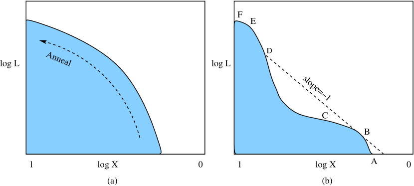
Another problem faced by thermodynamic integration is in navigating through phase changes as pointed out by Skilling (2004). As increases from 0 to 1, one hopes that the thermodynamic integration tracks gradually up in so inwards in as illustrated in Fig. 1(a). is related to the slope of curve as . This requires the log-likelihood curve to be concave as in Fig. 1(a). If the log-likelihood curve is non-concave as in Fig. 1(b), then increasing from 0 to 1 will normally take the samples from A to the neighbourhood of B where the slope is . In order to get the samples beyond B, will need to be taken beyond 1. Doing this will take the samples around the neighbourhood of the point of inflection C but here thermodynamic integration sees a phase change and has to jump across, somewhere near F, in which any practical computation exhibits hysteresis that destroys the calculation of . As will be discussed in the next section, nested sampling does not experience any problem with phase changes and moves steadily down in the prior volume regardless of whether the log-likelihood is concave or convex or even differentiable at all.
3 Nested sampling
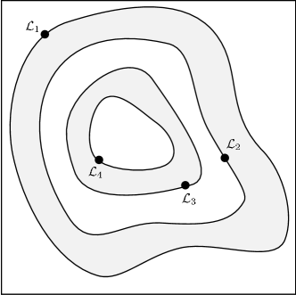
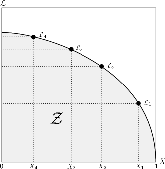
Nested sampling (Skilling 2004) is a Monte Carlo technique aimed at efficient evaluation of the Bayesian evidence, but also produces posterior inferences as a by-product. It exploits the relation between the likelihood and prior volume to transform the multidimensional evidence integral (2) into a one-dimensional integral. The ‘prior volume’ is defined by , so that
| (4) |
where the integral extends over the region(s) of parameter space contained within the iso-likelihood contour . Assuming that , i.e. the inverse of (4), is a monotonically decreasing function of (which is trivially satisfied for most posteriors), the evidence integral (2) can then be written as
| (5) |
Thus, if one can evaluate the likelihoods , where is a sequence of decreasing values,
| (6) |
as shown schematically in Fig. 2, the evidence can be approximated numerically using standard quadrature methods as a weighted sum
| (7) |
In the following we will use the simple trapezium rule, for which the weights are given by . An example of a posterior in two dimensions and its associated function is shown in Fig. 2.
3.1 Evidence evaluation
The nested sampling algorithm performs the summation (7) as follows. To begin, the iteration counter is set to and ‘live’ (or ‘active’) samples are drawn from the full prior (which is often simply the uniform distribution over the prior range), so the initial prior volume is . The samples are then sorted in order of their likelihood and the smallest (with likelihood ) is removed from the live set and replaced by a point drawn from the prior subject to the constraint that the point has a likelihood . The corresponding prior volume contained within this iso-likelihood contour will be a random variable given by , where follows the distribution (i.e. the probability distribution for the largest of samples drawn uniformly from the interval ). At each subsequent iteration , the discarding of the lowest likelihood point in the live set, the drawing of a replacement with and the reduction of the corresponding prior volume are repeated, until the entire prior volume has been traversed. The algorithm thus travels through nested shells of likelihood as the prior volume is reduced.
The mean and standard deviation of , which dominates the geometrical exploration, are:
| (8) |
Since each value of is independent, after iterations the prior volume will shrink down such that . Thus, one takes .
3.2 Stopping criterion
The nested sampling algorithm should be terminated on determining the evidence to some specified precision. One way would be to proceed until the evidence estimated at each replacement changes by less than a specified tolerance. This could, however, underestimate the evidence in (for example) cases where the posterior contains any narrow peaks close to its maximum. Skilling (2004) provides an adequate and robust condition by determining an upper limit on the evidence that can be determined from the remaining set of current active points. By selecting the maximum-likelihood in the set of active points, one can safely assume that the largest evidence contribution that can be made by the remaining portion of the posterior is , i.e. the product of the remaining prior volume and maximum likelihood value. We choose to stop when this quantity would no longer change the final evidence estimate by some user-defined value (we use 0.1 in log-evidence).
3.3 Posterior inferences
Once the evidence is found, posterior inferences can be easily generated using the full sequence of discarded points from the nested sampling process, i.e. the points with the lowest likelihood value at each iteration of the algorithm. Each such point is simply assigned the weight
| (9) |
These samples can then be used to calculate inferences of posterior parameters such as means, standard deviations, covariances and so on, or to construct marginalised posterior distributions.
3.4 Evidence error estimation
If we could assign each value exactly then the only error in our estimate of the evidence would be due to the discretisation of the integral (7). Since each is a random variable, however, the dominant source of uncertainty in the final value arises from the incorrect assignment of each prior volume. Fortunately, this uncertainty can be easily estimated.
Shaw et al. made use of the knowledge of the distribution from which each is drawn to assess the errors in any quantities calculated. Given the probability of the vector as
| (10) |
one can write the expectation value of any quantity as
| (11) |
Evaluation of this integral is possible by Monte Carlo methods by sampling a given number of vectors t and finding the average . By this method one can determine the variance of the curve in space, and thus the uncertainty in the evidence integral . As demonstrated by Shaw et al., this eliminates the need for any repetition of the algorithm to determine the standard error on the evidence value; this constitutes a significant increase in efficiency.
In our new methods presented below, however, we use a different error estimation scheme suggested by Skilling (2004); this also provides an error estimate in a single sampling but is far less computationally expensive and proceeds as follows. The usual behaviour of the evidence increments is initially to rise with iteration number , with the likelihood increasing faster than the weight decreases. At some point flattens off sufficiently that the decrease in the weight dominates the increase in likelihood, so the increment reaches a maximum and then starts to drop with iteration number. Most of the contribution to the final evidence value usually comes from the iterations around the maximum point, which occurs in the region of , where is the negative relative entropy,
| (12) |
where denotes the posterior. Since , we expect the procedure to take about steps to shrink down to the bulk of the posterior. The dominant uncertainty in is due to the Poisson variability in the number of steps to reach the posterior bulk. Correspondingly the accumulated values are subject to a standard deviation uncertainty of . This uncertainty is transmitted to the evidence through (7), so that also has standard deviation uncertainty of . Thus, putting the results together gives
| (13) |
Alongside the above uncertainty, there is also the error due to the discretisation of the integral in (7). Using the trapezoidal rule, this error will be , and hence will be negligible given a sufficient number of iterations.
4 Ellipsoidal nested sampling
The most challenging task in implementing the nested sampling algorithm is drawing samples from the prior within the hard constraint at each iteration . Employing a naive approach that draws blindly from the prior would result in a steady decrease in the acceptance rate of new samples with decreasing prior volume (and increasing likelihood).
4.1 Single ellipsoid sampling
Ellipsoidal sampling (Mukherjee et al. (2006)) partially overcomes the above problem by approximating the iso-likelihood contour of the point to be replaced by an -dimensional ellipsoid determined from the covariance matrix of the current set of live points. This ellipsoid is then enlarged by some factor to account for the iso-likelihood contour not being exactly ellipsoidal. New points are then selected from the prior within this (enlarged) ellipsoidal bound until one is obtained that has a likelihood exceeding that of the discarded lowest-likelihood point. In the limit that the ellipsoid coincides with the true iso-likelihood contour, the acceptance rate tends to unity. An elegant method for drawing uniform samples from an -dimensional ellipsoid is given by Shaw et al. (2007). and is easily extended to non-uniform priors.
4.2 Recursive clustering
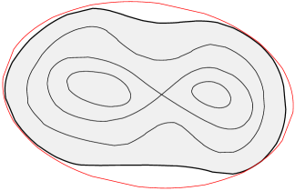
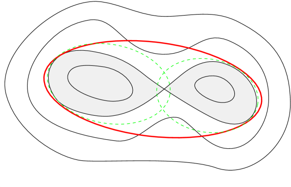
Ellipsoidal nested sampling as described above is efficient for simple unimodal posterior distributions, but is not well suited to multimodal distributions. The problem is illustrated in Fig. 3, in which one sees that the sampling efficiency from a single ellipsoid drops rapidly as the posterior value increases (particularly in higher dimensions). As advocated by Shaw et al., and illustrated in the final panel of the figure, the efficiency can be substantially improved by identifying distinct clusters of live points that are well separated and constructing an individual ellipsoid for each cluster. The linear nature of the evidence means it is valid to consider each cluster individually and sum the contributions provided one correctly assigns the prior volumes to each distinct region. Since the collection of active points is distributed evenly across the prior one can safely assume that the number of points within each clustered region is proportional to the prior volume contained therein.
Shaw et al. (2007) identify clusters recursively. Initially, at each iteration of the nested sampling algorithm, -means clustering (see e.g. MacKay (2003)) with is applied to the live set of points to partition them into two clusters and an (enlarged) ellipsoid is constructed for each one. This division of the live set will only be accepted if two further conditions are met: (i) the total volume of the two ellipsoids is less than some fraction of the original pre-clustering ellipsoid and (ii) clusters are sufficiently separated by some distance to avoid overlapping regions. If these conditions are satisfied clustering will occur and the number of live points in each cluster are topped-up to by sampling from the prior inside the corresponding ellipsoid, subject to the hard constraint . The algorithm then searches independently within each cluster attempting to divide it further. This process continues recursively until the stopping criterion is met. Shaw et al. also show how the error estimation procedure can be modified to accommodate clustering by finding the probability distribution of the volume fraction in each cluster.
5 Improved ellipsoidal sampling methods
In this section, we present two new methods for ellipsoidal nested sampling that improve significantly in terms of sampling efficiency and robustness on the existing techniques outlined above, in particular for multimodal distributions and those with pronounced degeneracies.
5.1 General improvements
We begin by noting several general improvements that are employed by one or other of our new methods.
5.1.1 Identification of clusters
In both methods, we wish to identify isolated modes of the posterior distribution without prior knowledge of their number. The only information we have is the current live point set. Rather than using -means clustering with to partition the points into just two clusters at each iteration, we instead attempt to infer the appropriate number of clusters from the point set. After experimenting with several clustering algorithms to partition the points into the optimal number of clusters, we found X-means (Pelleg et al., 2000), G-means (Hamerly et al., 2003) and PG-means (Feng et al., 2006) to be the most promising. X-means partitions the points into the number of clusters that optimizes the Bayesian Information Criteria (BIC) measure. The G-means algorithm is based on a statistical test for the hypothesis that a subset of data follows a Gaussian distribution and runs -means with increasing in a hierarchical fashion until the test accepts the hypothesis that the data assigned to each -means centre are Gaussian. PG-means is an extension of G-means that is able to learn the number of clusters in the classical Gaussian mixture model without using -means. We found PG-means to outperform both X-means and G-means, especially in higher dimensions and if there are cluster intersections, but the method requires Monte Carlo simulations at each iteration to calculate the critical values of the Kolmogorov–Smirnov test it uses to check for Gaussianity. As a result, PG-means is considerably more computationally expensive than both X-means and G-means, and this computational cost quickly becomes prohibitive. Comparing X-means and G-means, we found the former to produce more consistent results, particularly in higher dimensions. Since we have to cluster the live points at each iteration of the nested sampling process, we thus chose to use the X-means clustering algorithm. This method performs well overall, but does suffers from some occasional problems that can result in the number of clusters identified being more or less than the actual number. We discuss these problems in the context of both our implementations in sections 5.2 and 5.3 but conclude they do not adversely affect out methods. Ideally, we require a fast and robust clustering algorithm that always produces reliable results, particularly in high dimensions. If such a method became available, it could easily be substituted for X-means in either of our sampling techniques described below.
5.1.2 Dynamic enlargement factor
Once an ellipsoid has been constructed for each identified cluster such that it (just) encloses all the corresponding live points, it is enlarged by some factor , as discussed in Sec. 4. It is worth remembering that the corresponding increase in volume is , where is the dimension of the parameter space. The factor does not, however, have to remain constant. Indeed, as the nested sampling algorithm moves into higher likelihood regions (with decreasing prior volume), the enlargement factor by which an ellipsoid is expanded can be made progressively smaller. This holds since the ellipsoidal approximation to the iso-likelihood contour obtained from the live points becomes increasingly accurate with decreasing prior volume.
Also, when more than one ellipsoid is constructed at some iteration, the ellipsoids with fewer points require a higher enlargement factor than those with a larger number of points. This is due to the error introduced in the evaluation of the eigenvalues from the covariance matrix calculated from a limited sample size. The standard deviation uncertainty in the eigenvalues is given by Girshick (1939) as follows:
| (14) |
where denotes the th eigenvalue and is the number of points used in the calculation of the covariance matrix.
The above considerations lead us to set the enlargement factor for the th ellipsoid at iteration as where is the total number of live points, is the initial user–defined enlargement factor (defining the percentage by which each axis of an ellipsoid enclosing points, is enlarged), is the prior volume at the th iteration, is the number of points in the cluster, and is a value between and that defines the rate at which the enlargement factor decreases with decreasing prior volume.
5.1.3 Detection of overlapping ellipsoids
In some parts of our sampling methods, it is important to have a very fast method to determine whether two ellipsoids intersect, as this operation is performed many times at each iteration. Rather than applying the heuristic criteria used by Shaw et al., we instead employ an exact algorithm proposed by Alfano et al. (2003) which involves the calculation of eigenvalues and eigenvectors of the covariance matrix of the points in each ellipsoid. Since we have already calculated these quantities in constructing the ellipsoids, we can rapidly determine if two ellipsoids intersect at very little extra computational cost.
5.1.4 Sampling from overlapping ellipsoids
As illustrated earlier in Fig. 3, for a multimodal distribution multiple ellipsoids represent a much better approximation to the iso-likelihood contour than a single ellipsoid containing all the live points. At likelihood levels around which modes separate, X-means will often partition the point set into a number of distinct clusters, but the (enlarged) ellipsoids enclosing distinct identified clusters will tend to overlap (see Fig. 4) and the partitioning will be discarded. At some sufficiently higher likelihood level, the corresponding ellipsoids will usually no longer overlap, but it is wasteful to wait for this to occur. Hence, in both of our new sampling methods described below it will prove extremely useful to be able to sample consistently from ellipsoids that may be overlapping, without biassing the resultant evidence value or posterior inferences.
Suppose at iteration of the nested sampling algorithm, a set of live points is partitioned into clusters by X-means, with the cluster having points. Using the covariance matrices of each set of points, each cluster then is enclosed in an ellipsoid which is then expanded using an enlargement factor . The volume of each resulting ellipsoid is then found and one ellipsoid is chosen with probability equal to its volume fraction:
| (15) |
where . Samples are then drawn from the chosen ellipsoid until a sample is found for which the hard constraint is satisfied, where is the lowest-likelihood value among all the live points under consideration. There is, of course, a possibility that the chosen ellipsoid overlaps with one or more other ellipsoids. In order to take an account of this possibility, we find the number of ellipsoids, , in which the sample lies and only accept the sample with probability . This provides a consistent sampling procedure in all cases.
5.2 Method 1: simultaneous ellipsoidal sampling
This method is built in large part around the above technique for sampling consistently from potentially overlapping ellipsoids. At each iteration of the nested sampling algorithm, the method proceeds as follows. The full set of live points is partitioned using X-means, which returns clusters with points respectively. For each cluster, the covariance matrix of the points is calculated and used to construct an ellipsoid that just encloses all the points; each ellipsoid is then expanded by the enlargement factor (which can depend on iteration number as well as the number of points in the th ellipsoid, as outlined above). This results in a set of ellipsoids at each iteration, which we refer to as sibling ellipsoids. The lowest-likelihood point (with likelihood ) from the full set of live points is then discarded and replaced by a new point drawn from the set of sibling ellipsoids, correctly taking into account any overlaps.
It is worth noting that at early iterations of the nested sampling process, X-means usually identifies only cluster and the corresponding (enlarged) ellipsoid completely encloses the prior range, in which case sampling is performed from the prior range instead. Beyond this minor inconvenience, it is important to recognise that any drawbacks of the X-means clustering method have little impact on the accuracy of the calculated evidence or posterior inferences. We use X-means only to limit the remaining prior space from which to sample, in order to increase efficiency. If X-means returns greater or fewer than the desired number of clusters, one would still sample uniformly from the remaining prior space since the union of the corresponding (enlarged) ellipsoids would still enclose all the remaining prior volume. Hence, the evidence calculated and posterior inferences would remain accurate to within the uncertainties discussed in Sec. 3.4.
5.3 Method 2: clustered ellipsoidal sampling
This method is closer in spirit to the recursive clustering technique advocated by Shaw et al. At the th iteration of the nested sampling algorithm, the method proceeds as follows. The full set of live points is again partitioned using X-means to obtain clusters with points respectively, and each cluster is enclosed in an expanded ellipsoid as outlined above. In this second approach, however, each ellipsoid is then tested to determine if it intersects with any of its sibling ellipsoids or any other non-ancestor ellipsoid111A non-ancestor ellipsoid of is any ellipsoid that was non-intersecting at an earlier iteration and does not completely enclose .. The nested sampling algorithm is then continued separately for each cluster contained within a non-intersecting ellipsoid , after in each case (i) topping up the number of points to by sampling points within that satisfy ; and (ii) setting the corresponding remaining prior volume to . Finally, the remaining set of points contained within the union of the intersecting ellipsoids at iteration is topped up to using the method for sampling from such a set of ellipsoids outlined in Sec. 5.1.4, and the associated remaining prior volume is set to .
As expected, in the early stages, X-means again usually identifies only cluster and this is dealt with as in Method 1. Once again, the drawbacks of X-means do not have much impact on the accuracy of the global evidence determination. If X-means finds fewer clusters than the true number of modes, then some clusters correspond to more than one mode and will have an enclosing ellipsoid larger than it would if X-means had done a perfect job; this increases the chances of the ellipsoid intersecting with some of its sibling or non-ancestor ellipsoids. If this ellipsoid is non-intersecting, then it can still split later and hence we do not lose accuracy. On the other hand, if X-means finds more clusters than the true number of modes, it is again likely that the corresponding enclosing ellipsoids will overlap. It is only in the rare case where some of such ellipsoids are non-intersecting, that the possibility exists for missing part of the true prior volume. Our use of an enlargement factor strongly mitigates against this occurring. Indeed, we have not observed such behaviour in any of our numerical tests.
5.4 Evaluating ‘local’ evidences
For a multimodal posterior, it can prove useful to estimate not only the total (global) evidence, but also the ‘local’ evidences associated with each mode of the distribution. There is inevitably some arbitrariness in defining these quantities, since modes of the posterior necessarily sit on top of some general ‘background’ in the probability distribution. Moreover, modes lying close to one another in the parameter space may only ‘separate out’ at relatively high likelihood levels. Nonetheless, for well-defined, isolated modes, a reasonable estimate of the posterior volume that each contains (and hence the local evidence) can be defined and estimated. Once the nested sampling algorithm has progressed to a likelihood level such that (at least locally) the ‘footprint’ of the mode is well-defined, one needs to identify at each subsequent iteration those points in the live set belonging to that mode. The practical means of performing this identification and evaluating the local evidence for each mode differs between our two sampling methods.
5.4.1 Method 1
The key feature of this method is that at each iteration the full live set of points is evolved by replacing the lowest likelihood point with one drawn (consistently) from the complete set of (potentially overlapping) ellipsoids. Thus, once a likelihood level is reached such that the footprint of some mode is well defined, to evaluate its local evidence one requires that at each subsequent iteration the points associated with the mode are consistently identified as a single cluster. If such an identification were possible, at the th iteration one would simply proceeds as follows: (i) identify the cluster (contained within the ellipsoid ) to which the point with the lowest likelihood value belongs; (ii) update the local prior volume of each of the clusters as , where is the number of points belonging to the th cluster and is the total remaining prior volume; (iii) increment the local evidence of the cluster contained within by . Unfortunately, we have found that X-means is not capable of consistently identifying the points associated with some mode as a single cluster. Rather, the partitioning of the live point set into clusters can vary appreciably from one iteration to the next. PG-means produced reasonably consistent results, but as mentioned above is far too computationally intensive. We are currently exploring ways to reduce the most computationally expensive step in PG-means of calculating the critical values for Kolmogorov–Smirnov test, but this is not yet completed. Thus, in the absence of a fast and consistent clustering algorithm, it is currently not possible to calculate the local evidence of each mode with our simultaneous ellipsoidal sampling algorithm.
5.4.2 Method 2
The key feature of this method is that once a cluster of points has been identified such that its (enlarged) enclosing ellipsoid does not intersect with any of its sibling ellipsoids (or any other non-ancestor ellipsoid), that set of points is evolved independently of the rest (after topping up the number of points in the cluster to ). This approach therefore has some natural advantages in evaluating local evidences. There remain, however, some problems associated with modes that are sufficiently close to one another in the parameter space that they are only identified as separate clusters (with non-intersecting enclosing ellipsoids) once the algorithm has proceeded to likelihood values somewhat larger than the value at which the modes actually separate. In such cases, the local evidence of each mode will be underestimated. The simplest solution to this problem would be to increment the local evidence of each cluster even if its corresponding ellipsoid intersects with other ellipsoids, but as mentioned above X-means cannot produce the consistent clustering required. In this case we have the advantage of knowing the iteration beyond which a non-intersecting ellipsoid is regarded as a separate mode (or a collection of modes) and hence we can circumvent this problem by storing information (eigenvalues, eigenvectors, enlargement factors etc.) of all the clusters identified, as well as the rejected points and their likelihood values, from the last few iterations. We then attempt to match the clusters in the current iteration to those identified in the last few iterations, allowing for the insertion or rejection of points from clusters during the intervening iterations On finding a match for some cluster in a previous iteration , we check to see which (if any) of the points discarded between the iteration and the current iteration were members of the cluster. For each iteration (between and inclusive) where this occurs, the local evidence of the cluster is incremented by , where and are the lowest likelihood value and the remaining prior volume corresponding to iteration . This series of operations can be performed quite efficiently; even storing information as far as back as 15 iterations does not increase the running time of the algorithm appreciably. Finally, we note that if closely lying modes have very different amplitudes, the mode(s) with low amplitude may never be identified as being separate and will eventually be lost as the algorithm moves to higher likelihood values.
5.5 Dealing with degeneracies
As will be demonstrated in Sec. 7, the above methods are very efficient and robust at sampling from multimodal distributions where each mode is well-described at most likelihood levels by a multivariate Gaussian. Such posteriors might be described colloquially as resembling a ‘bunch of grapes’ (albeit in many dimensions). In some problems, however, some modes of the posterior might possess a pronounced curving degeneracy so that it more closely resembles a (multidimensional) ‘banana’. Such features are problematic for all sampling methods, including our proposed ellipsoidal sampling techniques. Fortunately, we have found that a simple modification to our methods allows for efficient sampling even in the presence of pronounced degeneracies.
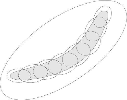
The essence of the modification is illustrated in Fig. 5. Consider an isolated mode with an iso-likelihood contour displaying a pronounced curved degeneracy. X-means will usually identify all the live points contained within it as belonging to a single cluster and hence the corresponding (enlarged) ellipsoid will represent a very poor approximation. If, however, one divides each cluster identified by X-means into a set of sub-clusters, one can more accurately approximate the iso-likelihood contour with many small overlapping ellipsoids and sample from them using the method outlined in Sec. 5.1.4.
To sample with maximum efficiency from a pronounced degeneracy (particularly in higher dimensions), one would like to divide every cluster found by X-means into as many sub-clusters as possible to allow maximum flexibility in following the degeneracy. In order to be able to calculate covariance matrices, however, each sub-cluster must contain at least points, where is the dimensionality of the parameter space. This in turn sets an upper limit on the number of sub-clusters.
Sub-clustering is performed through an incremental -means algorithm with . The process starts with all the points assigned to the original cluster. At iteration of the algorithm, a point is picked at random from the sub-cluster that contains the most points. This point is then set as the centroid, , of a new cluster . All those points in any of the other sub-clusters that are closer to than the centroid of their own sub-cluster, and whose sub-cluster has more than points are then assigned to and is updated. All the points not belonging to are again checked with the updated until no new point is assigned to . At the end of the iteration , if has less than points then the points in that are closest to are assigned to until has points. In the case that has fewer than points, then points are assigned from to . The algorithm stops when, at the start of an iteration, the sub-cluster with most points has fewer than members, since that would result in a new sub-cluster with fewer than points. This process can result in quite a few sub-clusters with more than but less than points and hence there is a possibility for even more sub-clusters to be formed. This is achieved by finding the sub-cluster closest to the cluster, . If the sum of points in and is greater than or equal to , an additional sub-cluster is created out of them.
Finally, we further reduce the possibility that the union of the ellipsoids corresponding to different sub-clusters might not enclose the entire remaining prior volume as follows. For each sub-cluster , we find the one point in each of the nearest sub-clusters that is closest to the centroid of . Each such point is then assigned to and its original sub-cluster, i.e. it is ‘shared’ between the two sub-clusters. In this way all the sub-clusters and their corresponding ellipsoids are expanded, jointly enclosing the whole of the remaining prior volume. In our numerical simulations, we found setting performs well.
6 Metropolis Nested Sampling
An alternative method for drawing samples from the prior within the hard constraint where is the lowest likelihood value at iteration , is the standard Metropolis algorithm (see e.g. MacKay (2003)) as suggested in Sivia et al. (2006). In this approach, at each iteration, one of the live points, , is picked at random and a new trial point, , is generated using a symmetric proposal distribution . The trial point is then accepted with probability
| (16) |
A symmetric Gaussian distribution is often used as the proposal distribution. The dispersion of this Gaussian should be sufficiently large compared to the size of the region satisfying that the chain is reasonably mobile, but without being so large that the likelihood constraint stops nearly all proposed moves. Since an independent sample is required, steps are taken by the Metropolis algorithm so that the chain diffuses far away from the starting position and the memory of it is lost. In principle, one could calculate convergence statistics to determine at which point the chain is sampling from the target distribution. Sivia et al. (2006) propose, however, that one should instead simply take steps in all cases. The appropriate value of tends to diminish as the nested algorithm moves towards higher likelihood regions and decreasing prior mass. Hence, the value of is updated at the end of each nested sampling iteration, so that the acceptance rate is around 50%, as follows:
| (17) |
where and are the numbers of accepted and rejected samples in the latest Metropolis sampling phase.
In principle, this approach can be used quite generally and does not require any clustering of the live points or construction of ellipsoidal bounds. In order to facilitate the evaluation of ‘local’ evidences, however, we combine this approach with the clustering process performed in Method 2 above to produce a hybrid algorithm, which we describe below. Moreover, as we show in Section 7.1, this hybrid approach is significantly more efficient in sampling from multimodal posteriors than using just the Metropolis algorithm without clustering.
At each iteration of the nested sampling process, the set of live points is partitioned into clusters, (enlarged) enclosing ellipsoids are constructed, and overlap detection is performed precisely in the clustered ellipsoidal method. Once again, the nested sampling algorithm is then continued separately for each cluster contained within a non-intersecting ellipsoid . This proceeds by (i) topping up the number of points in each cluster to by sampling points that satisfy using the Metropolis method described above, and (ii) setting the corresponding remaining prior mass to . Prior to topping up a cluster in step (i), a ‘mini’ burn-in is performed during which the width of the proposal distribution is adjusted as described above; the width is then kept constant during the topping-up step.
During the sampling the starting point for the random walk is chosen by picking one of the ellipsoids with probability equal to its volume fraction:
| (18) |
where is the volume occupied by the ellipsoid and , and then picking randomly from the points lying inside the chosen ellipsoid. This is done so that the number of points inside the modes is proportional to the prior volume occupied by those modes. We also supplement the condition (16) for a trial point to be accepted by the requirement that it must not lie inside any of the non-ancestor ellipsoids in order to avoid over-sampling any region of the prior space. Moreover, in step (i) if any sample accepted during the topping-up step lies outside its corresponding (expanded) ellipsoid, then that ellipsoid is dropped from the list of those to be explored as an isolated likelihood region in the current iteration since that would mean that the region has not truly separated from the rest of the prior space.
Metropolis nested sampling can be quite efficient in higher-dimensional problems as compared with the ellipsoidal sampling methods since, in such cases, even a small region of an ellipsoid lying outide the true iso-likelihood contour would occupy a large volume and hence result in a large drop in efficiency. Metropolis nested sampling method does not suffer from this curse of dimensionality as it only uses the ellipsoids to separate the isolated likelihood regions and consequently the efficiency remains approximately constant at , which is per cent in our case. This will be illustrated in the next section in which Metropolis nested sampling is denoted as Method 3.
7 Applications
In this section we apply the three new algorithms discussed in the previous sections to two toy problems to demonstrate that they indeed calculate the Bayesian evidence and make posterior inferences accurately and efficiently.
7.1 Toy model 1
For our first example, we consider the problem investigated by Shaw et al. (2007) as their Toy Model II, which has a posterior of known functional form so that an analytical evidence is available to compare with those found by our nested sampling algorithms. The two-dimensional posterior consists of the sum of 5 Gaussian peaks of varying width, , and amplitude, , placed randomly within the unit circle in the -plane. The parameter values defining the Gaussians are listed in Table 1, leading to an analytical total log-evidence . The analytical ‘local’ log-evidence associated with each of the 5 Gaussian peaks is also shown in the table.
| Peak | Local | ||||
|---|---|---|---|---|---|
| 1 | |||||
| 2 | |||||
| 3 | |||||
| 4 | |||||
| 5 |
| Toy model 1a | Method 1 | Method 2 | Method 3 | Shaw et al. |
|---|---|---|---|---|
| Error | 0.110 | 0.112 | 0.115 | 0.084 |
| 39,911 | 12,569 | 161,202 | 101,699 |
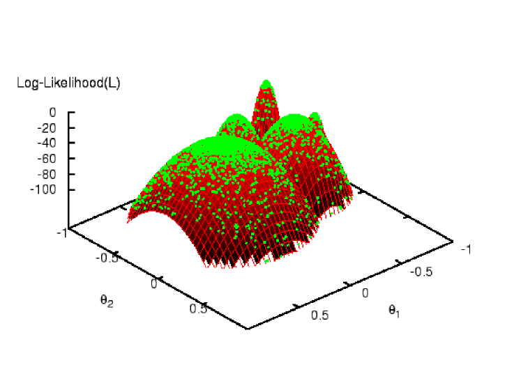
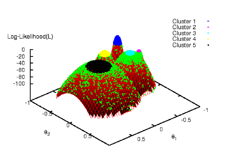
The results of applying Method 1 (simultaneous ellipsoidal sampling), Method 2 (clustered ellipsoidal sampling) to this problem are illustrated in Figs 6 and 7 respectively; a very similar plot to Fig. 7 is obtained for Method 3 (Metropolis nested sampling). For all three methods, we used live points, switched off the sub-clustering modification (for methods 1 and 2) outlined in Sec. 5.5, and assumed a flat prior within the unit circle for the parameters and in this two-dimensional problem. In each figure, the dots denote the set of live points at each successive likelihood level in the nested sampling algorithm. For methods 2 and 3, the different colours denote points assigned to isolated clusters as the algorithm progresses. We see that all three algorithms sample effectively from all the peaks, even correctly isolating the narrow Gaussian peak (cluster 2) superposed on the broad Gaussian mode (cluster 3).
The global log-evidence values, their uncertainties and the number of likelihood evaluations required for each method are shown in Table 2. Methods 1, 2 and 3, all produce evidence values that are accurate to within the estimated uncertainties. Also, listed in the table are the corresponding quantities obtained by Shaw et al. (2007), which are clearly consistent. Of particular interest, is the number of likelihood evaluations required to produce these evidence estimates. Methods 1 and 2 made around 40,000 and 10,000 likelihood evaluations respectively, whereas the Shaw et al. method required more than 3 times this number (in all cases just one run of the algorithm was performed, since multiple runs are not required to estimate the uncertainty in the evidence). Method 3 required about 170,000 likelihood evaluations since its efficiency remains constant at around 5%. It should be remembered that Shaw et al. showed that using thermodynamic integration, and performing 10 separate runs to estimate the error in the evidence, required likelihood evaluations to reach the same accuracy. As an aside, we also investigated a ‘vanilla’ version of the Metropolis nested sampling approach, in which no clustering was performed. In this case, over 570,000 likelihood evaluations were required to estimate the evidence to the same accuracy. This drop in efficieny relative to Method 3 resulted from having to sample inside different modes using a proposal distribution with the same width in every case. This leads to a high rejection rate inside narrow modes and random walk behaviour in the wider modes. In higher dimensions this effect will be exacerbated. Consequently, the clustering process seems crucial for sampling efficiently from multimodal distributions of different sizes using Metropolis nested sampling.
Using methods 2 (clustered ellipsoidal sampling) and 3 (Metropolis sampling) it is possible to calculate the ‘local’ evidence and make posterior inferences for each peak separately. For Method 2, the mean values inferred for the parameters and and the local evidences thus obtained are listed in Table 3, and clearly compare well with the true values given in Table 1. Similar results were obtained using Method 3.
| Peak | Local | ||
|---|---|---|---|
| 1 | |||
| 2 | |||
| 3 | |||
| 4 | |||
| 5 |
In real applications the parameter space is usually of higher dimension and different modes of the posterior may vary in amplitude by more than an order of magnitude. To investigate this situation, we also considered a modified problem in which three 10-dimensional Gaussians are placed randomly in the unit hypercube and have amplitudes differing by two orders of magnitude. We also make one of the Gaussians elongated. The analytical local log-evidence values and those found by applying Method 2 (without sub-clustering) and Method 3 are shown in Table 4. We used live points with both of our methods.
| Toy model 1b | Real Value | Method 2 | Method 3 |
|---|---|---|---|
| 4.66 | 4.470.20 | 4.520.20 | |
| local | 4.61 | 4.380.20 | 4.400.21 |
| local | 1.78 | 1.990.21 | 2.150.21 |
| local | 0.00 | 0.090.20 | 0.090.20 |
| 130,529 | 699,778 |
We see that both methods detected all 3 Gaussians and calculated their evidence values with reasonable accuracy within the estimated uncertainties. Method 2 required times fewer likelihood calculations than Method 3, since in this problem the ellipsoidal methods can still achieve very high efficiency (28 per cent), while the efficiency of the Metropolis method remains constant (5 per cent) as discussed in Sec. 6.
7.2 Toy model 2
We now illustrate the capabilities of our methods in sampling from a posterior containing multiple modes with pronounced (curving) degeneracies in high dimensions. Our toy problem is based on that investigated by Allanach et al. (2007), but we extend it to more than two dimensions.
The likelihood function is defined as,
| (19) |
where
| (20) |
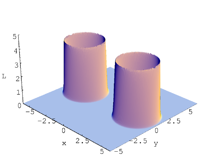
In 2-dimensions, this toy distribution represents two well separated rings, centred on the points and respectively, each of radius and with a Gaussian radial profile of width (see Fig. 8). With a sufficiently small value, this distribution is representative of the likelihood functions one might encounter in analysing forthcoming particle physics experiments in the context of beyond-the-Standard-Model paradigms; in such models the bulk of the probability lies within thin sheets or hypersurfaces through the full parameter space.
We investigate the above distribution up to a -dimensional parameter space . In all cases, the centers of the two rings are separated by units in the parameter space, and we take and . We make and equal, since in higher dimensions any slight difference between these two would result in a vast difference between the volumes occupied by the rings and consequently the ring with the smaller value would occupy vanishingly small probability volume making its detection almost impossible. It should also be noted that setting means the rings have an extremely narrow Gaussian profile and hence they represent an ‘optimally difficult’ problem for our ellipsoidal nested sampling algorithms, even with sub-clustering, since many tiny ellipsoids are required to obtain a sufficiently accurate representation of the iso-likelihood surfaces. For the two-dimensional case, with the parameters described above, the likelihood function is that shown in Fig. 8.
Sampling from such a highly non-Gaussian and curved distribution can be very difficult and inefficient, especially in higher dimensions. In such problems a re-parameterization is usually performed to transform the distribution into one that is geometrically simpler (see e.g. Dunkley et al. (2005) and Verde et al. (2003)), but such approaches are generally only feasible in low-dimensional problems. In general, in dimensions, the transformations usually employed introduce additional curvature parameters and hence become rather inconvenient. Here, we choose not to attempt a re-parameterization, but instead sample directly from the distribution.
| Analytical | Method 2 (with sub-clustering) | Method 3 | ||||||
|---|---|---|---|---|---|---|---|---|
| local | local | local | local | local | ||||
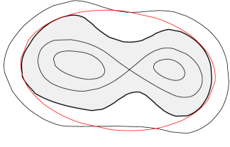
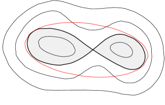
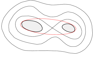
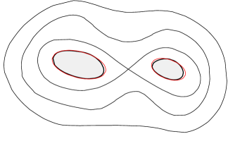
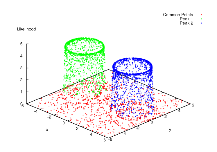
Applying the ellipsoidal nested sampling approaches (methods 1 and 2) to this problem without using the sub-clustering modification would result in highly inefficient sampling as the enclosing ellipsoid would represent an extremely poor approximation to the ring. Thus, for this problem, we use Method 2 with sub-clustering and Method 3 (Metropolis nested sampling). We use live points in both algorithms. The sampling statistics are listed in Table 5 and Table 6 respectively. The 2-dimensional sampling results using Method 2 (with sub-clustering) are also illustrated in Fig. 9, in which the set of live points at each successive likelihood level is plotted; similar results are obtained using Method 3.
We see that both methods produce reliable estimates of the global and local evidences as the dimension of the parameter space increases. As seen in Table 6, however, the efficieny of Method 2, even with sub-clustering, drops significantly with increasing dimensionality. As a result, we do not explore the problem with method 2 for dimensions greater than . This drop in efficiency is caused by (a) in higher dimensions even a small region of an ellipsoid that lies outside the true iso-likelihood contour occupies a large volume and hence results in a drop in sampling efficiency; and (b) in dimensions, the minimum number of points in an ellipsoid can be , as discussed in Sec. 5.5, and consequently with a given number of live points, the number of sub-clusters decreases with increasing dimensionality, resulting in a poor approximation to the highly curved iso-likelihood contour. Nonetheless, Method 3 is capable of obtaining evidence estimates with reasonable efficiency up to , and should continue to operate effectively at even higher dimensionality.
| Method 2 (with sub-clustering) | Method 3 | |||
|---|---|---|---|---|
| Efficiency | Efficiency | |||
8 Bayesian object detection
We now consider how our multimodal nested sampling approaches may be used to address the difficult problem of detecting and characterizing discrete objects hidden in some background noise. A Bayesian approach to this problem in an astrophysical context was first presented by Hobson & McLachlan (2003; hereinafter HM03), and our general framework follows this closely. For brevity, we will consider our data vector to denote the pixel values in a single image in which we wish to search for discrete objects, although could equally well represent the Fourier coefficients of the image, or coefficients in some other basis.
8.1 Discrete objects in background
Let us suppose we are interested in detecting and characterising some set of (two-dimensional) discrete objects, each of which is described by a template , which is parametrised in terms of a set of parameters that might typically denote (collectively) the position of the object, its amplitude and some measure of its spatial extent. In particular, in this example we will assume circularly-symmetric Gaussian-shaped objects defined by
| (21) |
so that . If such objects are present and the contribution of each object to the data is additive, we may write
| (22) |
where denotes the contribution to the data from the th discrete object and denotes the generalised ‘noise’ contribution to the data from other ‘background’ emission and instrumental noise. Clearly, we wish to use the data to place constraints on the values of the unknown parameters and .
8.2 Simulated data
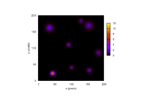
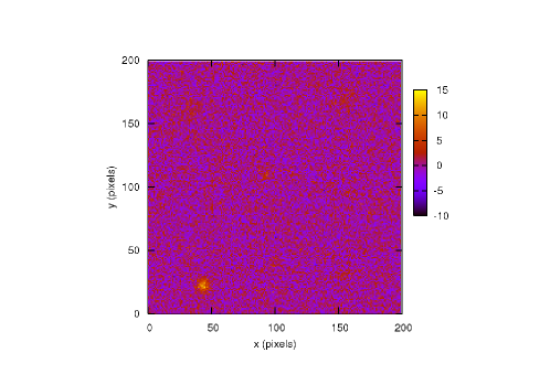
Our underlying model and simulated data are shown in Fig. 10, and are similar to the example considered by HM03. The left panel shows the pixel test image, which contains 8 Gaussian objects described by eq. (21) with the parameters , , and listed in Table 7. The and coordinates are drawn independently from the uniform distribution . Similarly, the amplitude and size of each object are drawn independently from the uniform distributions and respectively. We multiply the amplitude of the first object by to to see how senstive our nested sampling methods are to this order of magnitude difference in amplitudes. The simulated data map is created by adding independent Gaussian pixel noise with an rms of 2 units. This corresponds to a signal-to-noise ratio 0.5-1 as compared to the peak amplitude of each object (ignoring the first object). It can be seen from the figure that with this level of noise, apart from the first object, only a few objects are (barely) visible with the naked eye and there are certain areas where the noise conspires to give the impression of an object where none is present. This toy problem thus presents a considerable challenge for any object detection algorithm.
| Object | ||||
|---|---|---|---|---|
| 1 | 43.71 | 22.91 | 10.54 | 3.34 |
| 2 | 101.62 | 40.60 | 1.37 | 3.40 |
| 3 | 92.63 | 110.56 | 1.81 | 3.66 |
| 4 | 183.60 | 85.90 | 1.23 | 5.06 |
| 5 | 34.12 | 162.54 | 1.95 | 6.02 |
| 6 | 153.87 | 169.18 | 1.06 | 6.61 |
| 7 | 155.54 | 32.14 | 1.46 | 4.05 |
| 8 | 130.56 | 183.48 | 1.63 | 4.11 |
8.3 Defining the posterior distribution
As discussed in HM03, in analysing the above simulated data map the Bayesian purist would attempt to infer simultaneously the full set of parameters . The crucial complication inherent to this approach is that the length of the parameter vector is variable, since it depends on the unknown value . Thus any sampling based approach must be able to move between spaces of different dimensionality, and such techniques are investigated in HM03.
An alternative approach, also discussed by HM03, is simply to set . In other words, the model for the data consists of just a single object and so the full parameter space under consideration is , which is fixed and only 4-dimensional. Although fixing , it is important to understand that this does not restrict us to detecting just a single object in the data map. Indeed, by modelling the data in this way, we would expect the posterior distribution to possess numerous local maxima in the 4-dimensional parameter space, each corresponding to the location in this space of one of the objects present in the image. HM03 show this vastly simplified approach is indeed reliable when the objects of interest are spatially well-separated, and so for illustration we adopt this method here.
In this case, if the background ‘noise’ is a statistically homogeneous Gaussian random field with covariance matrix , then the likelihood function takes the form
| (23) |
In our simple problem the background is just independent pixel noise, so , where is the noise rms. The prior on the parameters is assumed to be separable, so that
| (24) |
The priors on and are taken to be the uniform distribution , whereas the priors on and are taken as the uniform distributions and respectively.
The problem of object identification and characterization then reduces to sampling from the (unnormalised) posterior to infer parameter values and calculating the ‘local’ Bayesian evidence for each detected object to assess the probability that it is indeed real. In the most straightforward approach, the two competing models between which we must select are ‘the detected object is fake ’ and ‘the detected object is real ’. One could, of course, consider alternative definitions of these hypotheses, such as setting : and : , where is some (non-zero) cut-off value below which one is not interested in the identified object.
8.4 Results
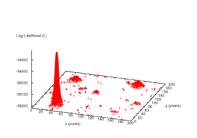
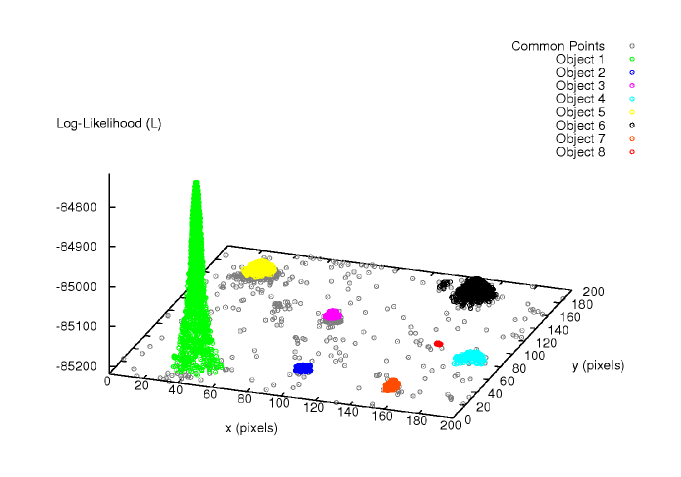
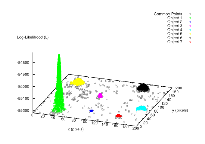
Since Bayesian object detection is of such interest, we analyse this problem using methods 1, 2 and 3. For methods 1 and 2, do not use sub-clustering, since the posterior peaks are not expected to exhibit pronounced (curving) degeneracies. We use 400 live points with method 1 and 300 with methods 2 and 3. In methods 1 and 2, the initial enlargement factor was set to .
In Fig. 11 we plot the live points, projected into the -subspace, at each successive likelihood level in the nested sampling algorithm (above an arbitrary base level) for each method. For the methods 2 and 3 results, plotted in panel (b) and (c) respectively, the different colours denote points assigned to isolated clusters as the algorithm progresses; we note that the base likelihood level used in the figure was chosen to lie slightly below that at which the individual clusters of points separate out. We see from the figure, that all three approaches have successfully sampled from this highly multimodal posterior distribution. As discussed in HM03, this represents a very difficult problem for traditional MCMC methods, and illustrates the clear advantages of our methods. In detail, the figure shows that samples are concentrated in 8 main areas. Comparison with Fig. 10 shows that 7 of these regions do indeed correspond to the locations of the real objects (one being a combination of two real objects), whereas the remaining cluster corresponds to a ‘conspiration’ of the background noise field. The CPU time required for Method 1 was only minutes on a single Itanium 2 (Madison) processor of the Cosmos supercomputer; each processor has a clock speed of 1.3 GHz, a 3Mb L3 cache and a peak performance of 5.2 Gflops.
| Method 1 | Method 2 | Method 3 | |
| (no sub-clustering) | (no sub-clustering) | ||
| Error | 0.20 | 0.24 | 0.24 |
| 55,521 | 74,668 | 478,557 |
| Cluster | local | ||||
|---|---|---|---|---|---|
| 1 | 43.82 0.05 | 23.17 0.05 | 10.33 0.15 | 3.36 0.03 | |
| 2 | 100.10 0.26 | 40.55 0.32 | 1.93 0.16 | 2.88 0.15 | |
| 3 | 92.82 0.14 | 110.17 0.16 | 3.77 0.26 | 2.42 0.13 | |
| 4 | 182.33 0.48 | 85.85 0.43 | 1.11 0.07 | 4.85 0.30 | |
| 5 | 33.96 0.36 | 161.50 0.35 | 1.56 0.09 | 6.28 0.29 | |
| 6 | 155.21 0.31 | 169.76 0.32 | 1.69 0.09 | 6.48 0.24 | |
| 7 | 154.87 0.32 | 31.59 0.22 | 1.98 0.17 | 3.16 0.20 | |
| 8 | 158.12 0.17 | 96.17 0.19 | 2.02 0.10 | 2.15 0.09 |
The global evidence results are summarised in Table 8. We see that all three approaches yield consistent values within the estimated uncertainties, which is very encouraging given their considerable algorithmic differences.
We note, in particular, that Method 3 required more than 6 times the number of likelihood evaluations as compared to the ellipsoidal methods. This is to be expected given the non-degenerate shape of the posterior modes and the low-dimensionality of this problem. The global evidence value of may be interpreted as corresponding to the model ‘there is a real object somewhere in the image’. Comparing this with the ‘null’ evidence value for ‘there is no real object in the image’, we see that is strongly favoured, with a log-evidence difference of .
In object detection, however, one is more interested in whether or not to believe the individual objects identified. As discussed in Sections 5.3 and 5.4, using Method 2 and Method 3, samples belonging to each identified mode can be separated and local evidences and posterior inferences calculated. In Table 9, for each separate cluster of points, we list the mean and standard error of the inferred object parameters and the local -evidence obtained using method 2; similar results are obtained from Method 3. Considering first the local evidences and comparing them with the ‘null’ evidence of , we see that all the identified clusters should be considered as real detections, except for cluster 8. Comparing the derived object parameters with the inputs listed in Table 7, we see that this conclusion is indeed correct. Moreover, for the 7 remaining clusters, we see that the derived parameter values for each object are consisent with the true values.
It is worth noting, however, that cluster 6 does in fact correspond to the real objects 6 and 8, as listed in Table 7. This occurs because object 8 lies very close to object 6, but has a much lower amplitude. Although one can see a separate peak in the posterior at the location of object 8 in Fig. 11(c) (indeed this is visible in all three panels), Method 2 was not able to identify a separate, isolated cluster for this object. Thus, one drawback of clustered ellipsoidal sampling method is that it may not identify all objects in a set lying very close together and with very different amplitudes. This problem can be overcome by increasing the number of objects assumed in the model from to some appropriate larger value, but we shall not explore this further here. It should be noted however, that failure to separate out every real object has no impact on the accuracy of the estimated global evidence, since the algorithm still samples from a region that includes all the objects.
9 Discussion and conclusions
In this paper, we have presented various methods that allow the application of the nested sampling algorithm (Skilling, 2004) to general distributions, particular those with multiple modes and/or pronounced (curving) degeneracies. As a result, we have produced a general Monte Carlo technique capable of calculating Bayesian evidence values and producing posterior inferences in an efficient and robust manner. As such, our methods provide a viable alternative to MCMC techniques for performing Bayesian analyses of astronomical data sets. Moreover, in the analysis of a set of toy problems, we demonstrate that our methods are capable of sampling effectively from posterior distributions that have traditionally caused problems for MCMC approaches. Of particular interest is the excellent performance of our methods in Bayesian object detection and validation, but our approaches should provide advantages in all areas of Bayesian astronomical data analysis.
A critical analysis of Bayesian methods and MCMC sampling has recently been presented by Bryan et al. (2007), who advocate a frequentist approach to cosmological parameter estimation from the CMB power spectrum. While we refute wholeheartedly their criticisms of Bayesian methods per se, we do have sympathy with their assessment of MCMC methods as a poor means of performing a Bayesian inference. In particular, Bryan et al. (2007) note that for MCMC sampling methods “if a posterior is comprised by two narrow, spatially separated Gaussians, then the probability of transition from one Gaussian to the other will be vanishingly small. Thus, after the chain has rattled around in one of the peaks for a while, it will appear that the chain has converged; however, after some finite amount of time, the chain will suddenly jump to the other peak, revealing that the initial indications of convergence were incorrect.” They also go on to point out that MCMC methods often require considerable tuning of the proposal distribution to sample efficiently, and that by their very nature MCMC samples are concentrated at the peak(s) of the posterior distribution often leading to underestimation of confidence intervals when time allows only relatively few samples to be taken. We believe our multimodal nested sampling algorithms address all these criticisms. Perhaps of most relevance is the claim by Bryan et al. (2007) that their analysis of the 1-year WMAP (Bennett et al., 2003) identifies two distinct regions of high posterior probability in the cosmological parameter space. Such multimodality suggests that our methods will be extremely useful in analysing WMAP data and we will investigate this in a forthcoming publication.
The progress of our multimodel nested sampling algorithms based on ellipsoidal sampling (methods 1 and 2) is controlled by three main parameters: (i) the number of live points ; (ii) the initial enlargement factor ; and (iii) the rate at which the enlargement factor decreases with decreasing prior volume. The approach based on Metropolis nested sampling (Method 3) depends only on . These values can be chosen quite easily as outlined below and the performance of the algorithm is relatively insensitive to them. First, should be large enough that, in the initial sampling from the full prior space, there is a high probability that at least one point lies in the ‘basin of attraction’ of each mode of the posterior. In later iterations, live points will then tend to populate these modes. Thus, as a rule of thumb, one should take , where is (an estimate of) the volume of the posterior mode containing the smallest probability volume (of interest) and is the volume of the full prior space. It should be remembered, of course, that must always exceed the dimensionality of the parameter space. Second, should usually be set in the range 0–0.5. At the initial stages, a large value of is required to take into account the error in approximating a large prior volume with ellipsoids contructed from limited number of live points. Typically, a value of should suffice for . The dynamic enlargement factor gradually goes down with decreasing prior volume and consequently, increasing the sampling efficiency as discussed in 5.1.2. Third, should be set in the range 0–1, but typically a value of is appropriate for most problems. The algorithm also depends on a few additional parameters, such as the number of previous iterations to consider when matching clusters in Method 2 (see Section 5.3), and the number of points shared between sub-clusters when sampling from degeneracies (see Section 5.5), but there is generally no need to change them from their default values.
Looking forward to the further development of our approach, we note that the new methods presented in this paper operate by providing an efficient means for performing the key step at each iteration of a nested sampling process, namely drawing a point from the prior within the hard constraint that its likelihood is greater than that of the previous discarded point. In particular, we build on the ellipsoidal sampling approaches previously suggested by Mukherjee et al. (2006) and Shaw et al. (2007). One might, however, consider replacing each hard-edged ellipsoidal bound by some softer-edged smooth probability distribution. Such an approach would remove the potential (but extemely unlikely) problem that some part of the true iso-likelihood contour may lie outside the union of the ellipsoidal bounds, but it does bring additional complications. In particular, we explored the use of multivariate Gaussian distributions defined by the covariance matrix of the relevant live points, but found that the large tails of such distributions considerably reduced the sampling efficiency in higher-dimensional problems. The investigation of alternative distributions with heavier tails is ongoing. Another difficulty in using soft-edged distributions is that the method for sampling consistent from overlapping regions becomes considerably more complicated, and this too is currently under investigation.
We intend to apply our new multimodal nested sampling methods to a range of astrophysical data analysis problems in a number of forthcoming papers. Once we are satisfied that the code performs as anticipated in these test cases, we plan to make a Fortran library containing our routines publically available. Anyone wishing to use our code prior to the public release should contact the authors.
Acknowledgements
This work was carried out largely on the Cosmos UK National Cosmology Supercomputer at DAMTP, Cambridge and we thank Stuart Rankin and Victor Treviso for their computational assistance. We also thank Keith Grainge, David MacKay, John Skilling, Michael Bridges, Richard Shaw and Andrew Liddle for extremely helpful discussions. FF is supported by fellowships from the Cambridge Commonwealth Trust and the Pakistan Higher Education Commission.
References
- Alfano et al. (2003) Alfano S., Greer M.L., 2003, J. of Guidance Control & Dynamics, Vol. 26, No.1, pp. 106-110
- Allanach et al. (2007) Allanach B.C., Lester C.G., 2007, JHEP, submitted (arXiv:0705.0486)
- Basset et al. (2004) Basset B.A., Corasaniti P.S., Kunz, M., 2004, ApJ, 617, L1
- Beltran et al. (2005) Beltran M., Garcia-Bellido J., Lesgourgues J., Liddle A., Slosar A., 2005, Phys. Rev. D, 71, 063532
- Bennett et al. (2003) Bennett C.L. et al., 2003, ApJS, 148, 97
- Bridges et al. (2006) Bridges M., Lasenby A.N., Hobson, M.P., 2006, MNRAS, 369, 1123
- Bryan et al. (2007) Bryan B., Schneider J., Miller C., Nichol R., Genovese C., Wasserman L., 2007, ApJ, in press (arXiv:0704.2605)
- Dunkley et al. (2005) Dunkley J., Bucher M., Ferreira, P.G., Moodley, K., Skordis, C., 2005, MNRAS, 356, 925
- Feng et al. (2006) Feng Y., Hamerly G., 2006, to appear in the Proceedings of the 20th annual conference on Neural Information Processing Systems (NIPS)
- Girshick (1939) Girshick M.A., 1939, Ann. Math. Stat., 10 (1939), 203
- Hamerly et al. (2003) Hamerly G., Elkan C., 2003, Proceedings of the 17th annual conference on Neural Information Processing Systems (NIPS)., pp. 281-288
- Hobson et al. (2003) Hobson M.P., Bridle S.L., Lahav O., 2002, MNRAS, 335, 377
- Hobson et al. (2003) Hobson M.P., McLachlan C., 2003, MNRAS, 338, 765
- Jeffreys (1961) Jeffreys H., 1961, Theory of Probability, ed., Oxford University Press, Oxford
- Liddle (2007) Liddle A.R., 2007, MNRAS, submitted (astro-ph/0701113)
- MacKay (2003) MacKay D.J.C., 2003, Information Theory, Inference and Learning Algorithms, Cambridge University Press, Cambridge
- Marshall et al. (2003) Marshall P.J., Hobson M.P., Slosar A., 2003, MNRAS, 346, 489
- Mukherjee et al. (2006) Mukherjee P., Parkinson D., Liddle A.R., 2006, ApJ, 638, L51
- Niarchou et al. (2004) Niarchou A., Jaffe A., Pogosian L., 2004, Phys.Rev. D, 69, 063515
- O’Ruanaidh et al. (1996) O’Ruanaidh J.K.O. & Fitzgerald W.J., 1996, Numerical Bayesian Methods Applied to Signal Processing, Springer-Verlag, New York
- Pelleg et al. (2000) Pelleg D., Moore A., 2000, Proceedings of the 17th International Conference on Machine Learning, pp. 727 - 734
- Shaw et al. (2007) Shaw R., Bridges M., Hobson M.P., 2007, MNRAS, in press (astro-ph/0701867)
- Sivia et al. (2006) Sivia D., Skilling J., 2006, Data Analysis; a Bayesian tutorial, ed., Oxford University Press, Oxford
- Skilling (2004) Skilling J., 2004, AIP Conference Proceedings of the 24th International Workshop on Bayesian Inference and Maximum Entropy Methods in Science and Engineering, Vol. 735, pp. 395-405
- Slosar et al. (2003) Slosar A. et al., 2003, MNRAS, 341, L29
- Trotta (2005) Trotta R., 2005, MNRAS, submitted (astro-ph/0504022)
- Verde et al. (2003) Verde, L., Peiris, H.V., Spergel, D.N., Nolta, M., Bennett, C.L., Halpern, M., Hinshaw, G., Jarosik, N., Kogut, A., Limon, M., Meyer, S.S., Page, L., Tucker, G.S., Wollack, E., Wright, E.L., 2003, Astrophys.J.Suppl. 148, 195