Microlensing with advanced contour integration algorithm: Green’s theorem to third order, error control, optimal sampling and limb darkening

Abstract

Microlensing light curves are typically computed either by ray-shooting maps or by contour integration via Green’s theorem. We present an improved version of the second method that includes a parabolic correction in Green’s line integral. In addition, we present an accurate analytical estimate of the residual errors, which allows the implementation of an optimal strategy for the contour sampling. Finally, we give a prescription for dealing with limb-darkened sources reaching arbitrary accuracy. These optimizations lead to a substantial speed-up of contour integration codes along with a full mastery of the errors.

1 Introduction

Microlensing is one of the most promising methods for finding the first Earth-like extrasolar planet (Gaudi, 2010; Dominik, 2010). When a compact object transits very close to the line of sight of a background source star, the flux coming from the source is amplified by gravitational lensing and follows a typical bell-shape light curve, analytically described by Paczyński (1986). If the lens is a star accompanied by a secondary body like a planet, an additional bump or dip appears on the light curve (Mao & Paczyński, 1991). The timescale of such features ranges from a few hours to a few days, depending on the square root of the mass of the planet (Gould & Loeb, 1992). Such short timescales require intensive monitoring by telescopes situated all over the Earth.

Nowadays, more than 30 telescopes are involved in microlensing searches towards the Galactic bulge. More than 600 events are discovered every year. Out of these, roughly from 10 to 20 events show anomalies that can be interpreted as due to binary lenses. Some of these are finally accepted as showing evidence of an extrasolar planetary system. Since the start of microlensing searches, 26 events have been reported as containing planetary candidates with stronger or weaker evidence Dominik (2010). Nine of these events have also been included in the most updated exoplanet list available on the web (http://exoplanet.eu) (Bealieu et al., 2006; Bennett et al., 2004; Bond et al., 2004; Dong et al., 2009; Gaudi et al., 2008; Gould et al., 2006; Janczak et al., 2009; Sumi et al., 2010; Udalski et al., 2005). Finally, one event brings the spectacular signature of two planets in the same system (Gaudi et al., 2008).

Unfortunately, interpreting binary microlensing events is a very long process that may even take from one to four years for a single event. This is due to several reasons: one is related to the difficulty of getting rid of all systematic errors in the photometry of each dataset. Some sets of images need to be reduced with different methods in order to compare the effects of systematics, and subtract them from the final result. After the reduction process is complete, the final datasets may contain hundreds or thousands of data points, which are then ready for the modelling process.

The modelling process is typically driven by the criterium of $\chi^{2}$ minimization, which can be achieved either by downhill algorithms or by Markov Chain Monte Carlo (MCMC) methods. In order to evaluate the $\chi^{2}$ for a single tentative model, it is necessary to compute the microlensing magnification at each data point. However, as is well known, microlensing magnification cannot be calculated analytically if the lens is a binary system. As the angular extension of the source plays a major role in the observed magnification, the computation of even one single model point is relatively time-consuming. Multiplying this basic time unit for the number of data points, the number of models within a MCMC simulation, the number of different hypotheses to be checked (parallax, xallarap, orbital motion, limb darkening, binary source, $\ldots$), we can easily imagine why the study of a single event takes so long. It is then critical to reduce the computational time of a single model point as much as possible, so that the whole modelling process is cut down to a more reasonable duration.

There are basically two classes of methods for the computation of the microlensed flux of a source. The first is based on the construction of ray-shooting maps (Kayser et al., 1986). In practice, rays are shot back from the observer to the lens plane and then deflected to the source plane. If they intercept the source disk they are counted as contributing to the total magnification. This method has three main advantages: it is conceptually simple, it can naturally take into account the limb darkening profile of the source, maps at fixed lens configurations can be re-used for different source positions. Numerous optimized versions have appeared in the literature, designed for re-use of maps (Wambsganss, 1997; Rattenbury et al., 2002; Dong et al., 2006). An alternative strategy is to speed-up the computation for a single source position giving up the map re-use (Bennett & Rhie, 1996). In this case, starting from the positions of the centers of the images, one shoots rays only where really needed. A further improvement of this method employing a polar coordinate-grid with an optimized prescription to handle limb darkening has been recently presented by Bennett (2009).

The second method is based on an application of Green’s theorem (which can be viewed as a two-dimensional version of Stokes’ theorem). In practice, one can find the area of an image by calculating a Riemann integral along the image contour. The use of contours in gravitational lensing dates back to Schramm & Kayser (1987). Green’s theorem was then used for calculating areas by Dominik (1993). The method has been refined by Dominik (1995) and then applied to microlensing by Gould & Gaucherel (1997) and Dominik (1998). The appeal of this method is that a two-dimensional calculation is turned into a one-dimensional calculation, which is much faster, in principle. Related to this approach are the algorithms presented by Dong et al. (2006) and the adaptive grid search by Dominik (2007). The main advantages come from the potentially high computational velocity and the high flexibility for models in which the lens configuration changes (e.g. in the treatment of planet orbital motion). However, the contour integration approach requires an images reconstruction procedure (which can be sometimes complicated); in addition, limb darkening cannot be naturally incorporated in the algorithm. In particular, the latter limitation has oriented the community to give a general preference to ray-shooting methods.

Nevertheless, apart from its undisputed elegance, the contour integration approach is still competitive for obtaining preliminary microlensing models very quickly, which is particularly interesting in view of the realization of real-time modelling of binary microlensing events. Furthermore, when orbital motion is relevant, traditional ray-shooting methods typically become definitely too heavy. In this case, only adaptive methods (Bennett & Rhie, 1996; Bennett, 2009) can compete with Green’s theorem algorithms.

Finally, besides ray-shooting and contour integration methods, it is worth mentioning that when the source size is only marginally relevant (for sources not too close to caustics), one can approximate its effects by quadrupole or hexadecapole approximations (Gould, 2008; Pejcha O. & Heyrovský, 2009). These methods allow to obtain a substantial speed-up of the code avoiding useless heavy computations when the source size correction is small. They can be used in combination with other methods that may intervene when the source gets closer to a caustic.

In this paper we present four new ideas for boosting codes based on contour integration approach. In Section 2 we show how Green’s line integral can be approximated to third order introducing a parabolic correction, with a substantial improvement in accuracy. In Section 3 we present accurate estimates of the residual errors in Green’s integral. These are used to implement an optimal sampling strategy that allows to minimize the calculations for a given required accuracy, as explained in Section 4. In Section 5 we suggest an easy prescription for the treatment of limb darkening that achieves a fixed accuracy avoiding lengthy calculations. The benefits achieved by all these innovations are documented by several numerical examples in Section 6.

2 Green’s line integral to third order

2.1 The concept of Green’s line integral

Consider a generic continuous gravitational lens mapping between the image plane $\vec{x}$ and the source plane $\vec{y}$

$$\vec{y}=\vec{f}(\vec{x}).$$ (1)

Consider a circular source $A_{S}$ with radius $\rho_{*}$ centered in the position $\vec{y}_{S}$. The boundary of the source is a circle of radius $\rho_{*}$ that we shall indicate by $\gamma_{S}$. A trivial parametrization of this curve is

$$\vec{y}(\theta)=\vec{y}_{S}+\rho_{*}\left(\begin{array}[]{c}\cos\theta\\ \sin\theta\\ \end{array}\right).$$ (2)

For each $\theta$, we can solve the lens equation (1) with $\vec{y}=\vec{y}(\theta)$. As $\theta$ runs from 0 to $2\pi$, the solutions of this equation describe several curves $\gamma_{I}$ in the image plane, parameterized as $\vec{x}_{I}(\theta)$. The subscript $I$ runs from 1 to the number of images $N$. In the case of a binary lens, $N=3$ if the source is outside all caustics, $N=5$ if the source is completely inside a caustic. If part of the source is inside a caustic, then two images are created at some $\theta_{c}$ and disappear at some $\theta_{d}$, so that $N=5$ with two images $\vec{x}_{I}(\theta)$ defined only in the subinterval $[\theta_{c},\theta_{d}]$. Creation-destruction of images may also occur in several disjoint subintervals of $[0,2\pi]$, if the source touches two or more caustics. All curves $\gamma_{I}$ have definite parity $p_{I}=\pm 1$ and represent the boundaries of the regions in the image plane that are mapped to the source $A_{S}$ through the lens map $\vec{f}$. Such regions represent the physical images of our source. The ratio between the total area $A$ of all images and $A_{S}$ represents the sought magnification factor.

By Green’s theorem, the area enclosed by a closed curve $\gamma$ is

$$A=\pm\frac{1}{2}\int\limits_{\gamma}\vec{x}\wedge d\vec{x},$$ (3)

where the positive sign is taken for counterclockwise curves and the negative sign is taken for clockwise curves. We remind that the wedge product between two vectors is a pseudoscalar in two dimensions: $\vec{x}\wedge\vec{y}\equiv x_{1}y_{2}-x_{2}y_{1}$.

As our parametrization of the source boundary $\gamma_{S}$ is counterclockwise, positive parity $\gamma_{I}$’s are still counterclockwise, whereas negative parity $\gamma_{I}$’s are clockwise. Therefore, the total area of all images can be found as

$$A=\sum\limits_{I}\frac{1}{2}p_{I}\int\limits_{\gamma_{I}}\vec{x}_{I}\wedge d\vec{x}_{I}.$$ (4)

Such expression still holds also when part of the source is inside a caustic (Dominik, 1995; Gould & Gaucherel, 1997).

2.2 Trapezium approximation of Green’s integral

In order to find a numerical approximation to Eq. (4), we must introduce a sampling of the source boundary in the following way

$$\vec{y}_{i}=\vec{y}_{S}+\rho_{*}\left(\begin{array}[]{c}\cos\theta_{i}\\ \sin\theta_{i}\\ \end{array}\right),$$ (5)

where $\left\{\theta_{i}\right\}$ is an arbitrary ordered sequence of $n$ numbers with $0=\theta_{0}<\theta_{1}<\ldots<\theta_{i}<\ldots<\theta_{n}=2\pi$. One simple possibility is to take a uniform sampling $\theta_{i+1}-\theta_{i}=\mathrm{const}$. However, this is not necessary and more optimal choices are possible, as will be explained in Section 4.

For each $\theta_{i}$, we solve the lens equation (1) and find the corresponding points $\vec{x}_{I,i}$ on the image boundaries $\gamma_{I}$. If $\vec{x}_{I,i+1}$ is close enough to $\vec{x}_{I,i}$, it makes sense to approximate Eq. (4) as

$$A \simeq\frac{1}{4}\sum\limits_{I}p_{I}\sum\limits_{i=0}^{n-1}\left(\vec{x}_{I,i+1}+\vec{x}_{I,i}\right)\wedge\left(\vec{x}_{I,i+1}-\vec{x}_{I,i}\right)=$$ (6)

$$\frac{1}{2}\sum\limits_{I}p_{I}\sum\limits_{i=0}^{n-1}\vec{x}_{I,i}\wedge\vec{x}_{I,i+1}=$$

$$\frac{1}{2}\sum\limits_{I}p_{I}\sum\limits_{i=0}^{n-1}\left(x_{I,i+1,2}+x_{I,i,2}\right)\left(x_{I,i,1}-x_{I,i+1,1}\right),$$

where the last version is simply the trapezium approximation of the Riemann integral of the function $x_{I,2}(x_{I,1})$. It is more advantageous numerically in that it has one multiplication instead of two.

Eq. (6) is written in the case of no caustic crossing. It can be easily extended to the general case by letting $i$ run only on the values for which the image $\gamma_{I}$ exists and adding up connection terms between each pair of created images and each pair of destroyed images (see also Section 2.5).

Summing up, in the implementation of the trapezium approximation of Green’s line integral (6), we need the following routines:

• A routine solving the lens equation for each source position $\vec{y}_{i}$. For example, one can use the zroots routine of Numerical Recipes (Press et al., 2007).

• A routine associating the solutions $\vec{x}_{J,i+1}$ found at each $(i+1)-$th step with the correct image $\gamma_{I}$. This can be done by re-ordering the solutions in such a way that $|\vec{x}_{I,i}-\vec{x}_{I,i+1}|<|\vec{x}_{I,i}-\vec{x}_{J,i+1}|$ for each $J\neq I$. If new images are created or destroyed, they will be recognized as the last two unmatched images. Of course, this association routine has some failure probability when the new solutions $\vec{x}_{J,i+1}$ are too far from the old ones $\vec{x}_{I,i}$. However, we will see in Section 3 that a careful estimation of the errors will easily recognize such situations.

We find that roughly $80\%$ of the machine time is spent in the root finding routine, for which there is basically no hope of further optimization (we already re-use old roots as starting values for the next calculation). So, the only way to speed up a contour integration code is to reduce the number of points in the sampling while keeping the same accuracy. This can be achieved by pushing the numerical approximation of Green’s integral to higher orders.

Another possibility to get around the problem of root finding is the use of adaptive grids on the lens plane Dominik (2007). In these algorithms, the sampling of the image boundaries is obtained by a grid construction directly on the lens plane. Although we will mostly refer to the scheme described in this subsection (source sampling and lens equation solving to obtain an image sampling), most of the concepts introduced in this paper can also be applied to algorithms based on direct sampling on the lens plane.

2.3 Parabolic correction of Green’s integral

Going back to Eq. (4), we can write it as

$$A=\sum\limits_{I}\frac{1}{2}p_{I}\int\limits_{0}^{2\pi}\vec{x}_{I}\wedge\vec{x}^{\prime}_{I}d\theta,$$ (7)

where the prime denotes derivation with respect to the parameter $\theta$.

Let us consider the generic image $\gamma_{I}$ and the generic interval $[\theta_{i},\theta_{i+1}]$, with size $\Delta\theta$. The contribution of this interval to the whole integral is

$$dA_{I}=\frac{1}{2}\int\limits_{\theta_{i}}^{\theta_{i}+\Delta\theta}\vec{x}_{I}\wedge\vec{x}^{\prime}_{I}d\theta.$$ (8)

The first order trapezium approximation used up to now just reads (see Eq. (6))

$$dA_{I}^{(t)}=\frac{1}{2}\vec{x}_{I}(\theta_{i})\wedge\vec{x}_{I}(\theta_{i}+\Delta\theta).$$ (9)

Comparing the expansions of $dA_{I}$ and $dA_{I}^{(t)}$ in powers of $\Delta\theta$, we find that they coincide at the first and second order, the difference being of order $\Delta\theta^{3}$.

Now, let us introduce the following correction term

$$dA_{I}^{(p)}=\frac{1}{24}\left[\left.\left(\vec{x}^{\prime}_{I}\wedge\vec{x}^{\prime\prime}_{I}\right)\right|_{\theta_{i}}+\left.\left(\vec{x}^{\prime}_{I}\wedge\vec{x}^{\prime\prime}_{I}\right)\right|_{\theta_{i}+\Delta\theta}\right]\Delta\theta^{3}.$$ (10)

Adding this correction to the trapezium approximation and comparing the power expansion to that of the exact integral (8), we have

$$dA_{I}=dA_{I}^{(t)}+dA_{I}^{(p)}+O(\Delta\theta^{5}).$$ (11)

The residual error is now of order $\Delta\theta^{5}$, which is much smaller than what can be achieved by the trapezium approximation. $dA_{I}^{(p)}$ can be viewed as a parabolic correction as it takes into account the local curvature of $\gamma_{I}$ stored in the second derivative $\vec{x}^{\prime\prime}$.

2.4 Implementation of the parabolic correction

$dA_{I}^{(p)}$ is expressed in terms of derivatives with respect to $\theta$ calculated at $\theta_{i}$ and $\theta_{i+1}$. In principle, these derivatives can be easily calculated analytically in terms of local quantities. The explanation is easier if we switch to complex notations (Witt, 1990). The coordinates in the source and lens planes respectively become

$$\zeta=y_{1}+iy_{2}$$ (12)

$$z=x_{1}+ix_{2}.$$ (13)

The lens equation for a binary lens with mass ratio $q$ and separation $a$ assumes the form

$$\zeta=z-\frac{1}{1+q}\left(\frac{1}{\bar{z}+a/2}+\frac{q}{\bar{z}-a/2}\right),$$ (14)

from which we obtain

$$\partial\zeta/\partial z=1$$ (15)

$$\frac{\partial\zeta}{\partial\bar{z}}=\frac{1}{1+q}\left(\frac{1}{(\bar{z}+a/2)^{2}}+\frac{q}{(\bar{z}-a/2)^{2}}\right)$$ (16)

$$\frac{\partial^{2}\zeta}{\partial\bar{z}^{2}}=-\frac{2}{1+q}\left(\frac{1}{(\bar{z}+a/2)^{3}}+\frac{q}{(\bar{z}-a/2)^{3}}\right).$$ (17)

The Jacobian determinant is

$$J=1-\left|\frac{\partial\zeta}{\partial\bar{z}}\right|^{2}.$$ (18)

Note that the Jacobian determinant must be calculated in the linear approximation too, in order to assess the parity of the image.

Deriving Eq. (14) with respect to $\theta$, we have

$$\zeta^{\prime}=z^{\prime}+\frac{\partial\zeta}{\partial\bar{z}}\bar{z}^{\prime}.$$ (19)

Inverting this equation with its complex conjugate, we get

$$z^{\prime}=\left[\zeta^{\prime}-\frac{\partial\zeta}{\partial\bar{z}}\bar{\zeta}^{\prime}\right]J^{-1}.$$ (20)

Deriving again with respect to $\theta$, we get the expression for $z^{\prime\prime}$

$$z^{\prime\prime}=\left\{\zeta^{\prime\prime}-\frac{\partial^{2}\zeta}{\partial\bar{z}^{2}}(\bar{z}^{\prime})^{2}-\frac{\partial\zeta}{\partial\bar{z}}\left[\bar{\zeta}^{\prime\prime}-\frac{\partial^{2}\bar{\zeta}}{\partial z^{2}}(z^{\prime})^{2}\right]\right\}J^{-1}.$$ (21)

The key fact is that all these quantities can be calculated exactly starting from the source parametrization, which in complex notations reads

$$\zeta=\zeta_{S}+\rho_{*}e^{i\theta},$$ (22)

where $\zeta_{S}=y_{S,1}+iy_{S,2}$ is the center of the source disc. From this expression, we get $\zeta^{\prime}=i\rho_{*}e^{i\theta}$ and $\zeta^{\prime\prime}=-\rho_{*}e^{i\theta}$.

The parabolic correction (10) contains terms of the type

$$\vec{x}^{\prime}\wedge\vec{x}^{\prime\prime}=\frac{1}{2i}\left(z^{\prime\prime}\bar{z}^{\prime}-z^{\prime}\bar{z}^{\prime\prime}\right).$$ (23)

Plugging the former expressions for $z^{\prime}$ and $z^{\prime\prime}$ and using the source parametrization, we finally obtain the compact expression

$$\vec{x}^{\prime}\wedge\vec{x}^{\prime\prime}=\left\{\rho_{*}^{2}+\mathrm{Im}\left[(z^{\prime})^{2}\zeta^{\prime}\frac{\partial^{2}\bar{\zeta}}{\partial z^{2}}\right]\right\}J^{-1}.$$ (24)

The implementation of a parabolic correction is therefore relatively simple. For each $\theta$, after the extraction of the roots of the lens equation, we just have to calculate $z^{\prime}$, $J$ and $\partial^{2}\bar{\zeta}/\partial z^{2}$ for each root, taking $\zeta^{\prime}=i\rho_{*}e^{i\theta}$, and then store the value of the wedge product (24).

Finally, when we compute Green’s line integral, for each arc $[\vec{x}_{I,i},\vec{x}_{I,i+1}]$ we can put together all the ingredients to calculate both the trapezium approximation (9) and the parabolic correction (10).

2.5 Parabolic correction at critical points

As pointed out before, it might happen that a portion of the source boundary lies inside a caustic. In this case, at some $\theta_{c}$ a pair of new images is created and at $\theta_{d}$ another pair is destroyed. Green’s theorem can still be applied, but since $\theta_{c}$ and $\theta_{d}$ do not generally belong to our sampling $\{\theta_{i}\}$, we need to introduce connection terms between the starting points of the created images (the same happens for the pair of destroyed images). Let us discuss the case for pair creation, the destruction being analogue.

For a given sampling $\{\theta_{i}\}$, the new pair of images appears at some $\theta_{i}$, with $\theta_{i-1}<\theta_{c}<\theta_{i}$. Let us call the starting points of the new images $\vec{x}_{+,i}$ and $\vec{x}_{-,i}$. The problem is that the parametric distance between the two images is not available, since the precise value of $\theta_{c}$ is unknown. However, the standard expansion of the lens equation in a neighborhood of a fold tells us that the two created images move away from the creation point as (Schneider et al., 1992)

$$\vec{x}_{\pm}=\left(\begin{array}[]{c}\frac{y_{1}}{\lambda}\\ \\ \frac{-by_{1}\pm\sqrt{2ay_{2}\lambda^{2}+(b^{2}-ac)y_{1}^{2}}}{a\lambda}\\ \end{array}\right),$$ (25)

where $\lambda$, $a$, $b$ and $c$ are coefficients of the expansion of the lens equation near a fold, $(y_{1},y_{2})$ is the position of the source relative to the fold caustic and $\vec{x}_{\pm}$ is the position of each of the two images relative to the critical curve.

Expanding our parametrization in the neighborhood of the crossing point, we have $\vec{y}=(\theta-\theta_{c})(c_{1},c_{2})$, with $c_{1}$ and $c_{2}$ being two constants depending on $\rho_{*}$ and $\theta_{c}$. The sought connection term reads

$$dA_{c}=\int\limits_{\theta_{c}}^{\theta_{i}}\vec{x}_{+}\wedge\vec{x}^{\prime}_{+}dt-\int\limits_{\theta_{c}}^{\theta_{i}}\vec{x}_{-}\wedge\vec{x}^{\prime}_{-}dt,$$ (26)

where we have assumed that $\vec{x}_{+}$ is the positive parity solution while $\vec{x}_{-}$ is the negative parity one.

The trapezium approximation with the correct signs is simply

$$dA_{c}^{(t)}=\frac{1}{2}\left(x_{-,i,2}+x_{+,i,2}\right)\left(x_{-,i,1}-x_{+,i,1}\right).$$ (27)

Now, we propose the parabolic correction

$$dA_{c}^{(p)}=\frac{1}{24}\left[\left(\vec{x}^{\prime}_{+,i}\wedge\vec{x}^{\prime\prime}_{+,i}\right)-\left(\vec{x}^{\prime}_{-,i}\wedge\vec{x}^{\prime\prime}_{-,i}\right)\right]\widetilde{\Delta\theta}^{3},$$ (28)

where

$$\widetilde{\Delta\theta}=\frac{\left|\vec{x}_{+,i}-\vec{x}_{-,i}\right|}{\sqrt{|\vec{x}^{\prime}_{+,i}\cdot\vec{x}^{\prime}_{-,i}|}}$$ (29)

replaces the parametric distance $\Delta\theta$ used in the ordinary parabolic correction.

Using the approximate general expressions for the images (25), and expanding $dA_{c}$, $dA_{c}^{(t)}$ and $dA_{c}^{(p)}$ in powers of $(\theta_{i}-\theta_{c})$, we realize that the trapezium approximation is accurate only to first order in $(\theta_{i}-\theta_{c})$, the residual error being of order $(\theta_{i}-\theta_{c})^{3/2}$. The parabolic correction accounts for the term of order $(\theta_{i}-\theta_{c})^{3/2}$ and leaves a residual error of order $(\theta_{i}-\theta_{c})^{5/2}$. Note that the orders of the errors in arcs containing a pair creation or destruction are halved with respect to ordinary arcs. This is a major reason for increasing the sampling of the source boundary near caustic points. With a uniform sampling, instead, the error would be largely dominated by intervals containing caustic crossings.

2.6 Final remarks on the parabolic correction

The parabolic correction has some computational cost because it requires some additional operations to be performed on each root. However, such cost remains negligible with respect to the time spent in the root inversion routine. Moreover, it helps reducing the residual error dramatically for each sampling interval $[\theta_{i},\theta_{i+1}]$ up to the fifth order in $\Delta\theta$. We can read this achievement in the other way round: with the parabolic correction we can reach the same accuracy as with the trapezium approximation only, but with a much sparse sampling of the boundary curves. Since, as said before, most of the computational time is spent in the root inversion routine, which must be run once for each $\theta_{i}$, we can aim at a substantial speed up of the code if we are able to reduce the sampling as much as we can without losing accuracy thanks to the parabolic correction. A fundamental step toward this goal is a careful estimation of the residual errors, which is the subject of the next section.

3 Error Estimators

3.1 Error estimators for ordinary images

As shown in the previous section, the residual errors in Green’s line integral after the introduction of the parabolic correction are of the order $\Delta\theta^{5}$. The exact expression for the fifth order term in the power expansion of Green’s integral (8) contains third derivatives of $z$, as can be easily guessed. However, we do not want to make more calculations for the estimate of the fifth order term and rather use the quantities already calculated to make a realistic but economic estimate. Secondly, higher and higher order derivatives are more and more affected by numerical errors. Finally, we must also take into account the possibility of a wrong matching of the images, as anticipated in the previous section.

For all these reasons, we disregard the fifth order term in Green’s integral and prefer to introduce three new quantities as error estimators. These three quantities are built up from first and second derivatives of $z$, thus requiring a minimum amount of additional calculations. They are meant to intervene in different situations with the aim of being complementary to each other and cover all possible sources of error.

The first estimator is

$$E_{I,i,1}=\frac{1}{48}\left|\left.\left(\vec{x}^{\prime}_{I}\wedge\vec{x}^{\prime\prime}_{I}\right)\right|_{\theta_{i}}-\left.\left(\vec{x}^{\prime}_{I}\wedge\vec{x}^{\prime\prime}_{I}\right)\right|_{\theta_{i+1}}\right|\Delta\theta^{3}.$$ (30)

As the parabolic correction is based on an average of the wedge product $\vec{x}^{\prime}_{I}\wedge\vec{x}^{\prime\prime}_{I}$ on the two end points of the arc, it is natural to estimate the error using the difference of the two quantities that are averaged. A power expansion in $\Delta\theta$ reveals that $E_{1}$ is of order $\Delta\theta^{4}$ rather than $\Delta\theta^{5}$. The main reason for using $E_{I,i,1}$ is that it performs very well in the identification of wrong images matching, since the two wedge products take very different values if the two points do not belong to the same image. On the other hand, it does not seem to systematically dominate over fifth order error estimators.

The second estimator is

$$E_{I,i,2}=\frac{3}{2}\left|dA_{I}^{(p)}\left(\frac{\left|\vec{x}_{I,i}-\vec{x}_{I,i+1}\right|^{2}}{\Delta\theta^{2}\left|\vec{x}^{\prime}_{I,i}\cdot\vec{x}^{\prime}_{I,i+1}\right|}-1\right)\right|.$$ (31)

The ratio of the squared distance between the two points and the scalar product of their derivatives is an approximation to $\Delta\theta^{2}$ (see the definition of $\widetilde{\Delta\theta}$ in equation (29)). It can be shown that $E_{I,i,2}$ is of order $\Delta\theta^{5}$. It also takes large values in case of wrong images matching but works in a complementary way to $E_{1}$ as it is based on different quantities. In particular, this estimator is particularly effective for the detection of hidden cusp crossings between $\vec{y}_{i}$ and $\vec{y}_{i+1}$, which might otherwise be a very dangerous situation.

The last estimator is

$$E_{I,i,3}=\frac{1}{10}\left|dA_{I}^{(p)}\right|\Delta\theta^{2},$$ (32)

which intervenes in undersampled situations when $E_{I,i,2}$ is incidentally zero.

The error estimators just defined can be combined so as to build an error estimate for each arc $[x_{I,i},x_{I,i+1}]$. We adopt a simple sum

$$E_{I,i}=E_{I,i,1}+E_{I,i,2}+E_{I,i,3}.$$ (33)

We prefer a simple sum to the usual quadrature combination of the errors in order to minimize the operations while keeping a more conservative attitude.

3.2 Error estimators at critical points

For the connection terms between image pairs created at some critical points we need different error estimators.

We define

$$E_{1}^{(c)}=\frac{1}{48}\left|\left(\vec{x}^{\prime}_{+,i}\wedge\vec{x}^{\prime\prime}_{+,i}\right)+\left(\vec{x}^{\prime}_{-,i}\wedge\vec{x}^{\prime\prime}_{-,i}\right)\right|\widetilde{\Delta\theta}^{3},$$ (34)

in analogy to $E_{I,i,1}$. This quantity is of order 2 in $(\theta_{i}-\theta_{c})$, instead of order $5/2$. The same comments as for $E_{1}$ apply.

The second estimator is

$$E_{2}^{(c)} =\frac{3}{2}\left|\left(\vec{x}_{+,i}-\vec{x}_{-,i}\right)\cdot\left(\vec{x}^{\prime}_{+,i}-\vec{x}^{\prime}_{-,i}\right)\right.$$ (35)

$$\left.\mp\left|\vec{x}_{+,i}-\vec{x}_{-,i}\right|\sqrt{|\vec{x}^{\prime}_{+,i}\cdot\vec{x}^{\prime}_{-,i}|}\right|\widetilde{\Delta\theta},$$

which is still of second order in $(\theta_{i}-\theta_{c})$. The upper sign applies at creation of two images and the lower sign applies for destruction. Indeed, at the creation of two images the two starting points are expected to move far apart in opposite directions. Conversely, at destruction of two images, the end points converge to the same critical point. $E_{2}^{(c)}$ becomes very large if this is not the case.

The third estimator is

$$E_{3}^{(c)}=\frac{1}{10}\left|dA_{c}^{(p)}\right|\widetilde{\Delta\theta}^{2},$$ (36)

which is analogous to $E_{I,i,3}$ and is of order $5/2$ in $(\theta_{i}-\theta_{c})$.

3.3 Resurrecting buried pairs of images

Finally, a very dangerous situation may occur when working with Green’s theorem approach and a very sparse sampling, which might be likely if we take full advantage of the parabolic correction. If the source boundary grazes a caustic, it might happen that a very small slice of the source is inside it. This slice might entirely fall in the middle between two sampling points, so that $\theta_{i}<\theta_{c}<\theta_{d}<\theta_{i+1}$. In this situation, we have no idea that the $i$-th interval contains an additional pair of images. These images could be completely missed with a consequent dangerously large error, whereas all remaining images are calculated to the desired precision.

In order to thwart this menace, we introduce an additional estimator in the following way. Suppose that at $\theta_{i}$ the source boundary is outside the caustic. Then we have three real images satisfying the complex lens equation plus two additional roots that satisfy the fifth order polynomial version of the lens equation but not the original one. When the source crosses a caustic, these two ghost roots merge into a double root and then become real.

Therefore, we can estimate how far $\vec{y}_{i}$ is from a caustic evaluating the distance between these two ghost roots

$$g_{i}=|z_{g1,i}-z_{g2,i}|.$$ (37)

Our idea is to check whether $g_{i-1}-g_{i}>g_{i}$. By linear interpolation one would expect that at step $i+1$ the source is inside the caustic and the two ghost roots have become real. If this is not the case, we add an error

$$E_{G,i}=(g_{i-1}-g_{i})^{2},$$ (38)

which might be quite large. As we shall see in the next section, this large error will drive the optimal sampling strategy to oversample the $i$-th interval in search for a possible caustic crossing.

Of course, for symmetry, we also check that $g_{i+1}-g_{i}>g_{i}$ and add an error $E_{G,i-1}=(g_{i+1}-g_{i})^{2}$ if the source is outside the caustic at step $i-1$. This check on the ghost images turns out to be very effective in discovering buried caustic crossings in undersampled regions.

4 Optimal sampling

A uniform sampling of the images amounts to adopting a fixed step size $\Delta\theta$, so that $\theta_{i+1}-\theta_{i}=\Delta\theta$ for each $i$. A uniform sampling may be quite inefficient: in fact, it might oversample regions with little contribution to the magnification or with small errors whereas caustic crossings, which require a denser sampling, would not receive any particular regard.

For these reasons, we adopt a different sampling strategy. Consider a given $n$-points sampling $\{\theta_{1},\ldots,\theta_{n}\}$, with $\theta_{1}=0$ and $\theta_{n}=2\pi$. The question is where to put the next sampling point $\hat{\theta}$.

For each interval $[\theta_{i},\theta_{i+1}]$, an estimate of the errors is given by

$$E_{i}=\sum\limits_{I}E_{I,i},$$ (39)

where $I$ runs on all images present in the $i$-th interval and the error estimators $E_{I,i}$ are defined in Section 3. If any images are created or destroyed in this interval, we also add the errors of the corresponding connection term. Moreover, we also perform the additional check described in Section 3.3 and add the corresponding error term if the source is grazing a caustic.

Then, we select the interval (labelled by $\hat{i}$) with the largest error ($E_{\hat{i}}>E_{i}$ for all $i\neq\hat{i}$). Finally, we simply set the new sample point as the midpoint of the interval with the largest error: $\hat{\theta}=(\theta_{\hat{i}}+\theta_{\hat{i}+1})/2$.

The sampling is thus increased only where really needed, starting with the intervals with the largest errors. Since the new sample point lies in the middle of the sampling sequence, once we calculate the images $\vec{x}(\hat{\theta})$ of $\vec{y}(\hat{\theta})$, we need to make the correct association both with the images $\vec{x}(\theta_{\bar{i}})$ that precede $\vec{x}(\hat{\theta})$ and with the images $\vec{x}(\theta_{\bar{i}+1})$ following, so as to have the new re-sampled boundary curves. After the association is done, we can recalculate the magnification contributions and the errors in the new sub-intervals $[\theta_{\hat{i}},\hat{\theta}]$ and $[\hat{\theta},\theta_{\hat{i}+1}]$. As can be easily guessed, this procedure is technically easier to achieve by defining the boundary curves and the sampling sequence as linked lists rather than arrays, so that we can easily cut and link them so as to insert new members in the middle.

As a starting minimal sequence, we take $\{0,\pi,2\pi\}$ with only two points ($\theta=2\pi$ being just a replica of $\theta=0$). The third sample point will thus be $\pi/2$ or $3\pi/2$ depending on the respective errors of the two initial arcs, and so on. Iterating our sampling procedure, we will end up with a non-uniform sampling, with more points where the errors tend to stay larger (typically close to caustic crossing points). If we are far from any caustics, the sampling will tend to be uniform, anyway.

The full control of the errors allows us to establish when to stop the iteration. In fact, the total error in the magnification is simply given by the sum of the errors of all intervals in the sampling

$$E=\sum\limits_{i}E_{i}.$$ (40)

Therefore, if our target accuracy is $\delta\mu$, we just have to iterate until

$$E/(\pi\rho_{*}^{2})<\delta\mu.$$ (41)

In some situations (at high magnification points), the images are very thin stretched arcs, in which the errors of the inner side compensate the errors of the outer side. In these cases, thanks to this cancellation, the true error is much smaller than the sum of the absolute values of the errors of all intervals. Our algorithm can thus be stopped earlier than prescribed by Eq. (41). More precisely, we stop when the magnification has changed by less than $\delta\mu/2$ in the last $n/2$ sampling steps.

5 Limb Darkening treatment

The main drawback of codes based on contour integration approach is that the source is treated as a uniform brightness disk. Real stars are actually non-uniform, with a brightness profile that can be approximated by a linear limb-darkening law (Milne, 1921)

$$I(\rho)=\bar{I}f(\rho/\rho_{*})$$

$$f(r)=\frac{1}{1-a/3}\left[1-a\left(1-\sqrt{1-r^{2}}\right)\right],$$ (42)

where $r=\rho/\rho_{*}$ and $\bar{I}$ is the average surface brightness, so that

$$\frac{1}{\pi\rho_{*}^{2}}\int\limits_{0}^{\rho_{*}}2\pi\rho I(\rho)d\rho=\bar{I}\int\limits_{0}^{1}2rf(r)dr=\bar{I}.$$ (43)

A typical profile is shown by the dotted line in Fig. 1.

Figure 1: Linear limb darkening profile with $a=0.51$ (dotted line) compared with a block approximation with four bins (dashed line) and 16 bins (solid line).

Indeed, whenever a caustic crossing is present in microlensing, limb darkening cannot be neglected in accurate modelling of the event. Therefore, if we want to use our Green’s integral approach with the parabolic correction in real microlensing events, we must find a way to incorporate limb darkening. One obvious solution is to calculate the magnification of several concentric disks at the source position $\vec{y}_{S}$ with radii given by $\{\rho_{1},\cdots,\rho_{m}\}$, with $\rho_{m}=\rho_{*}$. Each disk should be weighted according to the limb darkening profile in order to build up an approximation to the correct result. In this scheme, for a single point in the light curve, we must calculate the magnification of $m$ disks instead of just one. As a consequence, the computation is slowed down by a factor of $m$.

An alternative possibility, proposed by Dominik (1998) is to implement Green’s theorem with different integrand functions taking limb darkening into account. In any case, additional integrations are required from the center of the source to the periphery.

Unfortunately, there is no known way around this problem. Our approach follows the standard multi-disk solution improved by a clever choice of the radii $\rho_{i}$ and by a full control of the errors.

5.1 Magnification and errors in annuli

Let us consider an annulus of our source with inner radius $\rho_{i-1}$ and outer radius $\rho_{i}$. The total luminosity of the source annulus is given by

$$I_{i}^{(0)}=\int\limits_{\rho_{i-1}}^{\rho_{i}}2\pi\rho I(\rho)d\rho=\bar{I}\pi\rho_{*}^{2}[F(r_{i})-F(r_{i-1})],$$ (44)

where $r_{i}=\rho_{i}/\rho_{*}$ and we have introduced the cumulative function

$$F(r)=2\int\limits_{0}^{r}dr^{\prime}r^{\prime}f(r^{\prime}).$$ (45)

Gravitational lensing introduces a point-source magnification factor $\mu(r,\theta)$ which modifies the observed luminosity as

$$I_{i}=\bar{I}\rho_{*}^{2}\int\limits_{r_{i-1}}^{r_{i}}rf(r)dr\int\limits_{0}^{2\pi}d\theta\mu(r,\theta).$$ (46)

The total observed luminosity is given by the sum of the luminosities of all annuli. Dividing by the original source luminosity $\bar{I}\pi\rho_{*}^{2}$, we get the limb-darkened magnification factor

$$M=\frac{1}{\bar{I}\pi\rho_{*}^{2}}\sum\limits_{i=1}^{m}I_{i}=\sum\limits_{i=1}^{m}M_{i}$$ (47)

$$M_{i}=\frac{1}{\pi}\int\limits_{r_{i-1}}^{r_{i}}rf(r)dr\int\limits_{0}^{2\pi}d\theta\mu(r,\theta).$$ (48)

Using our contour integration approach, we are able to estimate the magnification factor for a uniform disk of radius $\rho_{i}$ to an arbitrary accuracy $\delta\mu$. Of course, such a magnification factor for a finite size source is just the average of the point-source magnification $\mu(r,\theta)$ on the source disk

$$\mu_{i}=\frac{1}{\pi r_{i}^{2}}\int\limits_{0}^{r_{i}}rdr\int\limits_{0}^{2\pi}d\theta\mu(r,\theta).$$ (49)

Eq. (49) looks very similar to Eq. (48), save for the profile function $f(r)$ appearing inside the radial integration in Eq. (48). Therefore, we can approximate the contribution $M_{i}$ of each annulus to the total magnification by replacing the brightness profile $f(r)$ by a constant average brightness

$$f_{i}=\frac{F(r_{i})-F(r_{i-1})}{r_{i}^{2}-r_{i-1}^{2}}.$$ (50)

Taking $f_{i}$ out of the integral, we get the following approximation for $M_{i}$

$$\tilde{M}_{i}=f_{i}\left[\mu_{i}r_{i}^{2}-\mu_{i-1}r_{i-1}^{2}\right]$$ (51)

in which all objects involved can be easily calculated in our code. The approximate expression $\tilde{M}_{i}$ reduces to the exact one $M_{i}$ for very thin annuli. As we can see in Fig. 1, the linear limb darkening profile is approximated by a block function, in which each block has a constant brightness given by $f_{i}$. Increasing the number of bins, the limb darkening profile is approximated better and better. More specifically, if $\delta r=r_{i}-r_{i-1}$, the difference between $\tilde{M}_{i}$ and $M_{i}$ is of the third order

$$\delta M_{i}=\frac{r_{i}}{12\pi}f^{\prime}(r_{i})\delta r^{3}\int\limits_{0}^{2\pi}d\theta\partial_{r}\mu(r,\theta).$$ (52)

This expression for the residual error can be used to construct an efficient and economic error estimator without calculating derivatives explicitly, namely

$$\delta\tilde{M}_{i}^{(1)}=\left|\frac{1}{4}\left[r_{i}^{2}-r_{i-1}^{2}\right]\left[f(r_{i})-f(r_{i-1})\right]\left[\mu_{i}-\mu_{i-1}\right]\right|.$$ (53)

Note that $\delta\tilde{M}_{i}^{(1)}$ reduces to $\delta M_{i}$ only if we neglect the second and higher derivatives of $\mu(r,\theta)$ in a neighborhood of the source. This means that this error estimator could be unreliable in some situations in which $\mu(r,\theta)$ has a high curvature. We will come back to this issue later.

At caustic crossings, $\mu(r,\theta)$ diverges and $\delta M_{i}$ loses meaning. In principle, our error estimator $\delta\tilde{M}_{i}^{(1)}$ does not diverge but does not track the error correctly. Therefore we introduce a new estimator that should be used whenever the number of image contours at $r_{i-1}$ differs from the number of contours at $r_{i}$

$$\delta\tilde{M}_{i}^{(c)}=\left|\frac{1}{4}\left[r_{i}^{2}\mu_{i}-r_{i-1}^{2}\mu_{i-1}\right]\left[f(r_{i})-f(r_{i-1})\right]\right|,$$ (54)

which is always regular and of order $\delta r^{2}$ in the limit of thin annuli.

5.2 Sampling the source profile

We have now an approximate form for the magnification of the annuli and error estimators to control the accuracy. We must now give a prescription for the choice of the radii of our annuli in order to complete the limb darkening treatment.

Starting from a sequence ${r_{1},\cdots,r_{m}}$, we select the annulus with the largest error, say $[r_{\bar{i}-1},r_{\bar{i}}]$. Then we divide it in two annuli, by inserting the radius $\bar{r}$ between $r_{\bar{i}-1}$ and $r_{\bar{i}}$. The new radius $\bar{r}$ is chosen in such a way that $F(r_{\bar{i}})-F(\bar{r})=F(\bar{r})-F(r_{\bar{i}-1})$. In this way we make an equipartition of the cumulative function. As a practical example of this partition criterium of the source, in Fig. 1 we show a linear limb darkening profile together with a block approximation with four bins and a block approximation with 16 bins. The radii are chosen so as to have $F(r_{i})-F(r_{i-1})=1/n_{bins}$ and the constant brightness value in each bin is given by Eq. (50). We can see that this block approximation rapidly converges to the exact profile when the number of bins is increased. Thanks to our error control, however, we do not need to increase the sampling everywhere but only where really needed. For example, if only the periphery of the source intercepts a caustic, our error estimators will require more annuli to be created close to $\rho_{*}$ without calculating useless annuli at the center of the source.

Finally, let us come back to the issue of the second derivative of $\mu(r,\theta)$. It might happen that the finite size magnifications of the disks $\mu_{i}$ steadily grows from the center to the periphery. However, it might also happen that at some radius $r_{\bar{i}}$ $\mu_{i}$ starts to decrease. In such a situation, it might happen that $\mu_{\bar{i}-1}\simeq\mu_{\bar{i}}$ leading to a dangerously small $\delta\tilde{M}^{(1)}_{\bar{i}}$. In order to overcome this problem, when adding a new radius $\bar{r}$ to the sampling between $r_{\bar{i}-1}$ and $r_{\bar{i}}$, with its finite size magnification $\bar{\mu}$, we calculate the errors of the annuli $[r_{\bar{i}-1},\bar{r}]$ and $[\bar{r},r_{\bar{i}}]$ according to Eq. (53) or (55) and then add to both annuli an error

$$\delta\tilde{M}_{i}^{(2)}=\left|\frac{1}{4}\left[r_{i}^{2}-r_{i-1}^{2}\right]\left[f(r_{i})-f(r_{i-1})\right]\left[\mu_{\bar{i}}+\mu_{\bar{i}-1}-2\bar{\mu}\right]\right|,$$ (55)

which accounts for possible changes of slope in the finite size magnifications $\mu_{i}$.

Summing up, with this error-driven sampling strategy we continue adding annuli until the total estimated error drops below the desired accuracy $\delta\mu$. Each finite size magnification $\mu_{i}$ is also calculated at accuracy $\delta\mu$. Since each of them is weighted by the average flux in the expression of $\tilde{M}_{i}$, the total error in $M$ coming from the $\mu_{i}$ is kept below $\delta\mu$.

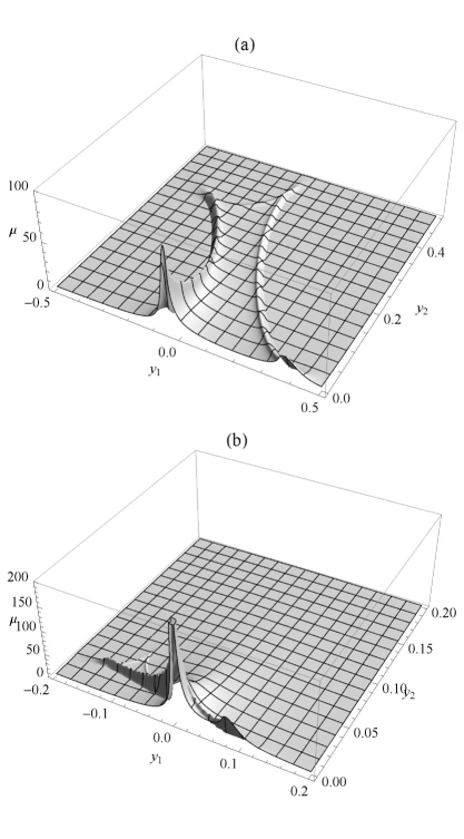
Figure 2: (a) Magnification map for a binary lens with mass ratio $q=0.1$ and separation $d=0.95$; the source radius is $\rho_{*}=0.01$; the step is $\Delta y_{1,2}=0.0025$. (b) Magnification map for a binary lens with mass ratio $q=0.001$ and separation $d=0.95$; the source radius is $\rho_{*}=0.001$; the step is $\Delta y_{1,2}=0.001$.

6 Numerical examples

In this section we will consider some explicit examples of magnification computations with the aim of illustrating the power of the innovations proposed in the previous sections.

6.1 Testing the error estimate

In order to present a test as exhaustive as possible, we calculate magnification maps with different levels of target accuracy $\delta\mu$ and evaluate the relative difference. We take maps calculated at $\delta\mu=10^{-5}$ as reference maps. Maps calculated at $\delta\mu=10^{-2}$ should not deviate from the reference maps by more than $10^{-2}$ in order to declare our error estimate successful. On the other hand, we do not want the deviation to be too small either, because this would mean that we are making more calculations than required for matching our target accuracy. In this subsection we are not considering limb darkening because we want to focus on the accuracy of the single contour calculation.

As a first example, we shall consider a binary lens with mass ratio $q=0.1$ and separation $d=0.95$ (intermediate caustic topology). Fig. 2a shows the reference magnification map obtained with a source radius $\rho_{*}=0.01$ and a step size $\Delta y=0.0025$ on the source plane in both directions. The caustic is very clearly visible, with a spike in the $\vec{y}=0$ position, where we get the maximum magnification.

As a second example, we consider a planetary lens with $q=0.001$ and $d=0.95$ (resonant caustic topology). We choose the resonant caustic topology since it corresponds to the maximum caustic extension, allowing finer and more stringent tests. The reference map for $\rho_{*}=0.001$ and $\Delta y=0.001$ is shown in Fig. 2b. The central spike is much higher in this case, because the source radius is much smaller (which is necessary for a better probing of the caustic).

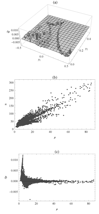
Figure 3: (a) Map of the errors for a binary lens with mass ratio $q=0.1$ and separation $d=0.95$; the source radius is $\rho_{*}=0.01$; the target accuracy is $\delta\mu=10^{-2}$. (b) Number of points used in sampling vs magnification. (c) Matched accuracy vs magnification.

Now, let us come to the first test. In Fig. 3a we show the magnification difference map between a map calculated at $\delta\mu=10^{-2}$ and the reference map shown in Fig. 2a. We can note that deviations tend to be spatially correlated far from the caustic, while they are very noisy at caustic crossings. However, as it is evident from Fig. 3c, the target accuracy is fully achieved by all points in the magnification map. There are just six points with $\delta\mu>10^{-2}$, with the maximum error being $\delta\mu=0.012$. We can consider this number of points with slightly exceeding error acceptable. We can also note that higher magnification points in the map tend to have smaller errors, with deviations staying one order of magnitude less than the required accuracy. Without the parabolic correction and the exit prescription described at the end of Section 4, the discrepancy between the errors of low and high magnification points would be much higher, so we consider this as a good result of our error estimate strategy. We can barely see something like a damped oscillatory behavior of the plot as a function of the magnification. Finally, in Fig. 3b we plot the number of sampling points versus the magnification. The number of sampling points needed for matching a fixed accuracy $\delta\mu$ grows almost linearly with magnification, which is what we expect in a Green’s theorem approach.

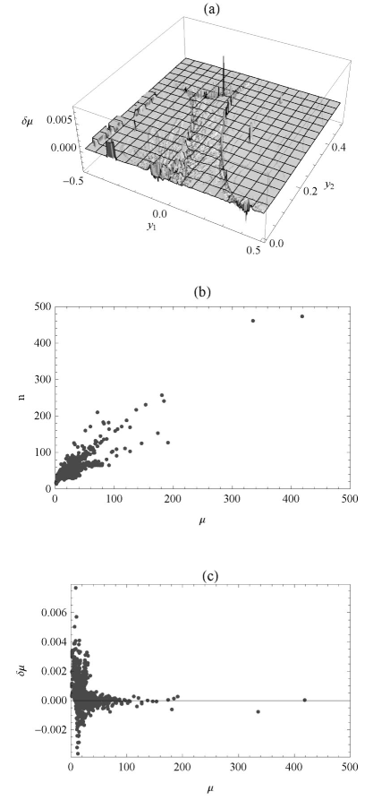
Figure 4: Same as Fig. 3 with a source radius $\rho_{*}=0.001$.

Reducing the source size from $\rho_{*}=0.01$ to $\rho_{*}=0.001$ has a slightly beneficial effects on the errors, which however stay at the correct order of magnitude, as we can see from Fig. 4.

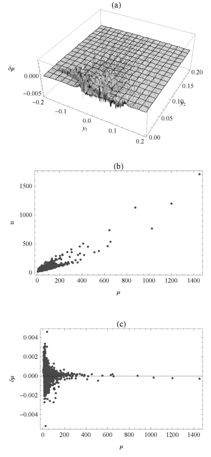
Figure 5: Same as Fig. 3 with a source radius $\rho_{*}=0.001$ and a planetary mass ratio $q=0.001$.

Coming to the planetary lens, the error map is shown in Fig. 5a, where errors appear much more scattered and less concentrated on the caustic. The errors stay at the correct order of magnitude and everything seems to be very stable with respect to the mass ratio.

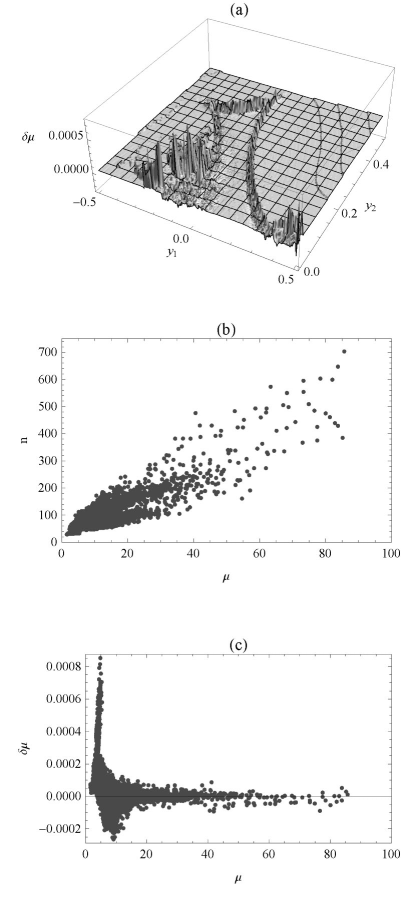
Figure 6: Same as Fig. 3 with a target accuracy $\delta\mu=10^{-3}$.

Finally, we come back to the mass ratio $q=0.1$ and $\rho_{*}=0.01$ and try a map with higher target accuracy $\delta\mu=10^{-3}$. Fig. 6 shows that our sampling strategy and our error estimate performs in a very successful way at any target accuracy, with all deviations having the correct order of magnitude.

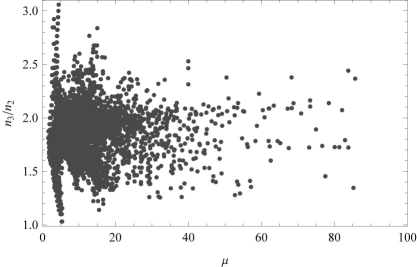
Figure 7: Ratio of the number of sampling points for an accuracy $\delta\mu=10^{-3}$ and the number of sampling points with $\delta_{\mu}=10^{-2}$. The ratio is plotted versus the magnification.

Since the plots of Fig. 3 and 6 only differ for the target accuracy, it is interesting to see how many sampling points we need to add to go from $\delta\mu=10^{-2}$ to $\delta\mu=10^{-3}$. In Fig. 7 we plot the ratio between the number $n_{3}$ of sampling points with $\delta\mu=10^{-3}$ and the number $n_{2}$ of sampling points with $\delta\mu=10^{-2}$ versus the magnification. Firstly, we see that the ratio does not depend on the magnification. Secondly, we can see that the number of sampling points is roughly doubled in order to increase the accuracy by a factor of 10. More precisely, the average factor $<n_{3}/n_{2}>=1.77$ in our maps. This can be understood analytically as follows. Considering that the residual error of the parabolic correction goes as $\Delta\theta^{5}$ but the number of sampling points in the interval $[0,2\pi]$ goes as $\Delta\theta^{-1}$, the accuracy in the magnification goes as $n^{-4}$. If $n$ is doubled, the accuracy is improved by a factor 16 (it would be just $n^{2}=4$ without the parabolic correction). With $<n_{3}/n_{2}>=1.77$ we have $<\delta\mu_{2}/\delta\mu_{3}>=<n_{3}/n_{2}>^{4}=9.81$, which is very close to the ratio of the target accuracies of the two maps.

6.2 Linear vs Parabolic approximation

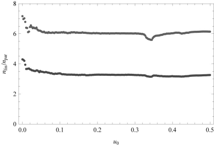
Figure 8: Speed-up due to the parabolic correction for microlensing trajectories parallel to the $y_{1}$ axis and $u_{0}$ varying from 0 to 0.5 (the reference map is in Fig. 2a). The upper points are for target accuracy $\delta\mu=10^{-3}$ and the lower points are for $\delta\mu=10^{-2}$.

In the previous subsection we have demonstrated that our error estimators give us a full control of the accuracy of our calculations. Now we can go into more detail and try to evaluate the speed-up due to the parabolic correction.

In order to give an estimate as realistic as possible, we should consider the calculation of typical microlensing light curves, i.e we should sum up the time spent for calculating the magnification along straight lines in the source plane. A good sample of straight lines is provided by the rows of our magnification maps. In fact, each row at constant $y_{2}$ can be considered as a straight source trajectory parallel to the $y_{1}$ axis with impact parameter $u_{0}=y_{2}$. Let us denote the number of sampling points on each row by $n_{par}(u_{0})$. This number is proportional to the total time spent for calculating the full row at $y_{2}=u_{0}$.

Similarly, we shall denote the number of sampling points in the analogous linear calculation (without the parabolic correction) by $n_{lin}(u_{0})$. In order to compare analogous calculations, the target accuracy $\delta\mu$ must be the same in both cases. As error estimator in the linear case, we use the parabolic correction itself, which is already available in our code.

The ratio $n_{lin}/n_{par}$ is thus a measure of the speed-up obtained by the introduction of the parabolic correction. Fig. 8 shows this quantity as a function of $u_{0}$ for a target accuracy of $\delta\mu=10^{-3}$ (upper points) and $\delta\mu=10^{-2}$ (lower points). The number of sampling points drops by a factor 3.3 in average for $\delta\mu=10^{-2}$ and 6.1 for $\delta\mu=10^{-3}$. The speed-up is even higher for central events with $u_{0}\simeq 0$, in which high-magnification points have a considerable weight. Such numbers are very encouraging, since a factor 6 may bring the computational time e.g. for a huge Markov chain from one weak to a single day.

6.3 Uniform vs Optimal sampling

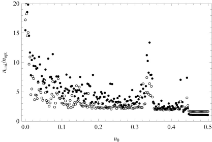
Figure 9: Speed-up due obtained thanks to optimal sampling for microlensing trajectories parallel to the $y_{1}$ axis and $u_{0}$ varying from 0 to 0.5 (the reference map is in Fig. 2a). Empty circles are for target accuracy $\delta\mu=10^{-2}$; filled circles are for $\delta\mu=10^{-3}$.

The next innovation proposed in this paper is the optimal sampling driven by a reliable estimate of the residual error in each arc between two sampling points. Indeed, by increasing the sampling only where really needed (e.g. close to caustic crossings of the source boundary), we expect to save a considerable amount of computational time.

In order to evaluate the speed-up, we adopt the same strategy explained in the previous subsection: we sum up the number of sampling points for each point in the magnification map at fixed $y_{2}$, so that we can have a measure of the time needed to calculate a microlensing light curve for a source trajectory parallel to the $y_{1}$ axis and with $u_{0}=y_{2}$. We denote the number of sampling points with the optimal sampling strategy by $n_{opt}$ and the number of sampling points with a uniform sampling by $n_{uni}$. The number of sampling points in the uniform case is determined by doubling the initial two-points sampling $\{0,\pi\}$ until the new magnification differs from the previous one by less than $\delta\mu/2$, where $\delta\mu$ is the target accuracy. Note that this prescription is sometimes unsafe, since we can have very small features in the images, which could be completely missed. However, for the purpose of a gross estimate of the speed-up, we adopt this prescription for the uniform sampling, since at most we are just underestimating the correct speed-up in some points.

In Fig. 9 we plot the ratio $n_{uni}/n_{opt}$ as a function of $u_{0}$ for trajectories parallel to the $y_{1}$ axis. The binary lensing geometry is that described in Fig. 2a. We can see that the speed-up reaches 20 for central trajectories and then falls down for larger impact parameters. Indeed, when the source is poorly magnified, there is no need for optimal sampling. The average speed-up is 3.3 for a target accuracy $\delta\mu=10^{-2}$ and 4.8 for $\delta\mu=10^{-3}$, though high magnification events get a much larger benefit from optimal sampling.

6.4 Limb Darkening

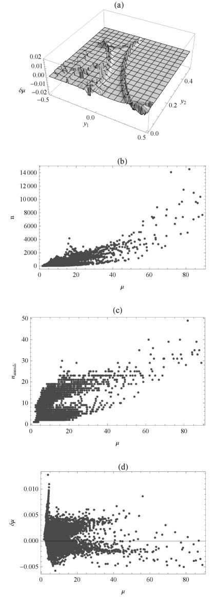
Figure 10: (a) Map of the errors for a binary lens with mass ratio $q=0.1$ and separation $d=0.95$; the source radius is $\rho_{*}=0.01$ with a linear limb darkening $a=0.51$; the target accuracy is $\delta\mu=10^{-2}$. (b) Number of points used in sampling vs magnification. (c) Number of annuli vs magnification. (d) Matched accuracy vs magnification.

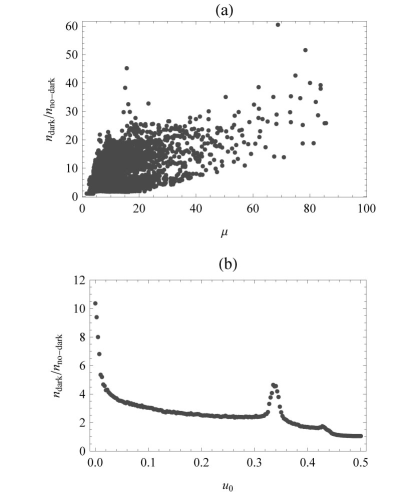
Figure 11: (a) Ratio between the number of points used with and without the limb darkening treatment. (b) Slow-down due to the limb darkening treatment for microlensing trajectories parallel to the $y_{1}$ axis and $u_{0}$ varying from 0 to 0.5.

As a final test of our code, we consider a linear limb darkened source with $a=0.51$ and radius $\rho_{*}=0.01$. We have generated a reference magnification map with target accuracy $\delta\mu=10^{-4}$. We do not show it because it looks very similar to Fig. 2a, except for the height of the magnification peaks. After that, we have generated a test magnification map with target accuracy $\delta\mu=10^{-2}$. In both cases we have used the error estimators introduced in section 5 and the optimal source sampling strategy described there.

The difference between the test and the reference map is shown in Fig. 10a. We can see that errors are kept well under control, in particular at caustic crossings, which represent the most crucial tests for limb darkening. Of course, approximating limb darkening by the contour method requires a large number of points. In Fig. 10b we have a plot of the number of sampling points (adding those in all annuli) vs the magnification. We can see that the number of points grows faster than linearly with magnification at large $\mu$. The number of annuli (Fig. 10c) grows rapidly from 1 to 20 at low magnifications and then stays more or less constant up to very high magnifications. Finally, Fig. 10d shows that the target accuracy has been achieved by all points save for three with $\delta\mu=0.011$.

The bottom line of our limb darkening code is the slow-down plot shown in Fig. 11. We compare the number of points required for a calculation of limb darkening by summing up the number of sampling points in all annuli. We denote this number by $n_{dark}$. We compare this number with the number of sampling points in the uniform source case ($n_{no-dark}$). In panel (a) we show the ratio $n_{dark}/n_{no-dark}$ vs the magnification. Furthermore, as in previous subsections, we sum up the total number of sampling points along each row at fixed $y_{2}$ in our magnification map. This is an indication of the total time spent for calculating a full microlensing trajectory parallel to the $y_{1}$ axis with $u_{0}=y_{2}$. The ratio of the number of points including the limb darkening treatment $n_{dark}$ and the number of points calculated for a uniform brightness disk $n_{no-dark}$ therefore represents the slow-down factor of our code for the inclusion of the limb darkening treatment. From Fig. 11b we see that the average slow-down factor is 2.64, but central trajectories may be slowed down to a factor of 11. Interestingly, we also have two peaks at impact parameters $u_{0}=0.34$ and $u_{0}=0.42$, which correspond to trajectories including cusp crossings.

7 Conclusions

In this paper we have presented four innovations for codes attempting microlensing calculations based on contour integration. In this class of codes the contours of the images are obtained by inversion of the lens map at the source boundary; the area of the images is then obtained by a simple contour integration rather than by a surface integration.

We have introduced a parabolic third order correction in the evaluation of Green’s line integral, which leaves a residual of the fifth order in the interval size $\Delta\theta$. The speed-up with respect to the classical trapezium approximation is around 4 for a target accuracy in the magnification of $\delta\mu=10^{-2}$.

We have introduced accurate error estimators, whose reliability has been shown by comparing several magnification maps obtained at different levels of target accuracy.

Thanks to these error estimators, we have proposed a new optimal sampling strategy driven by the error estimates in each sampling interval. With respect to a uniform sampling we get a speed-up ranging from 3 to 20 at $\delta\mu=10^{-2}$ depending on how large is the magnification experienced by the source in its microlensing trajectory.

Finally, we have faced the problem of limb darkening, which is the hardest obstacle for codes based on contour integration. Also in this case we have introduced error estimators and an optimal sampling strategy with the aim of minimizing calculation keeping full control of the accuracy. As a result, we have a very reliable limb darkening approximation to any desired accuracy. At $\delta\mu=10^{-2}$ the slow-down with respect to a uniform brightness disk ranges from 2 to 11.

Summing up, the speed-up gained by the optimal sampling is sufficient to compensate the slow-down due to the migration from uniform brightness disks to realistic limb darkened sources. In addition, the parabolic correction guarantees a net speed-up with respect to traditional linear Green’s theorem codes. Finally, the full control of the errors is an invaluable help in order to avoid redundant calculations and concentrate the efforts where it is really needed. Its impact with respect to traditional codes with fixed sampling is definitely huge and difficult to quantify.

All these innovations should put codes based on contour integration in the front line for binary and planetary microlensing events modelling.

References

- Bealieu et al. (2006) Beaulieu J.-P. et al., 2006, Nature, 439, 437
- Bennett (2009) Bennett D.P., 2009, arXiv:0911.2703
- Bennett & Rhie (1996) Bennett D.P., Rhie S.H., 1996, ApJ, 472, 660
- Bennett et al. (2004) Bennett D.P. et al., 2008, ApJ, 684, 663
- Bond et al. (2004) Bond I. et al., 2004, ApJ, 606, L155
- Dominik (1993) Dominik M., 1993, Effiziente Methoden zur Invertierung der Gravitationslinsengleichung und zur Analyse von Bildern ausgedehnter Quellen, Diploma thesis, Universität Dortmund.
- Dominik (1995) Dominik M., 1995, A&AS 109, 507.
- Dominik (1998) Dominik M., 1998, A&A 333, L79.
- Dominik (2007) Dominik M., 2007, MNRAS, 377, 1679
- Dominik (2010) Dominik M., 2010, to appear on Gen. Rel. and Grav., DOI: 10.1007/s10714-010-0930-7.
- Dong et al. (2006) Dong S. et al., 2006, ApJ, 642, 842
- Dong et al. (2009) Dong S. et al., 2009, ApJ, 698, 1826
- Gaudi (2010) Gaudi B.S., 2010, arXiv:1002.0332
- Gaudi et al. (2008) Gaudi B. S., et al., 2008, Science, 319, 927
- Gould (2008) Gould A., 2008, ApJ, 681, 1593
- Gould & Gaucherel (1997) Gould A., Gaucherel C., 1997, ApJ, 477, 580
- Gould et al. (2006) Gould A., et al., 2006, ApJ, 644, L37
- Gould & Loeb (1992) Gould A., Loeb A., 1992, ApJ, 396, 104
- Janczak et al. (2009) Janczak J. et al., 2009, arXiv:0908.0529
- Kayser et al. (1986) Kayser R., Refsdal S., Stabell R., 1986, A&A, 166, 36
- Mao & Paczyński (1991) Mao S., Paczyński B., 1991, ApJ, 374, 37
- Milne (1921) Milne E.A., 1921, MNRAS, 81, 361
- Paczyński (1986) Paczyński B., 1986, ApJ, 304, 1
- Pejcha O. & Heyrovský (2009) Pejcha O., Heyrovský D., 2009, ApJ, 690, 1772
- Press et al. (2007) Press W.H. et al., 2007, ”Numerical Recipes 3rd Edition: The Art of Scientific Computing”, Cambridge University Press.
- Rattenbury et al. (2002) Rattenbury N.J., Bond I.A., Skuljan J., Yock P.C.M., 2002, MNRAS, 335, 159
- Schneider et al. (1992) Schneider P., Ehlers J., Falco E.E., 1992, ”Gravitational lenses”, Springer-Verlag, Berlin.
- Schramm & Kayser (1987) Schramm T., Kayser R., 1987, A&A 174, 361.
- Sumi et al. (2010) Sumi T. et al., 2010, ApJ, 710, 1641
- Udalski et al. (2005) Udalski A. et al., 2005, ApJ, 628, L109
- Wambsganss (1997) Wambsganss T. R., 1997, MNRAS, 284, 172
- Witt (1990) Witt H. J., 1990, A&A, 236, 311