Waldmeier Effect in Stellar Cycles

Abstract

One of the most robust features of the solar magnetic cycle is that the stronger cycles rise faster than the weaker ones. This is popularly known as the Waldmeier Effect, which is known for more than 80 years. This fundamental feature of the solar cycle has not only practical implications, e,g., in predicting the solar cycle, but also implications in understanding the solar dynamo. Here we ask the question whether the Waldmeier Effect exists in other Sun-like stars. To answer this question, we analyze the Ca ii H & K S-index from Mount Wilson Observatory for 21 Sun-like G–K stars. We specifically check two aspects of Waldmeier Effect, namely, WE1: the anti-correlation between the rise times and the peaks and WE2: the positive correlation between rise rates and amplitudes. We show that except HD 16160, HD 81809, HD 155886 and HD 161239, all stars considered in the analysis show WE2. While WE1 is found to be present only in some of the stars studied. Further, the WE1 correlation is weaker than the WE2. Both WE1 and WE2 exist in the solar S-index as well. Similar to the solar cycles, the magnetic cycles of many stars are asymmetric about their maxima. The existence of the Waldmeier Effect and asymmetric cycles in Sun-like stars suggests that the dynamo mechanism which operates in the Sun is also operating in other stars.

1. Introduction

The solar magnetic activity increases and decreases cyclically with an average period of 11 years, however, both the duration and amplitude vary cycle to cycle. There are also short-term variations within the cycle (Lean and Brueckner, 1989), making it difficult to predict the future activity. Nonetheless, there are some special features of the solar cycle. One of these is that the rate of increase of the activity is not the same for all cycles, rather it depends on the strength of the cycle. This leads to a famous relation, called the Waldmeier Effect (Waldmeier, 1935). It says that the stronger cycles rise faster (and take less time to reach their peak activities) than the weaker ones, and vice-versa. The Waldmeier Effect has been extensively studied in different proxies of solar activity data since its discovery in 1935. However, limitations in different data sets sometimes make it difficult to establish its existence. For example, Dikpati et al. (2008) did not find a significant anti-correlation between rise times and amplitudes and claimed that the Waldmeier Effect is not present in the sunspot area data. Later, a more careful analysis by Karak and Choudhuri (2011) computed the rise time and showed that Waldmeier Effect exists in all, sunspot area, number and 10.7-cm radio flux data. They further showed that this anti-correlation between rise times and amplitudes is one aspect of Waldmeier Effect which they referred to as WE1. The other aspect is the positive correlation between the rise rates and the amplitudes and they referred to it as WE2. It turned out that the latter feature is much more robust and probably more useful (Cameron and Schüssler, 2008). For example, when the Waldmeier Effect is used to predict the future solar cycle, WE2 is meant rather than WE1 which requires rise time of the cycle (e.g., Cameron and Schüssler, 2007; Kane, 2008; Ramesh and Lakshmi, 2012). Only after the cycle has reached its maximum can the rise time be obtained while the rise rate can easily be obtained shortly after the cycle has started.

Many other stars, so-called the Sun-like stars (with spectral types F–M), which have convection zones in their outer layers produce magnetic fields through dynamo action (Parker, 1955; Moffatt, 1978; Gilman, 1983; Ossendrijver, 2003; Charbonneau, 2014; Noyes et al., 1984; Soon et al., 1993; Saar and Brandenburg, 1999). Many of these stars indeed show clear magnetic cycles with varying amplitudes and durations (Baliunas et al., 1995). Therefore, the important question that we want to answer in this paper is whether the Waldmeier Effect can be seen in other stars as well. Checking the Waldmeier Effect in other stars, however, is challenging because typically we do not have a long dataset of magnetic activity. Among the available observables of magnetic activity, Ca ii H & K line emission (hereafter simply HK) is the longest dataset that has been used to study the long-term variation of stellar activity. The magnetic (non-thermal) heating in the chromosphere causes emission in the cores of HK. This HK emission is used to measure the stellar magnetic activity due to its strong correlation with the magnetic flux, as realized in the Sun (Leighton, 1959; Skumanich et al., 1975; Schrijver et al., 1992).

The HK Project of Mount Wilson Observatory (MWO) regularly monitored more than 100 Sun-like stars with spectral types early F to M, starting from 1966. However, the Project ended in 2003. Therefore, this limited data of 37 years may be used to analyze the features of stellar cycles. Analyzing these data from 21 stars for which good cycles are seen, we shall explore the existence of Waldmeier Effect in different Sun-like stars for the first time. Other features of stellar cycles, particularly the asymmetry of the cycles will also be identified. To put the Sun in this context, we shall also present the analysis of Waldmeier Effect using the same Ca ii HK proxy obtained from Kodaikanal Observatory, which was not done in the past.

Figure 1.— Stellar cycles used in our analysis. Dotted points are the MWO’s calibrated S-index, while solid blue and dashed red lines are the fitted data using skewed-Gaussian and quasi-Planck functions, respectively.

Figure 2.— Same as Figure 1 but for the Sun. Left panel: Kodaikanal Observatory data and right: MWO data scaled; see Egeland et al. (2017) for details.

2. Data Analyses

We use the fully calibrated S-index time series from the MWO HK Project. In our analysis we need high-quality data having at least two consecutive unambiguous cycles. These are available only in G and K stars which are also listed in Böhm-Vitense (2007) and Schröder et al. (2013). From these lists, we find that only 21 stars are useful in our study. Chromospheric variations of these stars are shown in Figure 1, while the cycle properties are listed in Table 1. The dotted points in this figure show the raw data, the calibrated S-index. The S-index for the Sun, obtained from the Kodaikanal Observatory is also shown for comparison in Figure 2.

To study the Waldmeier Effect using these S-index data, we need to compute the rise time, rise rate, and peak value of each cycle. However, as can be seen from Figure 1, the data are irregular (due to the rotation, active region emergence and decay, and uneven observations). Thus, we end up getting huge uncertainties in the cycle parameters if they are computed directly from the calibrated S-index. Therefore, instead of using the raw calibrated S-index data, we produce approximate cycles of the data using the given profile(s) and then the best-fitted cycles are used to study the Waldmeier Effect. What profile we use to produce the fitted data is guided by the fitting of solar data. A popular fitting profile of the solar cycle is the following quasi-Planck function (Hathaway et al., 1994).

$$f(t)=\frac{a(t-t_{0})^{3}}{\exp\left[\frac{(t-t_{0})^{2}}{b^{2}}\right]-c},$$ (1)

where $t$ is the time in year, $t_{\rm 0}$ is the starting time of the cycle, parameters $a$, $b$ and $c$ are related to the cycle amplitude (peak S-index), the rise time, and the cycle asymmetry, respectively. On the other hand, Du (2011) has demonstrated that the following skewed-Gaussian function captures the solar cycle profile slightly better.

$$f(t)=A\exp\left[\frac{-(t-t_{m})^{2}}{2B^{2}[1+\alpha(t-t_{m})]^{2}}\right]+f_{\mathrm{min}},$$ (2)

where $A$ is related to the cycle amplitude, $t_{\rm m}$ is approximately the time of maximum, $B$ relates to the width of the cycle rising phase, and $\alpha$ is the asymmetry parameter. The last term $f_{\rm min}$, which measures the offset S-index at the cycle minimum, was not present in the Du (2011) model, but was introduced recently by Egeland et al. (2017). Although they preferred this profile, they have shown the fitting with the quasi-Planck function produces comparable results. We, therefore, fit the stellar S-index with both profiles and study the Waldmeier Effect separately in each fitted data.

As the fitting will be performed for each cycle separately, we need to isolate the cycles first. To do so, we bin the raw data with one-year intervals and then smooth with a three-point running window. In this smoothed S-index, the cycles are isolated by considering the data in between two successive minima. The individual cycle periods computed from two successive minima and their mean periods for all stars are enlisted in the last two columns of Table 1. Taking the minimum time as a heuristic value, we proceed to fit the raw S-index of individual cycles with functions given in equations (1) and (2). For the fitting, we use the Python scipy library curve_fit routine. This built-in function uses a Trusted Region Reflective (TRR) method with the Levenberg–Marquardt (LM) algorithm applied to trusted-region subproblems (Moré, 1978, p. 105). In Figures 1 and 2, the solid and dashed lines show the fitted profiles using skewed-Gaussian (Equation (2)) and quasi-Planck function (Equation (1)), respectively. To measure a goodness of fit we compute the reduced $\chi^{2}_{\rm red}$. In evaluating $\chi^{2}_{\rm red}$, we consider the error as $1.2\%$ of the S-index as suggested in Baliunas et al. (1995). Tables 3 and 4 in Appendix A list out the values of various fitted parameters and $\chi^{2}_{\rm red}$ for each of the stars used in the analysis. While for most stars these $\chi^{2}_{\rm red}$ values are reasonable considering that the models do not address short-timescale variability present in the data, we get significantly large values for a few stars where even the long-term variability appears to be not well represented by the models. While for some stars these $\chi^{2}_{\rm red}$ values are reasonable, we get significantly large values for a few stars which are due to poor data quality. We further observe that the $c$ column for quasi-Planck fit contains some extreme negative values. As such, although the trend is seen in general for most of the stellar cycles, it cannot be said that the parameter $c$ corresponds to the cycle asymmetry. It can also be seen that the parameter $t_{0}$ does not increase monotonically in every consecutive cycle of a star. Thus, the correspondence between $t_{0}$ and the cycle start time is also not thorough.

Sadly, not all the cycles are usable for the analysis. The observational data of most of the stars contains a partial cycle either initially or at the end of the observation period. These partial cycles cannot be used. Further, some cycles of HD 155885, HD 155886 and HD 201092 are unusable because of ill-fitting or inconsistent variability. Table 4 of Appendix A lists out the parameters values for such unusable cycles, whereas Table 3 gives the values for the usable cycles. The plots in Figure 1 can be reproduced from equations (1) and (2) using the parameters given in Table 3 and Table 4. To compare the goodness of the fitting of different stars we further compute $\chi^{2}_{\rm red}$ for all the usable cycles in each star. This total $\chi^{2}_{\rm red}$ is shown in Table 1. For the solar cycles, we get $\chi^{2}_{\rm red}$ values as 3.5 for quasi-Planck and 2.5 for skewed-Gaussian fittings.

We note that the observational data of the stellar magnetic activity sometimes contains local minima between the cycles. We ignore the local minima when the time difference between the minimum and the preceding maximum is much less compared to such difference for other cycles. The threshold value of the time difference for this criterion of ignoring the local minima varies from star to star and depends on the cycle characteristics. For instance, for HD 201092, the local minima are ignored if the time interval containing the minimum is $\sim 3$ years or less. Whereas, in the case of HD 149661, since the actual cycle durations are in that range, we do the same for a much smaller interval ($\sim 1$ years).

Further, another important parameter to look into is the cycle asymmetry. Solar magnetic cycles are usually found to be asymmetric about the maxima. Therefore it is interesting to find out whether the stellar cycles are also asymmetric. A measure of this asymmetry in the cycle can be obtained by calculating the skewness of the data defined as

$$\gamma_{1}=\frac{\sum_{i=1}^{N}(f^{d}_{i}-\bar{f})^{3}}{(N-1)\,\sigma_{fit}^{3}},$$ (3)

where $\bar{f}$ is the mean strength of the cycle and $\sigma_{\rm fit}$ is the standard deviation of the cycle data from the fitted profile. Column 7 of Table 1 tabulates the mean value of the skewness for the stars $\overline{\gamma_{1}}$, calculated using the individual skewness values of usable cycles. A positive (negative) skewness means that the part of the cycle on the right (left) of the cycle maxima is skewed compared to the other side. For reference, the mean skewness of the solar cycles computed from our S-index is $0.3373$.

Table 1Summary of data analysis and results.

Star	SpecType	Data duration	# cycles	$\chi^{2}_{\rm red,P}$	$\chi^{2}_{\rm red,G}$	$\overline{\gamma_{1}}~{}~{}$	WE1?	WE2?	$P_{\rm cyc}\rm{(yr)}$	$P_{\rm cyc}^{\rm mean}\rm{(yr)}$
HD 3651	K0V	1966–2002	2	12.6	11.0	2.26	WE1G	WE2G	13.81, 15.99	14.90
HD 4628	K2V	1966–2002	3	20.5	11.6	0.60	WE1P,G	WE2P,G	8.67, 8.08, 9.98	8.91
HD 10476	K1V	1966–2002	3	16.5	10.7	0.85	No	WE2P,G	10.50, 10.57, 10.61	10.56
HD 16160	K3V	1967–2002	2	18.6	17.8	0.00	WE1G	No	10.99, 14.31	12.65
HD 20630	G5V	1967–2002	3	11.0	9.5	0.10	WE1G	WE2P,G	4.83, 5.50, 7.21	5.85
HD 26965	K1V	1967–2002	3	8.9	8.8	0.02	No	WE2P,G	10.08, 9.58, 8.96	9.54
HD 32147	K3+V	1967–2002	2	21.2	19.2	0.08	WE1P,G	WE2P,G	9.33, 12.42	10.88
HD ${81809}^{{\dagger}}$	G2IV+G2V	1966–2002	4	9.8	8.4	0.14	No	No	7.96, 8.74, 6.50, 7.32	7.64
HD 103095	KV	1968–2002	4	9.1	8.2	0.50	No	WE2P,G	6.58, 7.50, 6.58, 6.90	6.89
HD 115404	K2.5V	1968–2002	2	25.8	25.4	$-0.19$	WE1P,G	WE2G	11.99, 8.84	10.42
HD 149661	K0V	1967–2002	7	23.0	20.6	0.34	No	WE2P,G	3.95, 3.54, 4.84, 3.75, 6.42, 5.34, 4.46	4.61
HD 152391	K8+V	1966–2002	3	28.7	24.6	$-0.15$	WE1G	WE2P,G	11.16, 9.83, 8.10	9.70
HD 155885	K1V	1967–2002	4	29.3	19.7	0.30	No	WE2P	5.08, 5.67, 6.19, 1.47	4.60
HD 155886	K2V	1967–2002	2	25.4	23.7	0.30	WE1P	No	7.33, 5.99	6.67
HD 156026	K5V	1966–2002	2	75.3	74.1	$-0.58$	No	WE2P	17.16, 8.87	13.02
HD 160346	K2.5V	1966–2002	4	28.2	16.4	0.22	No	WE2P,G	7.58, 7.58, 7.13, 6.45	7.19
HD 161239	G2IIIb	1966–2001	5	8.0	7.6	0.55	No	No	14.17, 5.17, 4.67, 5.17, 4.29	6.69
HD 166620	K2V	1966–2002	2	22.4	17.4	5.99	WE1P,G	WE2G	17.08, 11.59	14.34
HD 201091	K5V	1967–2002	4	27.7	28.5	0.39	No	WE2P,G	7.42, 8.08, 6.50, 6.52	7.13
HD 201092	K7V	1967–2002	3	56.9	39.6	$-0.07$	No	WE2P	4.76, 10.58, 5.32	6.89
HD 219834B	K2V	1967–2002	4	50.5	38.0	0.36	WE1G	WE2P,G	8.10, 11.25, 8.92, 5.47	8.45
Sun	G2V	1913–2016	10	3.5	2.5	0.34	WE1P,G	WE2P,G	7.84–11.49	10.35

3. Results

3.1. Checking the Waldmeier Effect in solar S-index

As referred in the Introduction that previous authors have studied the Waldmeier Effect using sunspot number and area data, but not using any chromospheric magnetic proxy. Therefore, we shall first check the Waldmeier Effect for the Sun with the same type of chromospheric magnetic proxy that we are using for the other stars. This will show the robustness of our analysis and also put the Sun in the stellar context. For this, we use the S-index of Sun from MWO data for the last 5 cycles and Kodaikanal data where the data is available for cycles 15–19. As described in Egeland et al. (2017), these two data sets are made homogeneous by doing the following scaling.

Figure 3.— Left: scatter plots for WE2 (positive correlation between rise rates and the amplitudes). Right: WE1 (anti-correlation between rise times and amplitudes) for the solar Cycles. Top and bottom panels obtained from quasi-Planck and skewed-Gaussian fitted data, respectively. The solid lines are linear fits with slopes $m=0.030\pm 0.023$, $0.032\pm 0.022$, $-0.033\pm 0.062$ & $-0.045\pm 0.064$ and intercepts $c=0.970\pm 0.025$, $0.968\pm 0.024$ , $1.033\pm 0.063$ & $1.046\pm 0.065$, with the rms-deviation of fittings being $0.011$, $0.013$, $0.014$ & $0.018$, respectively for panels a, b, c and d.

The Kodaikanal data is in Integrated Sunlight Spectrometer (ISS) flux scale, calibrated by Bertello et al. (2016) using the synoptic Ca ii K plage index from spectroheliograms from the Kodaikanal (KKL) Observatory in India. This time series data of Ca ii K emission is first transformed to the Ca ii H & K measurement scale of Sacramento Peak National Observatory (NSO/SP) flux scale by applying following equation.

$$K_{\rm KKL(SP)}=1.1388K_{\rm KKL(ISS)}-0.0071.$$ (4)

Now, another transformation is performed between the NSO/SP K emission index and the MWO S-index. Assuming a linear relationship of the form, $S(K)=a+bK$, and using the cycle 23 fit parameters for the Sun (Egeland et al. (2017)), the following linear transformation is obtained:

$$S(K)=(1.5\pm 0.13)K+(0.031\pm 0.013)$$ (5)

Using Equation (5) for the Kodaikanal data between cycles 15–19, homogenizes the solar data.

Previous studies have shown that the WE2 (anti-correlation between rise rates and amplitudes) is a robust feature of the solar cycle. Therefore, we analyze the WE2 first using the data obtained from the quasi-Planck fitting. Following Karak and Choudhuri (2011), we define the rise rate of a cycle as the change in the activity in a single year and calculating the change between two consecutive years after leaving out one year from the cycle beginning (minimum). The scatter plot between the rise rate and the peak S-index is shown in the left panel of Figure 3 both for the quasi-Planck and skewed-Gaussian fittings. We find that the correlation is good and the value of the correlation coefficient is comparable to the previous study (Cameron and Schüssler, 2008; Karak and Choudhuri, 2011).

Now, we consider WE1 which is the anti-correlation between the rise time and the strength. As argued in Dikpati et al. (2008) and Karak and Choudhuri (2011), incorrect identification of cycle minimum or maximum can lead to a large error in the rise time computed. We, therefore, consider the rise time as the time taken by a cycle to grow from $20\%$ to $80\%$ of its peak. The scatter plot between the rise time and the peak S-index is shown in the right panel of Figure 3. As found in the other proxies of the solar cycle, the WE1 correlation is much weaker. The correlation coefficients found in our S-index data is comparable to the previous values obtained from other proxies of the solar data (Dikpati et al., 2008; Karak and Choudhuri, 2011).

Figure 4.— WE2 obtained from the quasi-Planck fitted S-index data of stars HD 160346 (left) and HD 201091 (right).

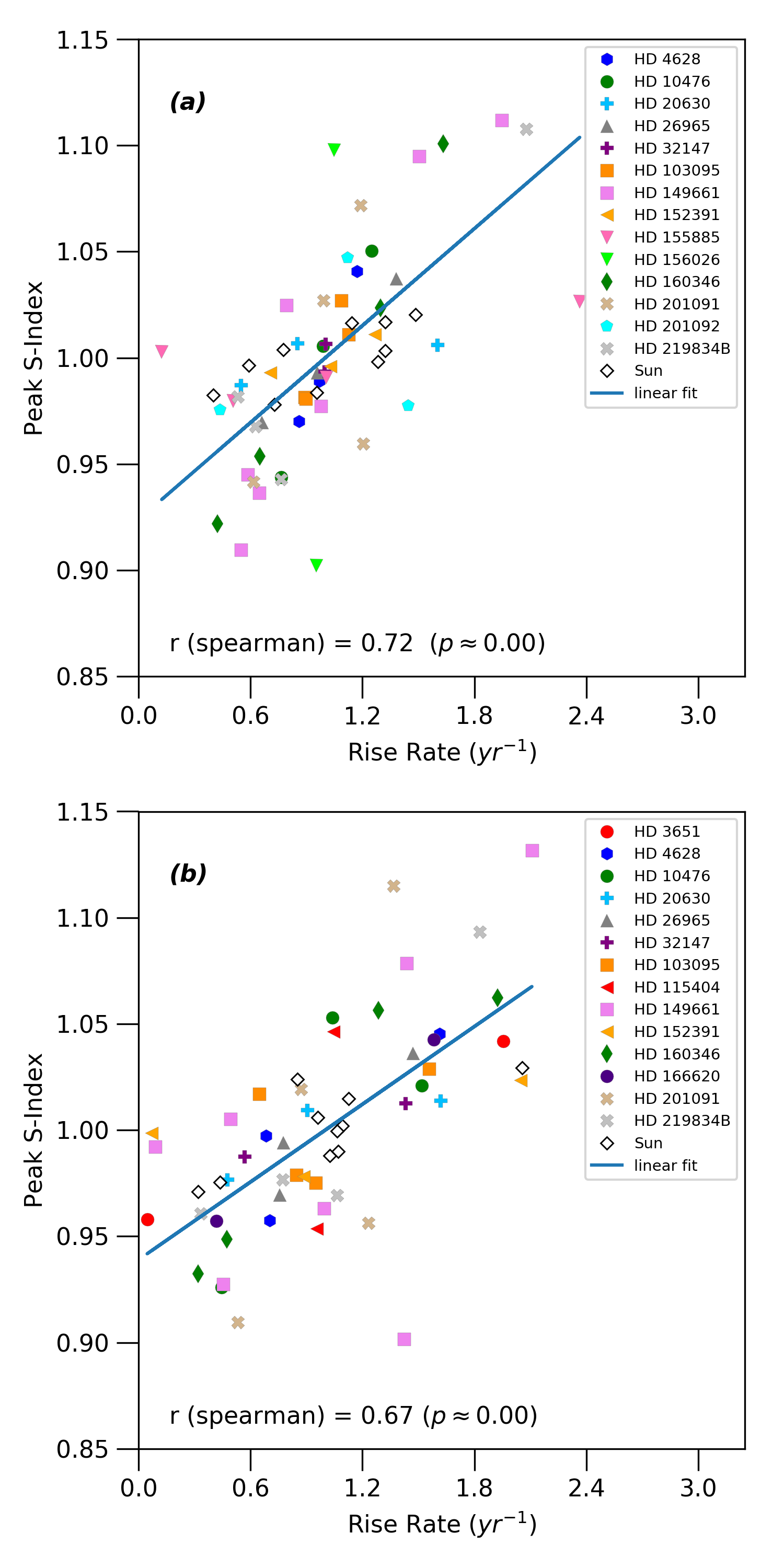
Figure 5.— Combined scatter plot for WE2. Different symbols represent different stars. The linear Spearman correlation and confidence level are printed on each plot. Top and bottom panels obtained from quasi-Planck and skewed-Gaussian fitted data. We note that the data of stars HD 16160, HD 81809, HD 155886, and HD 161239 are not included because these stars do not show a positive correlation. The solid lines are best linear fits with slopes $m=0.076\pm 0.025$ & $0.061\pm 0.021$ and intercepts $c=0.924\pm 0.028$ & $0.939\pm 0.024$, with the rms-deviation of fittings being $0.038$ & $0.039$, respectively for top and bottom panels.

3.2. Checking the Waldmeier Effect in Stars

Now we study the Waldmeier Effect for the stars in the same way as we have done for the Sun. We first show the results of WE2 using the data obtained from the quasi-Planck fitting. For the representation, the scatter plots between the rise rates and the peak S-indexes for HD 160346 and HD 201091 are shown in Figure 4. This shows that the stronger cycles rise faster than the weaker ones—establishing the WE2 in these two stars. As the number of cycles in each star is very limited, the correlation coefficient computed from the cycles of an individual star is not very meaningful. Therefore, we combine the data for all the stars which individually show the correlation for WE2. For a star, if the Spearman correlation coefficient between rise rates and amplitudes is at least $0.1$, then we mark that star to ‘hold WE2’. This information is listed in Table 1. Table 5 in Appendix A details the peak S–index and rise rate values for all the stars used in the analysis. Surprisingly, we find that all the stars except HD 16160, HD 81809, HD 155886 and HD 161239, follow WE2 for at least one type of fitting.

For HD 16160, there are only two cycles (see Figure 1). Therefore, with this limited data, it is difficult to make a conclusive comment about whether HD 16160 truly does not follow WE2. The same argument may hold for HD 155886 because this star also has only two usable cycles and both cycles are very noisy. In HD 161239, the correlation is destroyed due to the first cycle which is very different than the rest. As seen in Figure 1, for HD 161239, the first cycle is the strongest one and the activity level during the minimum is relatively high. This produces an unexpectedly slow rise rate in the first cycle and breaks the WE2 relation. If we do not consider the first cycle, then the star beautifully show WE2 (The linear Spearman correlation is $0.80$ for quasi-Planck fitted data and $0.20$ for skewed-Gaussian fitting). In the case of HD 81809, the cycles are very regular and the data quality is good. However, it is very surprising that the star does not follow WE2. The individual Spearman correlation coefficient between the rise rates and the amplitudes is $-0.80$ for the quasi-Planck fitting and $-0.40$ for the skewed-Gaussian. Thus the correlation is opposite to the one we expect for the WE2 to hold.

The combined data of stars having a good positive correlation between the rise rate and the amplitude are shown in the top panel of Figure 5. We note that different stars have different activity levels and cycle growth rates. Thus, to put all values in a comparable range, we normalize the data of individual stars with their average values. This does not affect the value of the correlation coefficient of the combined data. For comparison, the data from the Sun is also shown in the same plot. As seen from the top panel of Figure 5, the composite data show a good correlation between rise rates and strengths; excluding the solar data, the linear Spearman correlation coefficient being $0.72$. The data obtained from the skewed-Gaussian fitting show a similar behavior, although the correlation coefficient is lower; see bottom panel of Figure 5. Interestingly, the skewed-Gaussian profile is fitting the data better than the quasi-Planck profile (less $\chi^{2}_{\rm red,G}$ values as seen from Table 1); however, the Waldmeier relation is relatively weaker.

Finally, we explore WE1 for stars. Again, we first check the trend between rise times and the peaks for each star separately. We say that a star shows WE1 if the Spearman correlation coefficient between peaks and rise times is less than $-0.1$. As listed in Table 1, not all stars show the expected negative correlation. We find that only five stars out of $21$ show WE1 for the quasi-Planck fitting. For the skewed-Gaussian fitting, four more stars show the solar-like WE1 correlation.

The scatter plots between rise times and peak S-index of all the stars showing WE1 individually are shown in Figure 6. For comparison, the data for the Sun are overplotted in the same figure. In this figure, we observe that the correlation coefficient is much weaker. Excluding the solar data, the linear Spearman correlation coefficient is $-0.77$ ($p=0.01$) for quasi-Planck fittings, while this value for skewed-Gaussian fitting is $-0.39$ ($p=0.07$). Note that in the latter case, the correlation is very less and thus the results are statistically insignificant. It is the HD 219834B which has a very poor WE1 correlation ($-0.02$) and reduces the composite correlation in Figure 6(b). If we exclude this star, then the correlation becomes $-0.52$ ($p=0.02$). Weaker correlation for WE1 is not surprising because it is already known from the study of solar data that WE1 is much weaker and it is sensitive to the data set in use as well as the computation of rise times (Dikpati et al., 2008; Karak and Choudhuri, 2011). Fortunately, if instead of defining rise time as the time taken by a cycle to grow from $20\%$ to $80\%$ of its peak, we define it using different values, then also we get a solar-like negative correlation for WE1 from those stars which show correlations in Figure 6; (see Table 2). However, the correlation values for skewed-Gaussian remain far lower than those for the quasi-Planck fit.

Let us discuss a consequence of WE2 relation. As shown in Figure 5, WE2 can be read as $S=m(\frac{dS}{dt})+S_{0}$. Now if we make a crude assumption: $\frac{dS}{dt}=\frac{S}{t}$, where $t$ is the total rise time, and if we also take the limit $\frac{m}{t}<1$ (which is the case in our data), then to a first order, we find: $S=(mS_{0})\frac{1}{t}+S_{0}$. This relation fits the data presented in Figure 6 (WE1) poorly (rms deviation of the fittings being $0.029$ and $0.037$ for quasi-Planck and skewed-Gaussian fitted data). Our correlation plot for WE1 has already a large scatter and thus we cannot conclusively reject this variation over the linear variation represented as WE1.

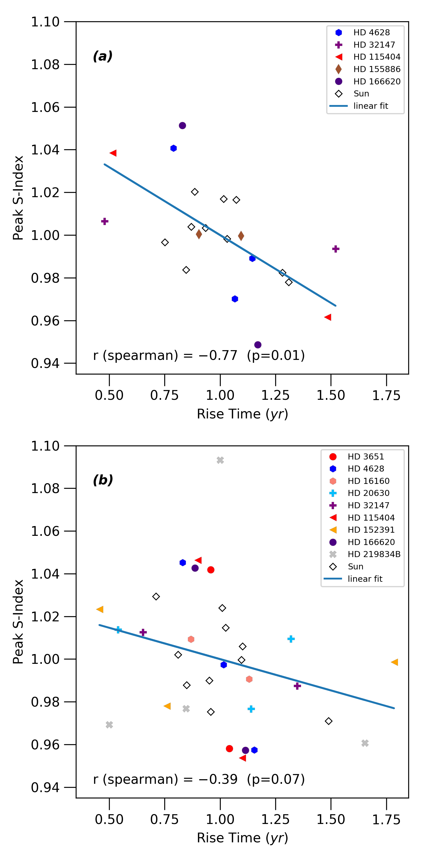
Figure 6.— Scatter plot for WE1. The figure format is same as Figure 5, however, in this case number of stars following solar-like WE1 is less. The solid lines are linear fits with slopes $m=-0.064\pm 0.055$ & $-0.029\pm 0.049$ and intercepts $c=1.064\pm 0.058$ & $1.029\pm 0.051$, with the rms-deviation of fittings being $0.026$ & $0.036$, respectively for top and bottom panels.

Table 2WE1 correlation coefficients

$t_{\rm start}$	$t_{\rm end}$	$r_{\rm Spearman}$
		quasi-Planck	skewed-Gaussian
0.15	0.75	$-0.80$	$-0.40$
0.15	0.80	$-0.81$	$-0.40$
0.15	0.85	$-0.78$	$-0.43$
0.20	0.75	$-0.80$	$-0.35$
0.20	0.80	$-0.77$	$-0.39$
0.20	0.85	$-0.75$	$-0.40$
0.25	0.75	$-0.82$	$-0.50$
0.25	0.80	$-0.81$	$-0.51$
0.25	0.85	$-0.81$	$-0.51$

4. Conclusion and Discussion

In this study, we for the first time have explored the Waldmeier Effect in Sun-like stars. We have used MWO’s calibrated S-index of $21$ stars having observations for at least two consecutive unambiguous cycles. These stars having high-quality cycles belong to the spectral index of G–K (three G-stars and the rest are K-stars); see Egeland (2017) for the discussion on the cycle quality of MWO stars and Schröder et al. (2013) for an HR diagram of the cycling MWO stars. After carrying out systematic analyses of the data, we check two related aspects of the WE, namely, WE1 (the anti-correlation between rise times and the amplitudes) and WE2 (the positive correlation between rise rates and amplitudes). We find that all these stars, except HD 16160, HD 81809, HD 155886 and HD 161239, show WE2 in at least one type of fittings used for the analysis.

For HD 16160, there are data for only two cycles with little variations in the cycle duration and amplitude and the fitting of the data with the analytical profile is also poor. Thus we may expect that when high-quality data are available, this star may show WE2 relation. The same expectation can be held for HD 155886 because this star also has only two usable cycles and both cycles are very noisy. Interestingly, in HD 161239 the first cycle is very different than the rest; it is the strongest cycle and the activity level, even during the cycle minimum, is relatively high; see Figure 1. This produces an unexpectedly slow rise rate in the first cycle and breaks the WE2 relation. If we do not consider the first cycle, then the star beautifully show WE2 (the linear Spearman correlation is $0.8$ for quasi-Planck fitted data and $0.2$ for skewed-Gaussian fitting). HD 81809 is a peculiar star. In the available observation period, it has four excellent cycles and the quality of the data is fairly good as evident with good fittings with the analytical profiles (small $\chi^{2}_{\rm red}$). Still, the star does not show WE. This possibly gives a hint that the periodicity of the magnetic cycle in HD 81809 is caused by a different mechanism. Coincidently, HD 81809 is an unresolved binary system and the cyclic magnetic activity is possibly caused by the A component which is a subgiant (with a rotation period of about 40 days and an effective temperature of 5757 K) (Egeland, 2018). It could be that this slowly rotating subgiant possesses the so-called anti-solar differential rotation (Harutyunyan et al., 2016) and consequently, the dynamo mechanism could be fundamentally different than that in the other solar-like stars (Karak et al., 2015; Karak and Tomar, 2019). Incidentally, the possibility of the existence of anti-solar differential rotation in slowly rotating stars and the cyclic dynamos in those stars are highlighted in recent observational and theoretical works (Karak et al., 2015; Viviani et al., 2019; Warnecke, 2018; Brandenburg and Giampapa, 2018; Karak and Tomar, 2019). Clearly, further research is needed to identify the exact dynamo mechanism causing the excellent cycles in HD 81809 and why the Waldmeier Effect is broken in this star.

In contrast to WE2, WE1 is observed to hold only in a small number of stars ($5$ out of $21$, for the quasi-Planck fitting). For the Sun, we already know that the WE2 is a robust feature of the solar cycle and it exists in all the proxies of the solar cycle, while WE1 correlation is very poor and sensitive to the data quality (Dikpati et al., 2008; Karak and Choudhuri, 2011). Our analysis of the chromospheric activity of Sun also confirms that the WE1 correlation is weaker than the WE2. Thus with our limited data sets for the Sun-like stars, and the existence of a strong correlation between the rise rate and peak S-index (WE2), confirms that other Sun-like stars studied in this paper show the Waldmeier Effect.

The Waldmeier Effect is a very distinctive and stringent feature of the solar cycle which has implication in predicting the activity level of the following cycle (Cameron and Schüssler, 2007; Kane, 2008; Cameron and Schüssler, 2016; Mandal et al., 2017). Explaining this feature is a challenge to the solar dynamo models. However, a correct dynamo model for the solar cycle must explain this special feature (Karak and Choudhuri, 2011; Pipin and Kosovichev, 2011; Passos and Charbonneau, 2014; Mandal et al., 2017). Previously, using 25-year records of Ca ii HK emission fluxes of solar-type stars, Soon et al. (1994) showed a similar type of inverse relationship between the amplitude of activity and the cycle length both for the solar cycles and the ensemble of solar-type stars. This result and the existence of Waldmeier Effect in other Sun-like stars, as found in the present study, suggest that the same mechanism is responsible for producing magnetic activity cycles in Sun and other Sun-like G–K stars. Hence, the dynamo models which are successful in explaining the features of the solar cycle can be extended to other Sun-like stars.

It is also worth considering the converse implication; that is, if the Sun and Sun-like stars operate under the same dynamo mechanism, then observational constraints obtained for the stars are also applicable to the Sun. In particular, it has been observed from stellar data that the cycle period increases along with the rotation period (Saar and Brandenburg, 1999; Böhm-Vitense, 2007) along two branches separated by their activity level and rotation period. More recent re-analyses of the MWO HK Project data have called into question whether such a trend exists for the so-called “active” branch, stars with $\log(R^{\prime}_{\rm HK})\gtrsim-4.75$ and semi-empirical Rossby number $\lesssim 1.5$ (Olspert et al., 2018; Boro Saikia et al., 2018). The other, “inactive” branch, however, remains robust in these same studies, and more importantly this cycle branch covers the solar activity-Rossby parameter regime. Both Babcock–Leighton flux transport dynamos (Jouve et al., 2010; Karak et al., 2014) and recent global MHD simulations (Strugarek et al., 2017, 2018) are unable to reproduce this observed cycle period trend (however see Hazra et al., 2019, who find some correct trend in a pumping-dominated dynamo model). By necessity, our study included only targets with high-quality cycles, which are the same set of stars comprising the inactive branch. By finding the WE operating in these stars, it appears more likely that they are operating the same dynamo mechanism as the Sun, and therefore viable models for the solar cycle should produce an increasing cycle period with an increasing rotation period. This indirect inference suggests a significant revision in the current dynamo models is required.

Appendix A Supplementary material

Table 3List of fit parameters for usable cycles of the stars

HD	Cycle #	$t_{\rm start}$	quasi-Planck fit					skewed-Gaussian fit
			$a$	$b$	$c$	$t_{0}$	$\chi^{2}_{\rm red}$	$A$	$B$	$\alpha$	$t_{m}$	$f_{\rm min}$	$\chi^{2}_{\rm red}$
3651	1	1973.077	-0.00003	21.96642	1.05552	1996.256	15.7	0.03397	2.52670	0.06877	1977.213	0.16074	14.3
	2	1986.891	0.00005	18.42781	1.06091	1979.013	10.0	0.01864	2.26416	0.04595	1994.014	0.16042	8.1
4628	1	1972.138	0.00037	13.55695	-3.30787	1956.948	8.0	0.05232	1.88710	-0.00608	1976.500	0.19686	6.7
	2	1980.805	0.00068	9.06178	0.75710	1974.630	24.4	0.07622	1.64646	0.04085	1984.039	0.19581	15.2
	3	1988.888	0.00049	9.46364	1.03405	1985.272	20.2	0.06302	1.76819	0.01515	1993.597	0.19657	9.3
10476	1	1971.208	0.00017	13.61922	0.67148	1961.034	13.0	0.04810	1.84349	0.01893	1975.644	0.17655	9.4
	2	1981.708	0.00015	14.02285	0.76646	1971.242	21.7	0.04520	1.71951	0.08420	1985.423	0.17267	10.9
	3	1992.274	-0.00019	11.91185	1.05735	2007.279	11.8	0.02371	-1.88174	0.01890	1996.973	0.17389	11.0
16160	1	1977.674	0.00019	13.93008	0.60479	1967.328	17.5	0.05286	2.36702	-0.02248	1982.956	0.20142	16.1
	2	1988.674	0.00019	13.16737	1.03675	1984.667	19.5	0.06283	-3.39093	0.03947	1995.942	0.19624	19.1
20630	1	1977.260	0.00136	7.94665	0.83796	1971.787	9.0	0.07114	1.20693	0.24111	1979.557	0.30363	8.4
	2	1982.093	0.00036	12.33989	0.78578	1971.620	9.2	0.02087	-0.73085	-0.06690	1984.701	0.34015	8.2
	3	1987.593	0.00031	13.20755	0.71826	1976.531	13.5	0.04495	1.28795	0.08658	1990.403	0.32820	11.2
26965	1	1974.350	0.00011	15.62085	0.81033	1962.197	9.1	16.55227	74.08259	0.02908	1978.322	-16.34062	9.1
	2	1984.434	0.00026	11.74674	0.81468	1976.605	8.9	0.12171	4.35422	0.03059	1988.659	0.10445	8.4
	3	1994.017	0.00032	10.38231	1.04316	1990.593	8.8	0.05403	-3.01383	-0.00346	1999.836	0.16298	9.0
32147	1	1976.927	0.00029	12.59847	0.77504	1967.146	24.3	0.26280	4.66508	0.09866	1979.777	0.04906	21.5
	2	1986.260	0.00036	11.13495	1.03585	1983.393	17.7	0.07866	2.95511	0.03546	1993.002	0.22544	16.6
81809	1	1972.440	0.00016	12.66994	0.85374	1963.370	9.1	0.06014	3.73925	0.07183	1975.907	0.11997	8.7
	2	1980.402	0.00011	14.85605	0.80285	1968.688	10.3	0.03604	2.45462	0.10103	1983.514	0.14879	7.7
	3	1989.152	0.00025	11.15987	0.79085	1980.370	6.5	0.04123	2.50524	0.05027	1991.952	0.14185	6.3
	4	1995.652	0.00018	11.83466	1.05833	1990.811	12.1	0.02616	1.48407	-0.13072	2001.061	0.16082	11.1
103095	1	1974.826	0.00037	10.19001	0.79966	1967.278	9.0	0.03542	1.36056	0.06468	1977.521	0.17296	7.7
	2	1981.409	-0.00021	12.63704	0.44887	1999.699	9.0	0.03368	2.03049	-0.01620	1985.168	0.16457	8.5
	3	1988.909	0.00026	11.15162	0.84375	1980.663	6.9	0.03869	2.20636	0.14569	1991.435	0.15881	5.9
	4	1995.492	-0.00030	10.93660	0.75811	2011.034	11.1	0.02731	1.28343	-0.04186	1999.482	0.17863	9.5
115404	1	1976.588	0.00010	22.58563	0.72117	1956.311	23.0	0.22537	5.22062	0.06002	1980.333	0.34573	22.4
	2	1988.588	0.00028	14.96163	0.94085	1978.375	31.3	282.66608	205.69381	0.02673	1992.821	-282.14557	31.2
149661	1	1970.269	0.01221	3.81203	1.03289	1969.268	13.9	0.15751	1.04511	-0.19775	1972.905	0.26208	8.1
	2	1974.220	0.00229	6.62061	0.85257	1968.886	7.8	75.00468	52.97827	0.07636	1975.594	-74.64756	7.9
	3	1977.769	-0.00169	7.01593	1.01273	1986.771	20.9	0.04939	1.47420	-0.15638	1980.582	0.29442	20.7
	4	1982.602	0.00396	5.14714	1.05998	1980.400	25.1	0.03914	-0.75822	0.96105	1983.918	0.29514	23.7
	5	1986.352	0.00111	8.54298	0.86251	1980.437	26.1	133.38530	83.86106	0.12729	1988.474	-133.01263	22.5
	6	1992.769	-0.00056	10.54707	0.76645	2007.466	22.8	0.04965	-0.44305	-0.47344	1996.829	0.31828	17.8
	7	1998.102	0.00584	4.88098	1.00684	1996.073	18.5	276.25825	81.97349	-0.00568	2000.666	-275.85840	18.4
152391	1	1973.467	-0.00019	17.06988	0.25778	1999.924	23.4	0.07811	-1.91092	0.04456	1979.719	0.34722	22.6
	2	1984.634	0.00024	14.61202	0.94103	1975.983	22.0	316.31972	243.45347	0.01403	1990.243	-315.90312	21.9
	3	1994.467	0.00030	13.80294	0.81915	1983.537	46.7	0.07751	-0.81094	0.52461	1996.366	0.35840	31.4
155885	1	1968.515	-0.00049	-11.68000	0.81894	1983.157	15.8	0.03299	0.83394	0.13242	1970.985	0.38463	14.7
	2	1973.598	-0.00075	10.12397	0.83278	1987.052	19.1	34.89182	45.08485	-0.17104	1977.030	-34.47625	18.4
	3	1979.265	0.00084	10.03315	0.67185	1970.014	30.4	0.09207	0.73580	0.27387	1981.179	0.35220	20.1
	6	1995.531	0.00290	6.25400	1.04317	1993.654	33.8	0.10820	0.54075	0.24093	1999.087	0.37812	20.4
155886	1	1968.515	0.00146	7.88908	1.05315	1965.385	19.9	0.08489	0.86324	-0.27408	1972.666	0.38021	13.6
	4	1989.181	1.94477	7.53534	-43424.72961	1970.264	28.4	-0.20321	-15.47080	0.16180	1999.423	0.43289	29.2
156026	1	1969.237	2.65535	22.31880	-1184502.3623	1902.567	60.4	0.25095	3.42172	-0.05961	1980.496	0.66815	58.4
	2	1986.404	0.00084	11.31426	1.05650	1981.170	108.5	261.25935	150.01094	-0.07238	1991.608	-260.51102	109.3
160346	1	1968.657	-0.02475	-9.11479	-425.93069	1992.820	15.9	596.91812	171.15102	0.05111	1972.061	-596.55346	14.9
	2	1976.240	0.00062	10.08616	0.70288	1968.566	31.9	-0.07281	47.46115	0.10467	1989.547	0.32746	19.1
	3	1983.823	0.00078	9.13790	0.74947	1976.597	27.3	0.16106	1.99316	0.21495	1985.622	0.16077	14.9
	4	1990.957	0.00280	5.89130	1.02220	1988.825	25.4	0.10065	0.88474	0.23066	1993.598	0.26608	14.1
161239	1	1968.207	0.00004	17.87804	1.06062	1961.118	6.9	0.01522	2.18507	-0.11828	1978.408	0.13185	6.6
	2	1982.374	0.00019	11.52722	0.54792	1971.630	10.0	0.01128	-0.90487	0.00436	1984.579	0.13176	9.3
	3	1987.540	0.00116	5.83240	1.06613	1985.029	7.0	0.01230	0.62130	0.53831	1989.209	0.13219	6.5
	4	1992.207	0.00009	14.18839	0.80967	1979.752	6.1	0.01278	2.08953	0.04462	1994.462	0.12517	6.1
	5	1997.374	0.00093	6.21154	1.06954	1994.774	8.2	0.01101	0.48922	-0.01211	1999.959	0.13149	7.7
166620	1	1973.907	-0.00006	-18.15521	1.03682	1995.824	23.2	0.05913	-3.64608	0.02849	1979.446	0.16325	18.2
	2	1990.990	0.00005	19.42901	0.78151	1975.706	21.3	0.02689	-1.31451	0.00040	1995.684	0.17729	16.3
201091	1	1969.587	0.01023	9.26666	-34.92482	1956.381	32.9	0.23855	1.32241	0.05963	1973.026	0.58765	27.0
	2	1977.003	0.00104	10.81097	0.81174	1969.221	26.9	-0.22431	37.98379	0.07924	1994.379	0.67393	30.1
	3	1985.087	0.00277	7.93770	0.73027	1980.048	30.8	0.21634	1.98884	0.09979	1988.300	0.49238	30.2
	4	1991.587	3.32037	8.67855	-70877.1084	1968.643	24.3	0.50460	-2.93363	-0.08084	1995.371	0.25069	24.1
201092	1	1967.000	0.00889	6.10606	0.80022	1962.519	28.4	556.05306	70.15428	0.11064	1968.792	-554.98578	28.1
	2	1971.760	-0.00118	12.23483	0.81287	1991.300	65.7	571.55755	76.11615	-0.35400	1980.523	-570.43734	43.3
	5	1997.343	0.00655	6.72303	0.84075	1993.362	49.4	0.32077	-0.95785	0.59137	1999.381	0.78356	36.2
219834B	1	1968.849	0.00019	13.15917	0.75811	1958.099	16.8	0.03996	1.54044	0.09407	1971.896	0.19152	13.5
	2	1977.015	0.00031	10.52077	1.05078	1973.266	52.3	0.05264	2.12248	-0.00475	1982.494	0.17502	48.3
	3	1988.265	0.00025	11.80385	0.79634	1979.495	64.1	0.06813	1.81362	0.15120	1990.869	0.16159	37.5
	4	1997.182	0.00727	7.85046	-58.37132	1985.728	24.8	0.07179	1.38579	0.24365	2000.202	0.18730	14.6

Table 4List of fit parameters for unusable cycles

HD	Cycle #	$t_{\rm start}$	quasi-Planck fit					skewed-Gaussian fit
			$a$	$b$	$c$	$t_{0}$	$\chi^{2}_{\rm red}$	$A$	$B$	$\alpha$	$t_{m}$	$f_{\rm min}$	$\chi^{2}_{\rm red}$
3651	0	1967.808	0.00008	14.73875	1.11571	1960.119	4.1	0.03167	0.67457	0.90677	1967.530	0.15995	4.1
4628	0	1967.805	0.00029	12.65300	0.28500	1952.529	10.5	0.03987	11.70434	-0.24340	1967.233	0.21260	6.8
	4	1998.870	0.00031	11.00919	1.04188	1994.962	11.2	0.03843	2.59672	0.10718	2003.165	0.20019	11.2
10476	0	1967.624	184.34417	239.29236	220329.3196	696.276	7.2	34.03461	9.20649	2.06801	1967.805	-33.81592	5.8
16160	0	1968.841	-2.08536	-86.55002	-3203538.7610	2043.742	11.7	-0.10334	-4.51996	-0.02049	1977.208	0.30135	11.1
20630	0	1968.843	0.00044	11.34389	1.09690	1962.617	14.9	0.06800	5.55820	-0.12169	1971.215	0.34104	14.9
	4	1994.800	0.00004	26.33570	0.89218	1973.889	34.7	0.06921	0.55279	-1.00383	2002.515	0.34751	37.3
26965	0	1968.934	-0.00055	4305.49170	-592.71992	2032.142	15.6	0.04155	2.26920	-0.38731	1969.508	0.18979	5.9
32147	0	1968.843	0.00033	13.10860	0.54002	1955.226	27.5	0.36062	2.64644	0.24537	1970.177	0.01928	12.6
	3	1998.677	0.00785	3525.92019	-824.44765	1969.406	19.2	0.11311	0.91264	-0.08602	2002.682	0.25432	8.3
81809	0	1967.068	-0.24283	135.90863	-225724.3452	2024.127	4.6	0.53697	3.96863	0.38283	1967.168	-0.33681	4.4
103095	0	1969.326	0.00016	13.69542	0.68319	1955.239	6.9	14.81514	33.93372	0.21716	1970.436	-14.60824	6.2
155885	4	1985.456	0.00041	11.99483	0.87560	1976.661	24.1	0.02134	0.67884	0.68844	1988.540	0.35696	34.2
	5	1992.200	0.00166	7.68229	0.79647	1985.495	25.6	65.72575	36.34042	0.43686	1993.110	-65.32469	24.7
155886	2	1975.848	0.00056	11.12578	0.72436	1965.695	11.0	45.88451	39.58132	0.25605	1977.346	-45.48709	10.7
	3	1981.265	0.00012	18.00152	0.81553	1965.094	35.8	0.06358	0.17859	2.82572	1982.452	0.33595	17.9
	5	1995.181	0.00003	30.59362	0.77630	1962.898	26.8	0.04361	0.21721	-0.41962	1996.628	0.37549	15.9
156026	3	1995.280	0.00002	48.45743	0.96648	1968.338	25.7	-0.12203	-176.96925	0.04332	2024.654	0.90965	25.6
160346	5	1997.407	0.00028	12.73184	0.90492	1989.259	12.3	-0.05695	1.20040	-0.15781	1997.560	0.31172	11.0
166620	0	1967.490	0.00014	12.75945	1.10908	1961.428	5.7	0.00851	1.79696	-0.50082	1970.188	0.18084	5.6
201092	3	1982.343	0.00103	11.44072	1.08425	1976.439	46.1	0.09411	-0.22063	1.13625	1985.064	0.95599	46.1
	4	1987.593	0.00044	16.39994	0.77715	1973.197	38.4	0.58815	4.87670	0.07907	1990.070	0.44106	37.7

Table 5Peak S-index, rise times, and rates of all usable cycles in each star.

HD	Cycle #	quasi-Planck fit			skewed-Gaussian fit
		Peak	rRate	rTime	Peak	rRate	rTime
3651	1	0.18337	0.00193	4.08333	0.19471	0.01116	1.91667
	2	0.17585	0.00247	3.83333	0.17905	0.00026	2.08333
4628	1	0.24400	0.01588	2.25000	0.24917	0.01348	2.08333
	2	0.26172	0.02163	1.66667	0.27203	0.03091	1.50000
	3	0.24875	0.01791	2.41667	0.25958	0.01308	1.83333
10476	1	0.21654	0.01350	2.33333	0.22465	0.01241	2.16667
	2	0.20730	0.01069	2.08333	0.21786	0.01813	1.41667
	3	0.19456	0.00826	2.33333	0.19759	0.00531	2.00000
16160	1	0.24944	0.01710	2.25000	0.25428	0.00967	3.58333
	2	0.25672	0.01113	3.58333	0.25907	0.00648	2.75000
20630	1	0.36284	0.02250	1.25000	0.37473	0.04399	0.75000
	2	0.35601	0.00769	0.75000	0.36101	0.01294	1.58333
	3	0.36306	0.01197	1.16667	0.37314	0.02452	1.83333
26965	1	0.21072	0.00774	1.83333	0.21165	0.00897	1.75000
	2	0.22545	0.01620	1.91667	0.22616	0.01746	1.91667
	3	0.21582	0.01123	2.50000	0.21701	0.00920	2.83333
32147	1	0.30300	0.01330	1.41667	0.31186	0.02212	1.25000
	2	0.29910	0.01324	4.50000	0.30410	0.00876	2.58333
81809	1	0.17986	0.00888	1.75000	0.18012	0.01053	1.50000
	2	0.18189	0.00650	1.75000	0.18483	0.01131	1.66667
	3	0.18231	0.00704	1.33333	0.18307	0.00833	1.41667
	4	0.18238	0.00550	2.66667	0.18698	0.00310	3.91667
103095	1	0.20525	0.01074	1.50000	0.20838	0.01698	1.75000
	2	0.19617	0.00879	1.75000	0.19825	0.00922	2.25000
	3	0.19601	0.00886	1.50000	0.19750	0.01035	1.08333
	4	0.20207	0.01112	1.75000	0.20594	0.00705	2.91667
115404	1	0.56161	0.00977	0.66667	0.57110	0.02425	1.50000
	2	0.52006	0.02029	1.91667	0.52050	0.02214	1.83333
149661	1	0.40591	0.05149	1.25000	0.41952	0.05803	1.83333
	2	0.35677	0.02584	0.33333	0.35710	0.02737	0.33333
	3	0.34502	0.01548	1.16667	0.34380	0.01250	1.25000
	4	0.33207	0.01449	1.00000	0.33428	0.03913	0.66667
	5	0.37405	0.02100	1.25000	0.37266	0.01355	0.91667
	6	0.34182	0.01714	1.75000	0.36786	0.00247	3.50000
	7	0.39966	0.03977	1.16667	0.39984	0.03958	1.16667
152391	1	0.41087	0.01995	3.00000	0.42532	0.00200	3.91667
	2	0.41707	0.02461	2.50000	0.41659	0.02560	1.66667
	3	0.40970	0.01370	1.25000	0.43589	0.05929	1.00000
155885	1	0.41012	0.00824	0.33333	0.41760	0.02513	1.66667
	2	0.41478	0.01633	1.08333	0.41556	0.01378	1.75000
	3	0.41979	0.00201	1.75000	0.44428	0.05823	0.66667
	6	0.42966	0.03844	1.75000	0.48630	0.00001	2.45833
155886	1	0.43646	0.02399	1.58333	0.46509	0.01321	3.08333
	4	0.43613	0.04431	1.91667	0.43289	0.04327	1.58333
156026	1	0.91094	0.02916	6.00000	0.91910	0.01062	7.25000
	2	0.74860	0.02655	2.50000	0.74832	0.02086	2.50000
160346	1	0.36610	0.04774	1.58333	0.36466	0.05019	1.41667
	2	0.31719	0.01900	1.41667	0.32746	0.01845	2.16667
	3	0.30662	0.01231	0.91667	0.32181	0.01240	0.83333
	4	0.34045	0.03788	1.58333	0.36669	0.07513	1.91667
161239	1	0.14510	0.00129	4.33333	0.14706	0.00050	6.08333
	2	0.14098	0.00261	1.08333	0.14304	0.00599	1.08333
	3	0.14238	0.00565	1.16667	0.14449	0.00582	0.41667
	4	0.13780	0.00182	1.00000	0.13795	0.00201	1.00000
	5	0.13834	0.00517	1.25000	0.14251	0.00642	0.58333
166620	1	0.21458	0.00561	1.83333	0.22238	0.01183	2.91667
	2	0.19361	0.00663	2.58333	0.20417	0.00312	3.66667
201091	1	0.78728	0.07623	2.00000	0.82616	0.10021	2.41667
	2	0.69158	0.03955	1.41667	0.67393	0.03894	2.16667
	3	0.70488	0.07721	1.50000	0.70868	0.09043	1.33333
	4	0.75438	0.06348	2.08333	0.75525	0.06386	2.25000
201092	1	1.05982	0.03324	0.75000	1.06719	0.02885	0.75000
	2	1.13756	0.08544	3.25000	1.12020	0.01596	6.75000
	5	1.06192	0.11032	1.33333	1.10408	0.29693	0.41667
219834B	1	0.22465	0.00771	0.91667	0.23147	0.01977	1.83333
	2	0.22145	0.00908	2.50000	0.22766	0.00852	3.58333
	3	0.21575	0.01109	1.66667	0.22971	0.02723	1.08333
	4	0.25346	0.03018	1.75000	0.25908	0.04676	2.16667

References

- Lean and Brueckner (1989) J. L. Lean and G. E. Brueckner, ApJ 337, 568 (1989).
- Waldmeier (1935) M. Waldmeier, Astronomische Mitteilungen der Eidgenössischen Sternwarte Zurich 14, 105 (1935).
- Dikpati et al. (2008) M. Dikpati, P. A. Gilman, and G. de Toma, ApJ 673, L99 (2008).
- Karak and Choudhuri (2011) B. B. Karak and A. R. Choudhuri, MNRAS 410, 1503 (2011), 1008.0824.
- Cameron and Schüssler (2008) R. Cameron and M. Schüssler, ApJ 685, 1291 (2008).
- Cameron and Schüssler (2007) R. Cameron and M. Schüssler, ApJ 659, 801 (2007), astro-ph/0612693.
- Kane (2008) R. P. Kane, Journal of Atmospheric and Solar-Terrestrial Physics 70, 1533 (2008).
- Ramesh and Lakshmi (2012) K. B. Ramesh and N. B. Lakshmi, Sol. Phys. 276, 395 (2012), 1109.2700.
- Parker (1955) E. N. Parker, ApJ 122, 293 (1955).
- Moffatt (1978) H. K. Moffatt, Magnetic field generation in electrically conducting fluids (1978).
- Gilman (1983) P. A. Gilman, ApJS 53, 243 (1983).
- Ossendrijver (2003) M. Ossendrijver, A&A Rev. 11, 287 (2003).
- Charbonneau (2014) P. Charbonneau, Ann. Rev. Astron. Astrophys. 52, 251 (2014), http://dx.doi.org/10.1146/annurev-astro-081913-040012, URL http://dx.doi.org/10.1146/annurev-astro-081913-040012.
- Noyes et al. (1984) R. W. Noyes, L. W. Hartmann, S. L. Baliunas, D. K. Duncan, and A. H. Vaughan, ApJ 279, 763 (1984).
- Soon et al. (1993) W. H. Soon, S. L. Baliunas, and Q. Zhang, ApJ 414, L33 (1993).
- Saar and Brandenburg (1999) S. H. Saar and A. Brandenburg, ApJ 524, 295 (1999).
- Baliunas et al. (1995) S. L. Baliunas, R. A. Donahue, W. H. Soon, J. H. Horne, J. Frazer, L. Woodard-Eklund, M. Bradford, L. M. Rao, O. C. Wilson, Q. Zhang, et al., ApJ 438, 269 (1995).
- Leighton (1959) R. B. Leighton, ApJ 130, 366 (1959).
- Skumanich et al. (1975) A. Skumanich, C. Smythe, and E. N. Frazier, ApJ 200, 747 (1975).
- Schrijver et al. (1992) C. J. Schrijver, A. K. Dobson, and R. R. Radick, A&A 258, 432 (1992).
- Egeland et al. (2017) R. Egeland, W. Soon, S. Baliunas, J. C. Hall, A. A. Pevtsov, and L. Bertello, ApJ 835, 25 (2017), 1611.04540.
- Böhm-Vitense (2007) E. Böhm-Vitense, ApJ 657, 486 (2007).
- Schröder et al. (2013) K. P. Schröder, M. Mittag, A. Hempelmann, J. N. González-Pérez, and J. H. M. M. Schmitt, A&A 554, A50 (2013).
- Hathaway et al. (1994) D. H. Hathaway, R. M. Wilson, and E. J. Reichmann, Sol. Phys. 151, 177 (1994).
- Du (2011) Z. Du, Sol. Phys. 273, 231 (2011).
- Moré (1978) J. J. Moré, Numerical Analysis (Berlin: Springer) (1978).
- Oláh et al. (2016) K. Oláh, Z. Kővári, K. Petrovay, W. Soon, S. Baliunas, Z. Kolláth, and K. Vida, A&A 590, A133 (2016), 1604.06701.
- Egeland (2018) R. Egeland, The Astrophysical Journal 866, 80 (2018).
- Bertello et al. (2016) L. Bertello, A. Pevtsov, A. Tlatov, and J. Singh, Sol. Phys. 291, 2967 (2016), 1606.01092.
- Egeland (2017) R. Egeland, Ph.D. thesis, Montana State University, Bozeman, Montana, USA (2017), URL https://scholarworks.montana.edu/xmlui/handle/1/12774.
- Harutyunyan et al. (2016) G. Harutyunyan, K. G. Strassmeier, A. Künstler, T. A. Carroll, and M. Weber, A&A 592, A117 (2016), 1606.05497.
- Karak et al. (2015) B. B. Karak, P. J. Käpylä, M. J. Käpylä, A. Brandenburg, N. Olspert, and J. Pelt, A&A 576, A26 (2015), 1407.0984.
- Karak and Tomar (2019) B. B. Karak and A. Tomar, MNRAS submitted (2019).
- Viviani et al. (2019) M. Viviani, M. J. Käpylä, J. Warnecke, P. J. Käpylä, M. Rheinhardt, MPS, ReSoLVE/Aalto, and IAG, arXiv e-prints arXiv:1902.04019 (2019), 1902.04019.
- Warnecke (2018) J. Warnecke, A&A 616, A72 (2018), 1712.01248.
- Brandenburg and Giampapa (2018) A. Brandenburg and M. S. Giampapa, ApJ 855, L22 (2018), 1802.08689.
- Cameron and Schüssler (2016) R. H. Cameron and M. Schüssler, A&A 591, A46 (2016), 1604.07340.
- Mandal et al. (2017) S. Mandal, B. B. Karak, and D. Banerjee, ApJ 851, 70 (2017), 1711.00222.
- Pipin and Kosovichev (2011) V. V. Pipin and A. G. Kosovichev, ApJ 741, 1 (2011), 1105.1828.
- Passos and Charbonneau (2014) D. Passos and P. Charbonneau, A&A 568, A113 (2014).
- Soon et al. (1994) W. H. Soon, S. L. Baliunas, and Q. Zhang, Sol. Phys. 154, 385 (1994).
- Olspert et al. (2018) N. Olspert, J. J. Lehtinen, M. J. Käpylä, J. Pelt, and A. Grigorievskiy, A&A 619, A6 (2018), 1712.08240.
- Boro Saikia et al. (2018) S. Boro Saikia, C. J. Marvin, S. V. Jeffers, A. Reiners, R. Cameron, S. C. Marsden, P. Petit, J. Warnecke, and A. P. Yadav, A&A 616, A108 (2018), 1803.11123.
- Jouve et al. (2010) L. Jouve, B. P. Brown, and A. S. Brun, A&A 509, A32 (2010), 0911.1947.
- Karak et al. (2014) B. B. Karak, L. L. Kitchatinov, and A. R. Choudhuri, ApJ 791, 59 (2014), 1402.1874.
- Strugarek et al. (2017) A. Strugarek, P. Beaudoin, P. Charbonneau, A. S. Brun, and J.-D. do Nascimento, Science 357, 185 (2017), 1707.04335.
- Strugarek et al. (2018) A. Strugarek, P. Beaudoin, P. Charbonneau, and A. S. Brun, ApJ 863, 35 (2018), 1806.09484.
- Hazra et al. (2019) G. Hazra, J. Jiang, B. Karak, and L. Kitchatinov, ApJ, submitted 000, 00 (2019).